Hindawi Publishing Corporation Journal of Renewable Energy Volume 2015, Article ID 978216, 10 pages http://dx.doi.org/10.1155/2015/978216
Research Article Load Mitigation and Optimal Power Capture for Variable Speed Wind Turbine in Region 2 Saravanakumar Rajendran and Debashisha Jena Department of Electrical Engineering, National Institute of Technology Karnataka, Surathkal, Mangalore 575 025, India Correspondence should be addressed to Saravanakumar Rajendran;
[email protected] Received 2 June 2015; Revised 20 August 2015; Accepted 7 September 2015 Academic Editor: Adnan Parlak Copyright © 2015 S. Rajendran and D. Jena. This is an open access article distributed under the Creative Commons Attribution License, which permits unrestricted use, distribution, and reproduction in any medium, provided the original work is properly cited. This paper proposes the two nonlinear controllers for variable speed wind turbine (VSWT) operating at below rated wind speed. The objective of the controller is to maximize the energy capture from the wind with reduced oscillation on the drive train. The conventional controllers such as aerodynamic torque feedforward (ATF) and indirect speed control (ISC) are adapted initially, which introduce more power loss, and the dynamic aspects of WT are not considered. In order to overcome the above drawbacks, modified nonlinear static state with feedback estimator (MNSSFE) and terminal sliding mode controller (TSMC) based on Modified Newton Raphson (MNR) wind speed estimator are proposed. The proposed controllers are simulated with nonlinear FAST (fatigue, aerodynamics, structures, and turbulence) WT dynamic simulation for different mean wind speeds at below rated wind speed. The frequency analysis of the drive train torque is done by taking the power spectral density (PSD) of low speed shaft torque. From the result, it is found that a trade-off is to be maintained between the transient load on the drive train and maximum power capture.
1. Introduction In recent years, wind energy is one of the major renewable energy sources because of environmental, social, and economic benefits. The major classifications of wind turbines (WT) are fixed speed wind turbine (FSWT) and VSWT. Compared with FSWT, VSWT has many advantages such as improved energy capture, reduction in transient load, and better power conditioning [1]. For any kind of WT, control strategies play a major role on WT characteristics and transient load to the network [2]. In VSWT, the operating regions are classified into two major categories, that is, below and above rated wind speed. At below rated wind speed, the main objective of the controller (i.e., torque control) is to optimize the wind energy capture by avoiding the transients in the turbine components especially in the drive train. At above rated wind speed, the major objective of the controller (i.e., pitch control) is to maintain the rated power of the WT. In [3], the maximum power for VSWT is achieved by PI (proportional integral) controller, which is based on the fuzzy system. Error is taken as the input to the controller, that is, difference between the actual and optimal rotor speed,
and the output of the controller is generator torque. Fuzzy logic systems (FLS) are used for tuning the PI controller gains for various wind speed. PI gains are optimized for different wind speed by particle swarm optimization (PSO). In [4], radial bias function neural network (RBFNN) and torque observer based control algorithm are used to control the WT for optimal energy capture. RBFNN is trained online by using MPSO (modified particle swarm optimization) training algorithm. In order to achieve the maximum power, the difference between the actual and optimal rotor speed is to be minimized. In [5], a new maximum adaptive algorithm for extraction of optimal power is proposed for small WT. Perturb and absorb scheme is adapted for different wind speed to obtain optimum relationship for regulating the maximum power point. In [6], two control strategies are developed for optimal power extraction with reduced mechanical stress. The first one is tracking controller with wind speed estimator which ensures the optimal angular speed of the rotor. In the second one, a robust power tracking is developed by nonhomogenous quasicontinuous high order sliding mode controller without considering wind velocity. Maximum power extraction from VSWT is achieved by
2
Journal of Renewable Energy
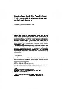
2. Problem Formulation Generally, WT is classified into two types, that is, fixed and variable speed WT. Variable speed WT has more advanced and flexible operation than fixed speed WT. Operating regions in variable speed WT are divided into three types. Figure 1 shows the various operating region in variable speed WT. Region 1 represents the wind speed below the cut-in wind speed. Region 2 represents the wind speed between cut-in and cut-out. In this region, the main objective is to maximize the energy capture from the wind with reduced oscillation on the drive train. Region 3 describes the wind speed above the cutout speed. In this region, pitch controller is used to maintain the WT at its rated power. Figure 2 shows the WT control scheme. To achieve the above objective (Region 2), the blade pitch angle (𝛽opt ) and tip speed ratio (𝜆 opt ) are set to be its optimal value. In order to achieve the optimal tip speed ratio, the rotor speed must be adjusted to the reference/optimal rotor speed (𝜔𝑟opt ) by adjusting the control input, that is, generator torque (𝑇𝑔 ). Equation (1) defines the reference/optimal rotor speed: 𝜔𝑟opt = 𝜔ref =
𝜆 opt 𝜐 𝑅
.
(1)
Prated
Aerodynamic power
Power
a Takagi-Sugeno-Kang (TSK) fuzzy model which is based on data driven model [7]. In TSK model, a combination of fuzzy clustering method and genetic algorithm (GA) is used for portioning the input-output space and least square (LS) algorithm is used for parameter estimation. Nonlinear static and dynamic state feedback linearization control are addressed in [8, 9], where both the single and two-mass model are taken into consideration and the wind speed is estimated by Newton Rapshon (NR) method. To accommodate the parameter uncertainty and robustness, a higher order sliding mode controller is proposed in [10], which ensures the stability of the controller in both regions, that is, below and above rated speed. Feedback torque control is applied for mathematical model FSWT for maximum power extraction [11]. In order to achieve the maximum power point in the WT, FLC tuned by GA is discussed in [12]. The width of the membership function in FLC is adjusted by GA. In [13], sliding mode controller (SMC) and integral sliding mode controller (ISMC) are designed for all the regions of variable speed variable pitch wind turbine (VSVPWT) with FAST simulator. The objective of this paper is to prove the efficacy of nonlinear controllers which considers the dynamic aspect of the wind and aero turbine, without the wind speed measurement. Finally, the objective is to track the reference rotor speed asymptotically. This paper is organized as follows. The objective of the work is discussed in Section 2. Section 3 discusses the modeling of the two-mass model. The conventional and proposed controllers are discussed in Sections 4 and 5. In Section 6, FAST model results are analyzed. Finally, a conclusion is drawn from the obtained results in Section 7, which shows the proposed method is having better performance compared to other existing controllers.
Wcut-out Wcut-in Region 1 Region 2
Wrated
Wind speed Region 3
Figure 1: Power operating region of wind turbines.
𝜔ropt +
−
Aero turbine control
Aero turbine
𝜔r
Figure 2: WT control scheme.
3. WT Model A WT is a device which converts the kinetic energy of the wind into electric energy. Simulation complexity of the WT purely depends on the type of control objectives. In case of WT modelling complex simulators are required to verify the dynamic response of multiple components and aerodynamic loading. Generally, dynamic loads and interaction of large components are verified by the aeroelastic simulator. For designing a WT controller, instead of going with complex simulator, the design objective can be achieved by using simplified mathematical model. In this work, WT model is described by the set of nonlinear ordinary differential equations with limited degree of freedom. In this paper, the control law is designed based on simplified mathematical model with the objective of optimal power capture at below rated wind speed and reduced oscillation of the drive train. The proposed controllers are tested with different wind profiles. Finally, the controllers are validated for FAST WT model. The parameters of the two-mass model are given in [9]. Generally, VSWT system consists of the following components; that is, aerodynamics, drive trains, and generator are shown in Figure 3. Equation (2) gives the nonlinear expression for aerodynamic power capture by the rotor: 1 𝑃𝑎 = 𝜌𝜋𝑅2 𝐶𝑃 (𝜆, 𝛽) 𝜐3 . 2
(2)
From (2), it is clear that the aerodynamic power (𝑃𝑎 ) is directly proportional to the cube of the wind speed. The power coefficient 𝐶𝑃 is the function of blade pitch angle (𝛽)
Journal of Renewable Energy
3 Tg
Ta 𝜐
Wind speed
Rotor aerodynamics
𝜔r
Drive trains
Pe
Generator
𝜔g
Figure 3: Schematic of WT.
and tip speed ratio (𝜆). The tip speed ratio is defined as ratio between linear tip speed and wind speed: 𝜔𝑅 𝜆= 𝑟 . 𝜐
(3)
Table 1: Coefficients’ values. 𝑎0 = 0.1667 𝑎1 = −0.2558 𝑎2 = 0.115
𝑃𝑎 = 𝑇𝑎 𝜔𝑟 ,
(4)
1 𝑇𝑎 = 𝜌𝜋𝑅3 𝐶𝑞 (𝜆, 𝛽) 𝜐2 , 2
(5)
where 𝐶𝑞 is the torque coefficient given as 𝐶𝑞 (𝜆, 𝛽) =
CP
Generally, wind speed is stochastic nature with respect to time. Because of this, tip speed ratio gets affected, which leads to variation in power coefficient. The relationship between aerodynamic torque (𝑇𝑎 ) and the aerodynamic power is given in (4):
0.45 0.4 0.35 0.3 0.25 0.2 0.15 0.1 0.05 0
0
𝑎3 = −0.01617 𝑎4 = 0.00095 𝑎5 = −2.05 × 10⁻⁵
2
4
6
8
10
12
14
𝜆
𝐶𝑃 (𝜆, 𝛽) . 𝜆
Figure 4: 𝐶𝑃 versus 𝜆 curve.
(6)
Substituting (6) in (5), we get Gearbox ratio is defined as
𝐶 (𝜆, 𝛽) 2 1 𝑇𝑎 = 𝜌𝜋𝑅3 𝑃 𝜐. 2 𝜆
(7)
In the above equation, the nonlinear term is 𝐶𝑃 which can be approximated by the 5th-order polynomial given in the following:
𝑛𝑔 =
𝜔𝑔 𝑇ls = , 𝑇hs 𝜔ls
(12)
𝑇ls = 𝑛𝑔 𝑇hs .
(13)
From (11), the high speed shaft torque 𝑇hs can be expressed as
5
𝑇hs = 𝐽𝑔 𝜔̇ 𝑔 + 𝐾𝑔 𝜔𝑔 + 𝑇em .
𝐶𝑃 (𝜆) = ∑ 𝑎𝑛 𝜆𝑛
(8)
𝑛=0
2
3
4
5
Putting the values of 𝑇hs from (14) in (13), we get
= 𝑎0 + 𝜆𝑎1 + 𝜆 𝑎2 + 𝜆 𝑎3 + 𝜆 𝑎4 + 𝜆 𝑎5 ,
𝑇ls = 𝑛𝑔 (𝐽𝑔 𝜔̇ 𝑔 + 𝐾𝑔 𝜔𝑔 + 𝑇em ) .
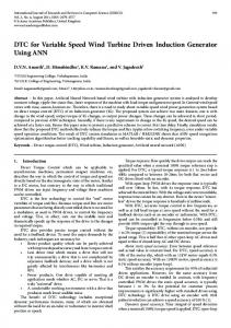
where 𝑎0 to 𝑎5 are the WT power coefficients. The values of approximated coefficients are given in Table 1. Figure 4 shows the 𝐶𝑃 versus 𝜆 curve. Figure 5 shows the two-mass model of the WT. Equation (9) represents dynamics of the rotor speed 𝜔𝑟 with rotor inertia 𝐽𝑟 driven by the aerodynamic torque (𝑇𝑎 ): 𝐽𝑟 𝜔̇ 𝑟 = 𝑇𝑎 − 𝑇ls − 𝐾𝑟 𝜔𝑟 .
(9)
Breaking torque acting on the rotor is low speed shaft torque (𝑇ls ) which can be derived by using stiffness and damping factor of the low speed shaft given in the following: 𝑇ls = 𝐵ls (𝜃𝑟 − 𝜃ls ) + 𝐾ls (𝜔𝑟 − 𝜔ls ) .
(10)
Equation (11) represents dynamics of the generator speed 𝜔𝑔 with generator inertia 𝐽𝑔 driven by the high speed shaft torque (𝑇hs ) and braking electromagnetic torque (𝑇em ): 𝐽𝑔 𝜔̇ 𝑔 = 𝑇hs − 𝐾𝑔 𝜔𝑔 − 𝑇em .
(11)
(14)
(15)
4. Conventional Controllers In order to compare the results of proposed and existing conventional controllers, a brief description of the wellknown control techniques, that is, ISC and ATF, is discussed in this section. In ISC, it is assumed that the WT is stable around its optimal aerodynamic efficiency curve. The twomass model control signal is given in the following: 𝑇em = 𝐾opths 𝜔𝑔2 − 𝐾𝑡hs 𝜔𝑔 ,
(16)
where 𝐾opths = 0.5𝜌𝜋 𝐾𝑡hs
𝑅5 𝑛𝑔3 𝜆3opt
𝐶𝑃opt ,
𝐾 = (𝐾𝑔 + 2𝑟 ) , 𝑛𝑔
(17)
4
Journal of Renewable Energy 𝜔t
Jr Ta
Tls
Bls
𝜔g Ths
Kls
Jg
Tem
Gear box (ng )
Kg
Kr
Figure 5: Two-mass model of the aero turbine.
where 𝐾𝑡hs is the low speed shaft damping coefficient brought up to the high speed shaft. In ATF, proportional control law is used to control the WT. The rotor speed and the aerodynamic torque (𝑇𝑎 ) are estimated using Kalman filter, which is used to control the WT [14]. The control law is given in (18): 𝑇em =
𝐾 𝐾 1 ̂ ̂𝑔 − 2𝐶 (𝜔𝑔ref − 𝜔𝑔 ) , 𝑇 − ( 2𝑟 + 𝐾𝑔 ) 𝜔 𝑛𝑔 𝑎 𝑛𝑔 𝑛𝑔
̂𝑎 , 𝜔𝑔ref = 𝑛𝑔 𝑘𝑤 √𝑇 𝑘𝑤 =
1 √𝑘opt
=
2𝜆3opt √ , 𝜌𝜋𝑅5 𝐶𝑃opt
1 𝑅5 𝑘opt = 𝜌𝜋 3 𝐶𝑃opt . 2 𝜆 opt
(18)
5. Proposed Nonlinear Controllers 5.1. Terminal Sliding Mode Control (TSMC) for Optimal Power Capture. Let us consider the linear sliding surface: 𝑆 = 𝛼𝑒 + 𝑒.̇
(24)
The first-order derivative of the above equation can be obtained as 𝑆 ̇ = 𝛼𝑒 ̇ + 𝑒.̈
(19)
(25)
A nonsingular terminal sliding mode manifold [15] is first designed as (20)
(21)
The optimal value of proportional gain is found to be 𝐾𝑐 = 3 × 10⁴ . The above existing control techniques have three major drawbacks, that is, the ATF control having more steady state error, so an accurate value of 𝜔𝑔ref is needed; in ISC, the WT has to operate at its optimal efficiency curve which introduces more power loss for high varying wind speed. Both the controllers are not robust with respect to disturbances. To avoid the above drawbacks, two nonlinear controllers, that is, MNSSFE and TSMC, are proposed. 4.1. Wind Speed Estimation. The estimation of effective wind speed is related to aerodynamic torque and rotor speed provided the pitch angle is at optimal value:
̇ , 𝜎 = 𝑆 + 𝛽𝑆𝑝/𝑞
(26)
where 𝛽 > 0 is a design constant and 𝑝 and 𝑞 are the positive integer, which satisfy the following condition: 𝑝 > 𝑞 or 1
0,
𝑒 = 𝜔𝑟opt − 𝜔𝑟 .
(47)
From (45), the new input 𝑤 is defined as 𝑤 = 𝜔̇ 𝑟opt + 𝑎0 𝑒.
(48)
By substituting 𝑤 in (46), we get the final control law for the WT two-mass model: 𝑇em =
𝑇𝑎 𝐾𝑟 − 𝜔 − 𝐽 𝜔̇ − 𝐾𝑔 𝜔𝑔 𝑛𝑔 𝑛𝑔 𝑟 𝑔 𝑔 𝐽 − 𝑟 (𝜔̇ 𝑟opt + 𝑎0 𝑒) . 𝑛𝑔
(49)
6. Validation Results CARTs (Control Advanced Research Turbines) are located in the center of the national wind NREL (National Renewable Energy Laboratory), near Golden, Colorado. The CART3 is a three-bladed variable speed and variable pitch wind turbine and has a rating of 600 kW. It mainly consists of three parts, namely, the rotor, the tower, and the nacelle. The generator is connected to the grid through power electronics that can directly control generator torque [16]. The power electronics consist of three-phase PWM (Pulse Width Modulation) converters with a constant dc link voltage. The main objective of the grid side converter is to maintain the dc link voltage constant [17, 18]. 6.1. Simulation Using FAST Model. FAST was developed by the NREL; it is used for WT aeroelastic simulator. The modelling of two- and three-blade horizontal axis wind turbines (HAWT) is obtained by FAST. This FAST code can be able to predict extreme and fatigue loads. Tower and flexible blade server are modelled by “assumed mode method.” WT loads are calculated by using BEM (Blade Element Momentum) and multiple component of wind speed profile [19]. FAST code is approved by the Germanischer Lioyd (GL) WindEnergie GmbH for calculating onshore WT loads for design and certification [20]. Due to the above advantages and exact nonlinear modeling of the WT, the proposed controllers are validated by using FAST. In general,
three-blade turbines have 24 DOF (degrees of freedom) to represent the wind turbine dynamics. In this work, 3 DOF are considered for WT, that is, generator, rotor speed, and blade teeter. FAST codes are interfaced with S-function and implemented with Simulink model. FAST uses an AeroDyn file as an input for aerodynamic part. AeroDyn file contains aerodynamic analysis routine and it requires status of a WT from the dynamic analysis routine and returns the aerodynamic loads for each blade element to the dynamic routine [21]. Wind profile acts as the input file for AeroDyn. The wind input file is generated by using TurbSim which is developed by the NREL. The test wind profile with full field turbulence is generated by using TurbSim developed by NREL. Figure 6 shows the hub height wind speed profile. In general, any wind speed consists of two components, that is, mean wind speed and turbulence component. The test wind speed consists of 10 min dataset that was generated using Class A Kaimal turbulence spectra. It has the mean value of 7 m/s at the hub height, turbulence intensity of 25%, and normal IEC (International Electrotechnical Commission) turbulence type. The above wind speed is used as the excitation of WT. The proposed and conventional controllers are implemented using FAST interface with MATLAB Simulink. The main objectives of the controllers are to maximize the energy capture with reduced stress on the drive train. The efficiency of the controllers is compared by using the following terms, that is, aerodynamic (𝜂aero ) and electrical (𝜂elec ) efficiency given in the following: 𝑡
𝜂aero (%) =
∫𝑡 fin 𝑃𝑎 𝑑𝑡 𝑡
ini
∫𝑡 fin 𝑃𝑎opt 𝑑𝑡
,
ini
(50)
𝑡
𝜂elec (%) =
∫𝑡 fin 𝑃𝑒 𝑑𝑡 ini
𝑡fin
∫𝑡 𝑃𝑎opt 𝑑𝑡
,
ini
where 𝑃𝑎opt = 0.5𝜌𝜋𝑅2 𝐶𝑃opt is the optimal aerodynamic power for the wind speed profile. The following objectives are used to measure the performance of the controllers: (1) Maximization of the power capture is evaluated by the aerodynamic and electrical efficiency which is defined in (50). (2) The reduced oscillation on the drive train and control torque smoothness are measured by the STD (standard deviation) and maximum value. The abovementioned values for all the controllers are given in Table 2. The rotor speed comparisons for FAST simulator are shown in Figures 7 and 8. The conventional controllers such as ATF and ISC are not able to track the optimal reference speed. ATF has only single tuning parameter, that is, 𝐾𝑐 , which allows reducing the steady state error. In ISC, during fast transient wind speed, it introduces more power loss. Moreover, these controllers are not robust with respect to high turbulence wind speed profile. To overcome the above drawbacks, TSMC and MNSSFE are proposed.
Journal of Renewable Energy
7
Control strategy STD (𝑇ls ) (kNm) Max (𝑇ls ) (kNm) STD (𝑇em ) (kNm) Max (𝑇em ) (kNm) 𝜂elec (%) 𝜂aero (%)
ISC 9.629 45.62 0.142 1.010 69.73 85.59
ATF 23.03 130.8 0.369 2.500 72.87 85.06
MNSSFE 23.13 136.7 0.280 1.807 76.23 94.67
TSMC 16.00 107.81 0.246 1.835 74.81 94.36
Rotor speed (rad/s)
Table 2: Comparison of different control strategies based on twomass model using FAST simulator.
4 3.8 3.6 3.4 3.2 3 2.8 2.6 2.4 2.2 2
0
200
300 Time (s)
400
500
600
𝜔ref ISC ATF
11 10
Figure 7: Rotor speed comparison for ATF and ISC for FAST simulator.
9 8 7 6 5 4
0
100
200
300 Time (s)
400
500
600
Figure 6: Test wind speed profile.
Figure 8 shows the rotor speed comparisons for MNSSFE and TSMC. From this figure, it is clear that at initial wind condition 0–30 sec both the controllers are not able to track the optimal rotor speed due to the initial setting in the AeroDyn input file. At high wind speed variations 220, 350, and 550 sec, the TSMC is almost tracking the reference rotor speed compared to MNSSFE. Except MNSSFE and TSMC, all the other controllers are having more tracking error in rotor speed. To achieve more power capture, the rotor speed should closely track the optimal rotor speed. Table 2 gives the performance analysis of all the conventional and proposed controllers. From Table 2, it is clear that the STD of 𝑇em and 𝑇ls is the lowest for TSMC and the highest for ATF controller. This ensures that the smoothness of the control input in TSMC is better compared to other controllers. ISC has very less STD of 𝑇em and 𝑇ls ; at the same time, the efficiency is very low compared to all the controllers. Also the ISC control only depends on the generator speed which is not accurate and for higher variation in wind speed and introduces significant power loss. So a trade-off should be made between the efficiency and the fatigue load on drive train. Except TSMC, ATF and MNSSFE are having more standard deviation which ensures more drive train transient load. Compared to ISC and ATF, the aerodynamic and electrical efficiency of the proposed TSMC and MNSSFE are better. To analyze the controller performances in a more detailed fashion, Figures 9 and 10 show the box plot for low speed shaft torque and generator torque with the mean, median, ±25% quartiles (notch boundaries), ±75% quartiles (box ends), ±95% bounds, and the outliers. From the size of the boxes
Rotor speed (rad/s)
Wind speed (m/s)
100
4 3.8 3.6 3.4 3.2 3 2.8 2.6 2.4 2.2 2
0
100
200
300 Time (s)
400
500
600
𝜔ref MNSSFE TSMC
Figure 8: Rotor speed comparison for TSMC and MNSSFE for FAST simulator.
shown, it is clear that the ISC experiences minimum variation compared to others. It ensures that ISC has the minimum transient load on the drive train; at the same time, we can find from Table 2 that the efficiency of ISC is not comparable with other controllers. Comparing the box plot of TSMC and MNSSFE, with TSMC having less variation in low speed shaft torque and generator torque, this indicates smoothness of the controller and reduction in transient load. Figure 11 shows the box plot for rotor speed for FAST simulator. From this figure, it is clear that TSMC has almost the same variation as the variation in the reference rotor speed. It is observed that, apart from TSMC and MNSSFE, other controllers such as ATF and ISC are having more variations with respect to reference speed. This indicates that, for ATF and ISC, the obtained rotor speed is not able to track the reference rotor speed. The frequency analysis is carried out by using the PSD on the low speed shaft torque which is shown in Figure 12. As the MNSSFE plot is completely above the TSMC plot, it is clear that low speed shaft torque variation is more
8
Journal of Renewable Energy Comparison of generated average powers Above baseline (%)
Low speed shaft torque (Nm)
×105
2.5 2 1.5 1 0.5 0
10
5
0 ATF
MNSSFE
SMC
−0.5 ISC
ATF MNSSFE Control strategy
Figure 13: Comparison for baseline control with other controllers for generated average power.
TSMC
Generator torque (Nm)
Figure 9: Box plot for low speed shaft torque using FAST simulator.
3000 2000 1000 0 −1000 −2000 −3000 −4000 ISC
ATF MNSSFE Control strategy
TSMC
Rotor speed (rad/s)
Figure 10: Box plot for generator torque using FAST simulator.
3.8 3.6 3.4 3.2 3 2.8 2.6 2.4 2.2 2 𝜔ref
ISC
ATF MNSSFE Control strategy
TSMC
Figure 11: Box plot for rotor speed using FAST simulator.
Periodogram using FFT
Power/frequency (dB/Hz)
180 160 140 120 100 80 60 40
0
0.5
1 1.5 Frequency (Hz)
2
2.5 ×10⁻³
MNSSFE TSMC
Figure 12: PSD for low speed shaft torque using FAST simulator.
for MNSSFE than TSMC. This ensures that TSMC gives minimum excitation to the drive train. As shown in Figure 13, the MNSSFE controller has improved power capture by 2.53% compared to TSMC. Fast tracking introduces more variation in control input and drive train. So an intermediate tracking has to be chosen and a compromise has been made between efficiency and load mitigation. From this analysis, even though MNSSFE gives a little better efficiency than TSMC, by considering transient load on drive train and smooth control input, TSMC is found to be optimal. In order to avoid the torsional resonance mode by choosing the proper tracking dynamics, a trade-off is made between power capture optimization and reduced transient load on low speed shaft torque. A good dynamic tracking, that is, similar to WT fast dynamics, gives better power capture but it requires more turbulence in control torque. Conversely slow tracking gives smooth control action with less power capture. Therefore, a compromise should be made between the power capture and transient load reduction. The better optimal speed tracking leads to better power capture for TSMC controller. The simulations are performed with different wind speed profiles with the mean wind speed at below rated wind speed. The results are given in Tables 3 and 4. From these tables, it is observed that, with an increase in mean wind speed, the maximum value of the control input (𝑇em ) also increases. In all the cases, both TSMC and MNSSFE controllers are having almost the same efficiency but the transient load reduction is better for TSMC. As the mean wind speed increases, the standard deviation also increases for MNSSFE compared with TSMC. It is observed that when the wind speed undergoes high variation the TSMC can be able to produce better power capture with reduced transient load on the drive train. Figure 14 shows the electrical power comparison for industrial baseline controller, with MNSSFE and TSMC. From this figure, it is observed that industrial baseline controller has more oscillation compared to MNSSFE and TSMC. Both MNSSFE and TSMC are almost having the same power. From Table 5, it is found that industrial baseline has more oscillation in control torque compared with other controllers. Figure 15 shows the rotor speed comparison for MNSSFE and TSMC with constant additive disturbance of 1 kNm/𝑛𝑔 .
Journal of Renewable Energy
9
Mean wind speed (m/sec) 7 (m/sec)
Electrical efficiency (%)
𝑇ls standard deviation kNm
Max (𝑇em ) kNm
74.81
16.00
1.835
8 (m/sec)
73.51
16.83
1.683
8.5 (m/sec)
73.33
13.34
1.955
Electrical power (w)
Table 3: TSMC performance for different wind speed profiles.
Table 4: MNSSFE performance for different wind speed profiles. Electrical efficiency (%)
𝑇ls standard deviation kNm
Max (𝑇em ) kNm
7 (m/sec)
76.23
23.13
1.807
8 (m/sec)
74.85
23.35
1.995
8.5 (m/sec)
74.52
23.58
2.076
Mean wind speed (m/sec)
MNSSFE
TSMC
565.00
529.96
502.89
𝜂ele (%)
73.72
77.82
75.73
Table 6: Additive disturbance performance comparison for MNSSFE and TSMC. MNSSFE
TSMC
STD (𝑇em ) kNm
0.279
0.253
STD (𝑇ls ) kNm 𝜂ele (%)
23.06 75.68
17.97 75.72
From this figure, it is clear that both controllers are robust with respect to disturbance. With reference to Table 6, the STD is less for TSMC as compared to MNSSFE; at the same time, the efficiency of these controllers is similar.
7. Conclusion This paper deals with the problem of controlling the maximum power generation at below rated wind speed of VSWT. The objective is to design a robust controller that maximizes the energy extraction from the wind while reducing the transient loads. For the above purpose, two nonlinear controllers, that is, TSMC and MNSSFE, which have the ability to reject disturbance and accommodate parameter uncertainty, are proposed in this study. Finally, it is concluded that a tradeoff is to be maintained between the efficiency and mechanical stress on the drive train. The performances of these controllers are compared with the conventional ATF and ISC using FAST aeroelastic simulator. The proposed controllers are found to produce satisfactory results in achieving the control objectives.
200
300 Time (s)
400
500
600
Figure 14: Comparison for baseline control with other controllers for electrical power.
Rotor speed (rad/s)
Baseline
100
MNSSFE BL TSMC
Table 5: Performance comparison for MNSSFE and TSMC with industrial baseline controller.
STD (𝑇em ) Nm
×105 4.5 4 3.5 3 2.5 2 1.5 1 0.5 0 0
4 3.8 3.6 3.4 3.2 3 2.8 2.6 2.4 2.2 2
With disturbance of 1 kNm/ng
0
100
200
300 Time (s)
400
500
600
𝜔ref MNSSFE TSMC
Figure 15: Rotor speed comparison for MNSSFE and TSMC with constant additive disturbance of 1 kNm/𝑛𝑔 .
Nomenclature 𝐵ls : 𝐶𝑃 (𝜆, 𝛽): 𝐶𝑞 (𝜆, 𝛽): 𝐽𝑔 : 𝐽𝑟 : 𝐾𝑔 : 𝐾ls : 𝐾𝑟 : 𝑛𝑔 : 𝑃𝑎 : 𝑃𝑒 : 𝑅: 𝑇𝑎 : 𝑇em : 𝑇hs : 𝑇ls :
Low speed shaft stiffness (N⋅m⋅rad−1 ) Power coefficient Torque coefficient Generator inertia (kg⋅m2 ) Rotor inertia (kg⋅m2 ) Generator external damping (N⋅m⋅rad−1 ⋅s−1 ) Low speed shaft damping (N⋅m⋅rad−1 ⋅s−1 ) Rotor external damping (N⋅m⋅rad−1 ⋅s−1 ) Gearbox ratio Aerodynamic power (W) Electrical power (W) Rotor radius (m) Aerodynamic torque (N⋅m) Generator (electromagnetic) torque (N⋅m) High speed shaft torque (N⋅m) Low speed shaft torque (N⋅m).
10
Conflict of Interests The authors declare that there is no conflict of interests regarding the publication of this paper.
References [1] T. Burton, D. Sharpe, N. Jenkins, and E. Bossanyi, Wind Energy Handbook, Wiley Publications, New York, NY, USA, 2001. [2] F. D. Bianchi, F. D. Battista, and R. J. Mantz, Wind Turbine Control Systems: Principles, Modelling and Gain Scheduling Design, Springer, Buenos Aires, Argentina, 2nd edition, 2006. [3] M. Sheikhan, R. Shahnazi, and A. N. Yousefi, “An optimal fuzzy PI controller to capture the maximum power for variable-speed wind turbines,” Neural Computing and Applications, vol. 23, no. 5, pp. 1359–1368, 2013. [4] C.-M. Hong, C.-H. Chen, and C.-S. Tu, “Maximum power point tracking-based control algorithm for PMSG wind generation system without mechanical sensors,” Energy Conversion and Management, vol. 69, pp. 58–67, 2013. [5] I. Kortabarria, J. Andreu, I. M. de Alegr´ıa, J. Jim´enez, J. I. G´arate, and E. Robles, “A novel adaptative maximum power point tracking algorithm for small wind turbines,” Renewable Energy, vol. 63, pp. 785–796, 2014. [6] J. M´erida, L. T. Aguilar, and J. D´avila, “Analysis and synthesis of sliding mode control for large scale variable speed wind turbine for power optimization,” Renewable Energy, vol. 71, pp. 715–728, 2014. [7] V. Calderaro, V. Galdi, A. Piccolo, and P. Siano, “A fuzzy controller for maximum energy extraction from variable speed wind power generation systems,” Electric Power Systems Research, vol. 78, no. 6, pp. 1109–1118, 2008. [8] B. Boukhezzar, H. Siguerdidjane, and M. Maureen Hand, “Nonlinear control of variable-speed wind turbines for generator torque limiting and power optimization,” Journal of Solar Energy Engineering, vol. 128, no. 4, pp. 516–530, 2007. [9] B. Boukhezzar and H. Siguerdidjane, “Nonlinear control of a variable-speed wind turbine using a two-mass model,” IEEE Transactions on Energy Conversion, vol. 26, no. 1, pp. 149–162, 2011. [10] B. Beltran, T. Ahmed-Ali, and M. E. H. Benbouzid, “High-order sliding-mode control of variable-speed wind turbines,” IEEE Transactions on Industrial Electronics, vol. 56, no. 9, pp. 3314– 3321, 2009. [11] M. Liao, L. Dong, L. Jin, and S. Wang, “Study on rotational speed feedback torque control for wind turbine generator system,” in Proceedings of the International Conference on Energy and Environment Technology (ICEET ’09), vol. 1, pp. 853–856, Guilin, China, October 2009. [12] H. M. Amine, H. Abdelaziz, and E. Najib, “Wind turbine maximum power point tracking using FLC tuned with GA,” Energy Procedia, vol. 62, pp. 364–373, 2014. [13] S. Rajendran and D. Jena, “Control of variable speed variable pitch wind turbine at above and below rated wind speed,” Journal of Wind Energy, vol. 2014, Article ID 709128, 14 pages, 2014. [14] H. Vihriala, R. Perela, P. Makila, and L. Soderlund, “A gearless wind power drive: part 2: performance of control system,” in Proceedings of the Wind Energy for the New Millennium European Conference (EWCE ’01), pp. 1090–1093, Copenhagen, Denmark, July 2001.
Journal of Renewable Energy [15] S. Mondal and C. Mahanta, “Adaptive second order terminal sliding mode controller for robotic manipulators,” Journal of the Franklin Institute, vol. 351, no. 4, pp. 2356–2377, 2014. [16] L. J. Fingersh and K. Johnson, “Controls advanced research turbine (CART) commissioning and baseline data collection,” Tech. Rep., National Renewable Energy Laboratory (NREL), 2002. [17] R. Ottersten, On control of back-to-back converters and sensorless induction machine drives [Ph.D. thesis], Chalmers University of Technology, Gothenburg, Sweden, 2003. [18] R. Pe˜na, R. Cardenas, R. Blasco, G. Asher, and J. Clare, “A cage induction generator using back to back PWM converters for variable speed grid connected wind energy system,” in Proceedings of the 27th Annual Conference of the IEEE Industrial Electronics Society (IECON ’01), vol. 2, pp. 1376–1381, IEEE, Denver, Colo, USA, December 2001. [19] M. O. L. Hansen, J. N. Sørensen, S. Voutsinas, N. Sørensen, and H. A. Madsen, “State of the art in wind turbine aerodynamics and aero elasticity,” Progress in Aerospace Sciences, vol. 42, no. 4, pp. 285–330, 2006. [20] A. Manjock, “Design codes FAST and ADAMS for load calculations of onshore wind turbines,” Tech. Rep., National Renewable Energy Laboratory (NREL), Golden, Colo, USA, 2005. [21] D. J. Laino and A. C. Hansen, “User’s guide to the wind turbine aerodynamics computer software aerodyn,” Tech. Rep., National Wind Technology Center, 2003.
Journal of
Journal of
Energy
Hindawi Publishing Corporation http://www.hindawi.com
International Journal of
Rotating Machinery
Wind Energy
Volume 2014
Hindawi Publishing Corporation http://www.hindawi.com
The Scientific World Journal Volume 2014
Hindawi Publishing Corporation http://www.hindawi.com
Volume 2014
Journal of
Structures Hindawi Publishing Corporation http://www.hindawi.com
Volume 2014
Journal of
Volume 2014
Journal of
Industrial Engineering
Hindawi Publishing Corporation http://www.hindawi.com
Hindawi Publishing Corporation http://www.hindawi.com
Petroleum Engineering
Hindawi Publishing Corporation http://www.hindawi.com
Volume 2014
Volume 2014
Journal of
Solar Energy
Submit your manuscripts at http://www.hindawi.com Journal of
Fuels Hindawi Publishing Corporation http://www.hindawi.com
Engineering Journal of
Advances in
Power Electronics Hindawi Publishing Corporation http://www.hindawi.com
Hindawi Publishing Corporation http://www.hindawi.com
Volume 2014
Volume 2014
Hindawi Publishing Corporation http://www.hindawi.com
Volume 2014
International Journal of
High Energy Physics Hindawi Publishing Corporation http://www.hindawi.com
Photoenergy International Journal of
Advances in
Volume 2014
Hindawi Publishing Corporation http://www.hindawi.com
Volume 2014
Volume 2014
Journal of
Combustion Hindawi Publishing Corporation http://www.hindawi.com
Volume 2014
Journal of
Nuclear Energy
Renewable Energy
International Journal of
Advances in
Science and Technology of
Tribology
Hindawi Publishing Corporation http://www.hindawi.com
Nuclear Installations Volume 2014
Hindawi Publishing Corporation http://www.hindawi.com
Volume 2014
Hindawi Publishing Corporation http://www.hindawi.com
Volume 2014
Hindawi Publishing Corporation http://www.hindawi.com
Volume 2014
Aerospace Engineering Hindawi Publishing Corporation http://www.hindawi.com
Volume 2014