Load Prediction Using Hybrid Model for Computational Grid Yongwei Wu1, Yulai Yuan2, Guangwen Yang3, Weimin Zheng4 Department of Computer Science and Technology, Tsinghua University, Beijing 100084, China 1, 3, 4
{wuyw, ygw, zwm-dcs}@tsinghua.edu.cn 2
[email protected]
Abstract—Due to the dynamic nature of grid environments, schedule algorithms always need assistance of a long-time-ahead load prediction to make decisions on how to use grid resources efficiently. In this paper, we present and evaluate a new hybrid model, which predicts the n-step-ahead load status by using interval values. This model integrates autoregressive (AR) model with confidence interval estimations to forecast the future load of a system. Meanwhile, two filtering technologies from signal processing field are also introduced into this model to eliminate data noise and enhance prediction accuracy. The results of experiments conducted on a real grid environment demonstrate that this new model is more capable of predicting n-step-ahead load in a computational grid than previous works. The proposed hybrid model performs well on prediction advance time for up to 50 minutes, with significant less prediction errors than conventional AR model. It also achieves an interval length acceptable for task scheduler.
I. INTRODUCTION Grid computing [1] is the high-performance and internet-based infrastructure that aggregates geographically distributed and diverse resources to deliver computational power to users in a transparent way, supporting large-scale, resource-intensive and distributed applications. Task scheduling is an important factor on improving resource usage efficiency in such a dynamic distributed environment. Obviously, system load prediction can be used to forecast task run time [18] and guide scheduling strategies, thus to achieve high performance and more efficient resource usage [2] [3] [4]. In most previous works, load prediction models, such as mean-based methods, median-based methods, autoregressive (AR) models, polynomial fitting, etc., use point value to represent future load status of workstations, clusters and grids. Papers [5] [6] [10] describe such point value prediction models and their performances. Some other works, like [11], implement interval value prediction on structural model to forecast system performance in a distributed production environment. Though point value prediction strategy has been widely adapted by recent system load prediction models, this kind of strategy do have some drawbacks for highly distributed environments. Because grid tasks usually take long run time, task scheduler in a computational grid needs a comparatively long-time-ahead prediction or an n-step-ahead prediction with large step intervals. Point value can hardly cover load variability in such a long time frame (i.e., step interval), and
1-4244-1560-8/07/$25.00 © 2007 IEEE
therefore these conventional point value prediction models do not perform well on n-step-ahead load prediction for large n. The interval value prediction model proposed in [11] addresses these two problems of point value prediction and provides valuable additional information that can be used by a task scheduler. But it does not achieve a reasonable prediction interval length, which is important for the task scheduler. Furthermore, most of the previous prediction works also ignore some problems in the history load data, which significantly affects the prediction accuracy. One problem is the load measurement error, which inherently exists in all measurement methods and can be amplified by a prediction model; another problem is the load data noise introduced by the load fluctuation in a computational grid. The tendency of history data is used by some tendency-track models, like AR model or polynomial fitting, to forecast future status. But the future load tendency might be distorted or concealed in the noisy data, and therefore misleads the tendency–track models, which will consequently impair prediction accuracy. Our contribution in this paper is that we propose a new hybrid model, which can forecast far more n-step-ahead load status than previous models and methods, with comparatively less prediction errors and acceptable prediction interval length for task scheduler and other utilities. To deal with the dynamic nature of computational grids and the needs of task schedulers, we integrate AR model with confidence interval estimate in our hybrid model, where AR model is used as a basic n-step-ahead point value prediction method, and the confidence interval of future load status is estimated based on both historical and predicted point values. In order to enhance prediction accuracy, Kalman Filter [12] is used to minimize the measurement errors of history load data, and Savitzky-Golay filter functions [17] are used as the tendency revealing tool for data noise eliminating. The results of our experiments on a real computational grid environment demonstrate that this hybrid model is of an excellent capability on n-step-ahead load prediction, and it also achieves much smaller prediction mean square error than conventional AR model. Furthermore, n-step-ahead load prediction is achieved for large n in our hybrid model as well. The corresponding prediction advance time can be up to 50 minutes, with low prediction mean square error (0.04 on average) and acceptable confidence interval length (less than 20%) for the task scheduler. The rest of this paper is organized as follows. Section II introduces the related work. Section III analyses the causes of
235
8th Grid Computing Conference
measurement errors and describes an error minimize tool – Kalman filter. Section IV presents our hybrid model on load prediction, and also introduces a signal smoothing algorithm, Savitzky-Golay filter, which is used to eliminate data noise and reveal the tendency of the data more clearly. Section V describes the experiment results of our hybrid model on a real computational grid. Finally, we conclude our work and describe our future work in section VI. II. RELATED WORK Previous works [7] [10] indicate that load has such properties as self-similarity and epochal behaviour, and is strongly correlated over time, which implies that system load is consistently predictable from the past behaviour. Therefore, correctly correlating the history data with the future values is the kernel to make accurate predictions. Several load prediction strategies in the distributed environment have been proposed in the past. [14] extends the prediction by using seasonal variation and Markov model-based meta-predictor in addition to seasonal variation for 1-step-ahead prediction. [15] proposes a multi-resource prediction model that uses both autocorrelation and cross correlation to achieve higher prediction accuracy. The Network Weather Service (NWS) provides a dynamically monitoring and forecasting method to implement 1-step-ahead prediction on network and computational resources [5]. NWS uses various prediction methods, such as mean-based methods, median-based methods, and AR methods to forecast the future system status at the same time. NWS tracks the accuracy of all predictors, and selects the one exhibiting the lowest cumulative error measure at any given moment to generate a forecast. In this way, NWS automatically identifies the best forecasting technique for any given resource. In Dinda’s paper [6], the prediction power of several linear models, including AR, MA, ARMA, ARIMA, and ARFIMA are evaluated in detail. Their results show that simple, practical models such as AR are sufficient for load prediction and AR(16) models or better are recommended for CPU load prediction. In [16], several homeostatic and tendency-track 1-step-ahead prediction strategies are presented and evaluated. Homeostatic methods assume that the load of a system always remains steady in a given time frame, while tendency-track strategies are based on the assumption that the tendency of the load variability exists in the load data, and can be properly revealed by the tendency-track models. The prediction of future value is adjusted according to the magnitudes of the last load measurement and the last prediction error, and the evaluations of this technique show that it outperforms NWS for CPU load prediction. The prediction strategies mentioned above in this section are all using point value to represent the future load status. Conventional point value prediction models are often inaccurate since they can only represent one point in a range of possible behaviours. In [11], stochastic interval values are introduced in the area of system load prediction, which can
address this problem. Authors of the paper define stochastic values using intervals, and then they define the interval arithmetic formulas and implement interval value on the point value prediction model. The interval value prediction model in [11] performs more effectively than point value prediction models in production environments. III. MEASUREMENT ERROR AND ERROR MINIMIZATION Measurement error is unavoidable in every measurement method. On one hand, the monitoring sensors bring some degrees of disturbers into target system; on the other hand, some measurement methods gain performance value by estimation, for example, computing CPU availability from the average load of the system, or using the value of a time point in a period to represent the average performance of that period. Because of these, measurement would inevitably be inaccurate. Even worse, a prediction model would amplify these measurement inaccuracies in the prediction result. In this section, we ignore the errors caused by the monitoring sensors, considering that these errors are relatively small compared with those caused by the measurement methods. In this section, the measurement error reported by the Computer Science and Engineering Department at UCSD and measurement error observed by us in Bioinformatics Application Grid (BioGrid) of ChinaGrid [20] are discussed first, followed by the introduction of the solution to the problem, which use the famous Kalman filter to minimize the error observed in the BioGrid. A. Measurement methods and errors observed by UCSD In [10], three kinds of measurement methods are given and the results gathered by monitoring a collection of workstations and compute servers in the Computer Science and Engineering Department at UCSD are reported. To determine the accuracy of these three methods, they compared the measurements of these three methods with the readings generated by an independent ten-second, CPU –bound process which they refer to as the test process. The mean absolute measurement errors of these three methods observed for different hosts at UCSD vary from as small as 3.2% to as big as 41.3%, which would inevitably deteriorate the prediction accuracy. B. Measurement methods and errors observed in the BioGrid of ChinaGrid The BioGrid of ChinaGrid (see section V for details) uses a simple method to generate the average performance value of every fixed time frame. The monitor centre gathers various performance data from the nodes of the Grid every 60 seconds, and uses the point value observed at the beginning of the monitor interval to represent the average performance of this time frame. Because the tasks running on the BioGrid are time-consuming and the CPU load of each node in the BioGrid is stable in a moderate period, we assume that the load data detected by the node sensors at a certain time point can be used to represent the average load of the time frame to which this time point belongs to. We also use the test process method in [10] to determine the measurement accuracy. We set a test process to report
236
CPU load every 10 seconds, whereas the original BioGrid sensors report the monitoring information every 60 seconds. Fig. 1 details the measurement errors observed from a node of the BioGrid.
Fig. 1 CPU load measurement errors observed on one node (in Tsinghua University) of the BioGrid. Mean absolute Measurement Error is 0.069543, and Mean Square Measurement Error is 0.0145
C. Using Kalman filter to minimize measurement errors In 1960, R.E. Kalman proposed a recursive solution to the discrete-data linear filtering problem in his famous paper [12]. Kalman filter has been extensively researched and applied, particularly in the area of autonomous or assisted navigation [9]. It provides an efficient recursive method to estimate the state of a process, and minimizes mean square error. Kalman filter uses feedback control to estimate a process: firstly the filter estimates the process state at certain time and secondly obtains feedback from the measurements. Thus we can divide the equations of Kalman filter into two groups: time update equations and measurement update equations. The specific equations for time and measurement updates are presented in [12] and [9]. Our work applies Kalman filter to minimize measurement errors, and therefore enhance prediction accuracy, which is evaluated in section V. Kalman filter has two initial parameters, process noise covariance Q and measurement noise covariance R. In practice, these two parameters might vary with each time step or measurement, but we assume they are constants here. Presuming a very small process variance, we let Q = 1e – 5, and fix the measurement variance R = (0.062)2 = 0.0036. Because this is the “true” average measurement error variance we observed from the pervious load data in the BioGrid of ChinaGrid, we would expect the “best” performance in terms of balancing responsiveness and estimate variance. IV. PREDICTION Task schedule and load balance strategies can benefit a lot from accurate load prediction. Because the load variability and resource consuming situation on a computational grid are strongly correlated over time and have the properties such as self-similarity, period stability, long time load prediction
should be feasible. In this section, we introduce our hybrid model on load prediction for computational grid, which integrates AR model with confidence interval estimate. We use AR model as the basic linear model to predict an n-step-ahead load point value, and then history load data and prediction load data are used to estimate the possible load interval of an n-step-ahead future time frame. Even with Kalman filter applied to eliminate the measurement errors, the noise still exists in the load data, and the tendency of load variability is concealed in the fluctuating data noise. We need a smoothing algorithm to expose the features of load data, and provide a reasonable starting approach for parametric fitting. If the curve of load data is smoothed, the tendency of future state would be more obvious and the prediction would be more accurate. A. Smooth history load data using Savitzky-Golay filter Savitzky-Golay smoothing filter [17] is typically used to "smooth out" a noisy signal with a large frequency span. In our work, we use Savitzky-Golay smoothing filter to smooth load data in several steps of our prediction model. Savitzky-Golay filter can be regarded as a generalized moving average. The filter coefficients are derived by implementing an unweighted linear least square fit using a polynomial of a given degree. A higher degree polynomial makes it possible to achieve a high level of smoothing without attenuating data features. For frequency data, this filter is effective at preserving the high-frequency components of the signal. In our work, we set the parameters of Savitzky-Golay filter with span=101, pd (polynomial degree) = 4. B. Predict future state using AR models and interval value In [5], the performance prediction minimum mean square error and mean percentage error values for each network setting of different prediction models are summarized. Although best predictor of each performance characteristic is, in general, not obvious and varies from resource to resource, with a series evaluation in [6], AR models are recommended to predict computing resource related metric, such as CPU load. 1) Using AR models to predict a future point value The main idea behind using a linear time series model in load prediction is to treat the sequence of periodic samples of performance, , as a realization of a stochastic process that can be modelled by linear stationary models, such as AR, MA, ARMA, ARIMA, ARFIMA, etc. [6]. The coefficients of the model can be estimated by observing past data sequence. If the action of the model can cover most of the data sequence variability, its coefficients could be used to estimate future data sequence values with low mean squared error. AR model is a model used to find an estimation of a data based on previous inputs of the data. The general form of a pth-order AR(p) model is as follows:
237
p
X t = ∑ ϕi X t − i + ε t i =1
(4.1)
AR model consists of two parts: an error or noise part ε t , and an autoregressive summation
p
∑ϕ i =1
i
TABLE I N-STEP-AHEAD AR(P) MODEL PREDICTION ALGORITHM
Compute the AR coefficients
X t − i . The summation
represents a fact that current input value depends only on the previous input values. The variable p is the order of AR model. The higher the order of AR model, the more accurate a representation will be. As the order of the model approaches infinity, we get almost an exact representation of the input data; however, the computational expense on calculating the AR(p) coefficients increases with the p order. Therefore, we should balance the prediction accuracy and the computational expense. In [6], the authors collected a large number of 1 Hz benchmark load traces, which capture all the dynamics of load signal, and subjected them to a detailed statistical analysis, drew a conclusion that AR(16) models or better are recommended for host load prediction. The problem in AR(p) analysis is to derive the "best" values for φi, given a series Xt-i. The majority of methods assume that the series Xt-i is linear and stationary. By convention the series Xt-i is assumed to be zero mean, if not this is simply another term ε t in the summation of the equation (4.1). Even for relatively large values of p, with the Burg algorithm [13] that we used to compute the AR(p) coefficients ϕ i , this can be done almost instantaneously. Then the 1-step-ahead value Xt can be easily computed. However, in highly distributed computational grid environments, 1-step-ahead load forecasting can not satisfy the demands of task scheduler. The further the load prediction of a computational grid can reach, the more appropriate the task scheduler can make scheduling strategies and balance the load. So what the scheduler in these large distributed environment needs is the n-step-ahead prediction (n = 2,3,4…or even 30,40,50..), which can forecast the load variability far more ahead before it really happens. AR(p) model attempts to predict an output Xt of a system based on the previous inputs (Xt-1, Xt-2, Xt-3...) and the coefficients ( ϕ1 , ϕ 2 ,...ϕ p ). Before we use AR(p) model to implement the n-step-ahead prediction, the following two important assumptions have to be addressed: • The coefficients of AR(p) model represent the variability of the history load data Xt-1, Xt-2,…, and they are also suitable to represent the tendency of the load in a future period, and the variability of future unknown data Xt, Xt+1…, Xt+n-2, and Xt+n-1. • The prediction of the Xt+n-1 is based on the data Xt+n-2, Xt+n-3, …, Xt, Xt-1, Xt-2,…,and only data Xt-1, Xt-2,…is the true measured data; Xt, Xt+1,…, Xt+n-2 must be computed step by step before predicting the Xt+n-1, and then Xt, Xt+1,…, Xt+n-2 can be assumed as the “true” data when we predict the Xt+n-1 . Based on these two assumptions, the n-step-ahead performance point value prediction is generated using the following algorithm in Table I.
ϕ1 , ϕ 2 ,...ϕ p
based on the
true monitoring data Xt-1, Xt-2,…; for i = 1 to n use the AR coefficients ϕ1 , ϕ 2 ,...ϕ p and Xt-1+i-1, end
Xt-1+i-2,…, to compute the Xt-1+I;
2) Confidence interval value prediction AR(p) model predicts the future load status by using point value. In practice, point value is often an ideal estimate, or a value that is accurate only for a given time frame [11]. It often represents the average load in a given time frame, and can not reflect the variability of a system in this time frame. In the highly distributed systems like grids, point values can not convey enough dynamic load information for the task scheduler to make scheduling strategies. Another type of value with the form of X±Y, or X1~X2, is referred as interval value. The load of a computational grid varies over time, and the interval value can provide an estimate of this variability in a given time frame.
Fig. 2 CPU load variability of THU node cluster of the BioGrid
Unfortunately, it is difficult to cover all the data of a given time frame in an interval value. Sometimes the load can be extremely abnormal and fluctuant in a wide range, as shown in Fig. 2. If we want to use an interval value to represent all the load variability in a time frame, it would lengthen the interval and be meaningless for grid task scheduler. In [11], many large-sample-size real phenomena generate distributions which are close to normal distribution. Therefore we can use confidence interval to estimate this large sample size normal distribution of load, and for the small sample size data, t-distribution is more suitable. This approach can eliminate some abnormal behaviour of load variability, and dramatically shorten the interval length in these situations. Confidence intervals represent a means of providing a range of values in which the fluctuation value can be expected to lie. This estimated range is calculated from a given set of sample data. Here, we set the sample size to be CIwindow+N, where CIwindow (Confidence interval window) is the basic sample windows size, and N is the additional windows size, which
238
includes the n-step-ahead prediction values generated by AR(p) model. We set the confidence level to be 95% in our experiments. The confidence interval value here is described as a pair of two point values (Xlower(t), Xupper(t)), where Xlower(t) denotes the lower limit of the load prediction of time frame t, while Xupper(t) means the upper limit of the load prediction of time frame t. In practice, suddenly abnormal load fluctuation in a computational grid does not happen frequently and often lasts transitorily, which makes this phenomenon hard to be predicted. In this paper, we assume that load is stable in most of the time, and therefore the load confidence interval prediction values should also display as two smoothness curves which reflect the stability of the load. So after we compute the n-step-ahead load confidence interval, we use Savitzky-Golay filter introduced in formula 4.1 to smooth the interval data, the lower limit data and the upper limit data, to do some corrections on the original load confidence interval prediction values.
supercomputing services for bioinformatics researchers through Web interface transparently. It is part of the China Education and Research Grid Project – ChinaGrid, an important project funded by Chinese Ministry of Education. ChinaGrid aims to integrate heterogeneous mass resources distributed in the China Education and Research Network (CERNET) into a public platform for research and education in China. The BioGrid has 7 nodes distributed in 6 distant cities of China (Beijing, Shanghai, Wuhan, Ji’nan, Lanzhou, Xi’an), and each of them is a cluster with processor number from 64 to 256. Without the loss of generality, we use a set of 7 series of CPU load data of the BioGrid from the ChinaGrid Super Vision (CGSV [19]) to evaluate our hybrid model, the total sample size is 13470. These CPU load data is gathered from the front-end machines of 7 nodes in the BioGrid every 60 seconds, and the CPU load of each node(cluster) is denoted as 0% to 100%, using point value to represent the average CPU load of every time frame. All the following evaluation results are generated from this set of CPU load data.
TABLE II LOAD PREDICTION PROCESS OF HYBRID MODEL
A. The optimal parameters of the AR(p) model There is no doubt that more accurate point value prediction in our work will lead to a nicer confidence interval value forecasting. In the conclusion of [6], AR(16) model or better are appropriate for the host load prediction. We measured the accuracy of the AR n-step-ahead prediction with different n, where the result of this measurement reveals the capability of AR(p) model in the further n-step-ahead prediction. Define the mean square prediction error as (5.1) 1 t MSEpoint_value_ prediction(t) = ∑(errorpoint_value_ prediction(i)2 ) (5.1) t + 1 i =0
1. Using Kalman filter to minimize the measurement errors of the history data Xmeasure(t), generate the more accuracy data Xfilter(t). 2. Using Savitzky-Golay filter to smooth the data Xfilter(t) with the former data Xfilter(t-1), Xfilter(t-2), …., generate the data Xsmooth(t). 3. Compute the AR(p) coefficients
ϕ1 , ϕ 2 ,...ϕ p
based on
the Xsmooth(t), Xsmooth(t-1)…
TABLE III MEAN SQUARE ERROR OF AR(P) N-STEP-AHEAD POINT VALUE PREDICTION, CPU LOAD DATA FROM THE BIOGRID, TOTAL 100%
4. For the given n-step-ahead parameter N, using the Xsmooth(t), Xsmooth(t-1)… and AR(p) coefficients ϕ1 , ϕ 2 ,...ϕ p to compute the predict future value of
P 4 8 16 32 64
Xpredict(t+1), Xpredict(t+2)…Xpredict(t+n). 5. Compute the confidence interval (Xlower(t+n), Xupper(t+n)) with sample size CIwindow+N, at confidence level 95%, using the data Xfilter(t-CIwindow+1)…,Xfilter(t-2), Xfilter(t-1), Xpredict(t), Xpredict(t+1)…Xpredict(t+n).
1 step ahead 0.1621 0.0535 0.0393 0.0406 0.0501
10 step ahead 0.1658 0.0685 0.0651 0.0635 0.0583
30 step ahead 0.2372 0.1244 0.1194 0.1034 0.1052
50 step ahead 0.2523 0.1498 0.1331 0.1346 0.1234
From Table III we notice that AR(p) model performs well at p≥16 and step ahead between 1 to 10, where the mean square error could be smaller than 0.065. The results suggest that AR(p) model can not predict much further future CPU load of the node in a computational grid. Considering the prediction accuracy and computational expense, we use p=32 in our evaluations below.
6.Using Savitzky-Golay filter to smooth the prediction interval value (Xlower(t+n), Xupper(t+n)) with the former data (Xlower(t+n-1), Xupper(t+n-1)), (Xlower(t+n-2), Xupper(t+n-2)),…, generate the smoothed prediction interval value(Xsmoothed_lower(t+n), Xsmoothed_upper(t+n)) 3) The whole prediction process The whole process of our hybrid model on n-step-ahead load prediction is described in Table II. V.EVALUATION We evaluated our hybrid model in an real grid environment, BioGrid. This computational grid provides bioinformatics
B. The accuracy of the confidence interval value prediction using hybrid model Unlike the point value prediction using AR(p) model which estimates a possible point value of a future time point, confidence interval value prediction gives a view of possible values in a future time frame. If the true CPU load measured by the monitoring system in a future time frame falls in the predicted confidence interval value, we define the prediction accuracy of this situation as 100%, in other words, the
239
prediction error is 0. The mean square error of the confidence interval value prediction is defined as (5.2), and Fig. 3 shows the evaluation results. 1 t MSE (t ) = (error (i ) 2 ) (5.2) int erval _ value _ prediction
∑
t + 1 i =0
int erval _ value _ prediction
The errorint erval _ value _ prediction (i ) here is slightly different from the error in the point value prediction. We compute the errorint erval _ value _ prediction (i) using the definition of (5.3). if
X lower (i)