they are orthogonal with respect to the weight functions, then many ... shape, but fairing into a square base, the zero contour being the boundary opposite.
Invited Paper Orthogonal Global/Local Approximation in N-dimensions: Applications to Input-Output Approximation J.L. Junkinsa , P. Singlab , D.T. Griffithb and T. Hendersonc Department of Aerospace Engineering, Texas A&M University, USA a Distinguished Professor, holder of George J. Eppright Chair b Doctoral Graduate Research Assistant c Masters Graduate Research Assistant
Abstract Several approximation ideas are presented. The main idea discussed is a weighting function technique that generates a global family of overlapping preliminary approximations whose centroids of validity lie on at the vertices of an N-dimensional grid, with vertices separated by a uniform step h. These preliminary approximations are constructed so they represent the behavior in hypercubes with a volume (2h)N centered on a typical vertex in the grid. These volumes, where the preliminary approximations are valid, overlap by 50% and are averaged in the overlapped hN volume hypercubes, interior to each contiguous set of 2N vertices, to determine final approximations. We establish an averaging method that ensures these final approximations are globally piecewise continuous with adjacent approximations determined in an analogous averaging process, to some prescribed order of partial differentiation. The continuity conditions are enforced by using a unique set of weighting functions in the averaging process. The weight functions are designed to guarantee the global continuity conditions while retaining near complete freedom on the selection of the generating local approximations. However, if the preliminary local approximations are chosen as linear combinations of a set of basis functions constructed such that they are orthogonal with respect to the weight functions, then many advantages are realized, as demonstrated in the paper. Construction of the new set of orthogonal polynomials, and several properties of these functions are novel results presented in this paper. This paper enables a first: piecewise continuous least square approximation in N-dimensions, using orthogonal functions. Several applications are given which provide a basis for optimism on the practical value of the ideas presented.
Introduction To motivate this paper, consider Figure 1. Here we have 64, 000 noisy measurements of a irregular function F(x, y). These happen to be stereo ray intersection measurements from correlation of stereo images of topography near Ft. Sill, Oklahoma; however, they could be measurements of any complicated, irregular function for which
a single global algebraic expression would likely be intractable. Suppose that it is desired to obtain a smooth, least square approximation of this function, perhaps with additional constraints imposed (e.g., in this case, the stereo correlation measurement process fails reliably over water, so the large spurious noise spikes over lakes Latonka and Elmer Thomas could be replaced by a constraint that the lake surface be at a known elevation). In lieu of a single global and necessarily complicated function, it is desired to represent the function using a family of simpler local approximations. Such local approximations would be much more attractive basis for local analysis. Alternatively, you may think of the local approximations as local Taylor series approximations (evaluated about local expansion points on a grid), or as any local approximations obtained from local measurements. However, if the local approximations are introduced without taking particular care, they will virtually certainly disagree in the value estimated for F(x, y) and the derivatives thereof at any arbitrary point, although the discrepancies may be small. In other words, global continuity is not assured, unless we introduce methodology to guarantee the desired continuity properties. These challenges are compounded in higher dimensions, if usual approximation approaches are used. It is desired to determine a piecewise continuous global family of local least squares approximations, while having freedom to vary the nature (e.g., degrees of freedom) of the local approximations to reflect possibly large variations in the roughness of F(x, y). While we are introducing the ideas in the setting of a data-fitting problem in a two dimensional space, the results are shown to be of much broader utility, and to generalize fully to approximation in an N dimensional space.
Figure 1: Approximation of irregular functions in two dimensions
From [1], we summarize some features of the weighting function approach to approx-
Figure 2: Qualitative representation of the averaging process in two dimensions
imation in two dimensions in Figure 2. From this figure, we introduce several qualitative observations: Notice the attractive properties of the weight functions: At any of the four vertices, we see the weight function (associated with the function whose centroid of validity is a given vertex) is unity, while the other three weight functions are zero at that vertex. Notice further that the weight functions have a qualitative bell shape, but fairing into a square base, the zero contour being the boundary opposite (e.g., 2-3-4) to the vertex (e.g., point 1) where the weight has a unit value. The four overlapping weight functions are a partition of unity, they add to unity everywhere in the overlapping unit region (which must be the case for an unbiased approximation). Furthermore, notice that along any boundary, only the two weight functions associated with the two approximations centered at the end points of that boundary are non-zero along that boundary, while the other two weight functions are zero (the partial derivatives of the other two weight functions are also along this boundaries). These continuity arguments on the averaged approximation of the function can be extended readily to corresponding properties on their partial derivatives: The averaged approximation osculate in value and partial derivatives with the four preliminary approximations at their corresponding vertices, and the function and both partial derivatives along any boundary are a weighted average of the corresponding two functions associated with the end point of that boundary and their partial derivatives are likewise an average of the partial derivatives of the functions at the end point of that boundary. Collectively, these observations lead to rigorous piecewise continuity of the averaged approximations, while leaving the user free to choose any preliminary local approximations desired or needed. These qualitative observations will be developed systematically in the subsequent sections and extended rigorously to approximation with arbitrary order continuity in an N dimensional space.
Approximation in 1-2- and N- dimensions using weighting functions The essential ideas can be introduced in a one-dimensional piecewise approximation problem. With reference © to Figure 3, we discussªthe one-dimensional problem. An arbitrary set of knots 1 X 2 X · · · K X · · · (vertices) are introduced at a uniform distance h apart; obviously, a non-dimensionalization of x is introduced as a ∆ local coordinate −1 ≤ I x = (X − I X)/h ≤ 1; centered on the I th vertix X = I X. The weighted average approximation is introduced as F¯I (X) = w(I x)FI (X) + w(I+1 x)FI+1 (X), for 0 ≤I x < 1
(1)
where the weighting functions w(x) used to average (blend) the two adjacent preliminary local approximations {FI (X), FI+1 (X)} are as yet un-specified. We prefer that the preliminary approximations {F1 (X), F2 (X), · · · , FK (X), · · ·} be left completely arbitrary, so long as they are smooth and represent the local behavior of F(X) well. As developed in [1], the weight function can be selected to guarantee that the averaged ¯ approximation F(X) osculates with FI (X) in value and first derivative as X → I X, ¯ and likewise F(X) osculates with FI+1 (X) in value and first derivative as X → I+1 X.
Notice that the shifted weight functions add to unity, as they must for an unbiased estimate, e.g., w(I x)+w(I x−1) = 1, or w(I x−1) = 1−w(I x) Observe that I+1 x = I x−1, so 0 ≤ I x ≤ 1, − 1 ≤ I+1 x = I x − 1 ≤ 0. Notice also the first derivative of the average of (1) at an arbitrary point is d F¯I (X) dFI (X) dFI+1 (X) dw(I x) dw(I+1 x) = w(I x) + w(I+1 x) + FI (X) + FI+1 (X) dx dx dx dx dx (2) Thus the required weight function satisfies the following boundary conditions: ( ( w(0) = w(1) = ¯ 1 ¯ 0 , at x = 1 : (3) at x = 0 : dw(x) ¯ dw(x) ¯ =0 =0 dx ¯ dx ¯ x=0
x=1
With these boundary conditions, the first term of (1) reduces to FI (X) as I x → 0 and likewise, only the first term of (2) contributes as I x → 0. Analogous arguments hold at the right end of the interval. If polynomials of lowest degree are used to satisfy the boundary conditions of (3), then the weight function can be shown [1] to be simply: ¾ ½ 1 − x2 (3 + 2x), − 1 ≤ x < 0 = 1 − x2 (3 − 2|x|) (4) w(x) = 1 − x2 (3 − 2x), 0 ≤ x ≤ 1 These are the functions plotted in Figure 3.
In the event that discrete measurements of F(X) are available, the preliminary approximations {F1 (X), © F2 (X), · · · , FK (X), · · ·} areªfit to data subsets in the ∆X = ±h regions centered on 1 X 2 X · · · K X · · · . It is evident that the final approximation on each interval is the average of overlapping weighted least square approximations, fit to shifted data lying within ±h of the vertices. For equally precise measurements of F(X), the least square process should use the same weight functions of (3). If the measurements are made with unequal expected precision, then the statistically justified weights should be scaled using the weights of (4). Note the qualitative justification: “If one least square fit is good, the average of two should be better.” Observe that simply through choosing the judicious weight functions of (4) we are guaranteed global piecewise continuity for all possible continuous local approximations {F1 (X), F2 (X), · · · , FK (X), · · ·}. One retains the freedom to vary the degree of the local approximations, as needed, to fit the local behavior of F(X), and rely upon the weight functions to enforce continuity. The generalization to 2-Dimensions is amazingly straightforward. Note that the local approximations {F11 (X1 , X2 ), F12 (X1 , X2 ), · · · , FI1 I2 (X1 , X2 ), · · ·} are valid over (2h) × (2h) regions centered on the vertices {( 1 X1 , 1 X2 ), ( 1 X1 , 2 X2 ), · · · , ( I1 X1 , I2 X2 ), · · ·}. Given four contiguous vertices: ( I1 X1 , I2 +1 X2 = ( I1 X1 , I2 X2 )
I2 X + h) 2
( I1 +1 X1 = ( I1 +1 X1 =
I1 X + h, 1 I1 X + h, 1
I2 +1 X 2 I2 X ) 2
=
I2 X + h) 2
(5)
The corresponding four preliminary approximations are valid in the (2h) × (2h) re-
Figure 3: Weighting function approximation of a 1-dimensional function
gions centered at the contiguous four nodes are denoted: FI1 ,I2 +1 (X1 , X2 ) FI1 +1,I2 +1 (X1 , X2 ) FI1 ,I2 (X1 , X2 ) FI1 +1,I2 (X1 , X2 )
(6)
The final averaged approximation valid within the h × h region bounded by the four vertices of (5) is given by 1
F¯I1 ,I2 (X1 , X2 ) =
1
∑ ∑ wi1 ,i2 ( I1 +i1 x1 , I2 +i2 x2 )FI1 +i1 ,I2 +i2 (X1 , X2 )
(7)
i1 =0 i2 =0
where, it can be verified that choosing the weight functions as wi1 ,i2 ( I1 +i1 x1 , I2 +i2 x2 ) = w( I1 +i1 x1 )w( I2 +i2 x2 )
(8)
then these functions are a partition of unity so that they satisfy 1
1
∑ ∑ wi1 i2 ( I1 +i1 x1 ,I2 +i2 xN ) = 1
(9)
i1 =0 i2 =0
as necessary for (7) to give an un-biased average. Note that if we use a common origin (the lower left vertex) for all four weight functions, then the one centered on
Figure 4: Weighting function w0,0 (x1 , x2 ) for 2-dimensional approximation
the origin is: w0,0 (x1 , x2 ) = [1 − x12 (3 ∓ 2x1 )][1 − x22 (3 ∓ 2x2 )] ≡ [1 − x12 (3 − 2|x1 |)][1 − x22 (3 − 2|x2 |)], the minus (plus) sign is for xi > 0 (xi < 0).
(10)
The remaining three weight functions are simply obtained by translating this function to the other three vertices as: w1,0 (x1 , x2 ) = w0,0 (x1 − 1, x2 ) w0,1 (x1 , x2 ) = w0,0 (x1 , x2 − 1) w1,1 (x1 , x2 ) = w0,0 (x1 − 1, x2 − 1)
(11)
These four overlapping weight functions are shown in Figure 5. The central unit square of Figure 5 is the focus of this figure, it is the region in which the final averaged approximation of (7) is valid. The process can be shifted by one unit cell in any direction and continuity arguments will lead to the conclusion that the adjacent final averaged approximations match in value and both partial derivatives along their common boundaries. We see the weight function of Figure 2 [1, 2] is obtained to within the obvious notation changes. The reason for changing notations in the present paper is that the generalization to N-dimensions follows easily from the above pattern.
The generalization of (7) and (8) are: 1
1
1
∑ ∑ ... ∑
F¯I1 ,···,IN (X1 , · · · , XN ) =
i1 =0 i2 =0
iN =0
¡
wi1 ,···,iN (I1 +i1 x1 , · · · ,IN +iN xN )
FI1 +i1 ,···,IN +iN (X1 , · · · , XN ))
(12)
and N
wi1 ,i2 ,···,iN ( I1 +i1 x1 , · · · ,IN +iN xN ) = ∏ w( Ii +ii xi )
(13)
i=1
1
1
1
∑ ∑ · · · ∑ wi1 ,···,iN ( I1 +i1 x1 , · · · ,IN +iN xN ) = 1
i1 =0 i2 =0
(14)
iN =0
The partition of unity constraint of (14) is required for an unbiased average in (12). Further, it can be verified that the unbiased average requirement of (14) is satisfied everywhere in the hypercube where averaged final approximation F¯I1 ···,IN (X1 , · · · , XN ) of (12) is valid. The above approximation approach, and minor variations of it, has been used in a wide variety of modeling problems, including mathematical modeling of topography, the earth’s gravity field, the focal plane distortions of star cameras, modeling the x2
w0,0(x1,x2)=[1−x21(3−2|x1| )][1−x22(3−2|x2|)] w0,1 w1,0(x1,x2)=w0,0(x1−1,x2) w0,1(x1,x2)=w0,0(x1,x2−1) w (x ,x )=w (x −1,x −1) 1,1
1 2
0,0
1
w1,1
2
w0,0
x1 w1,0
Figure 5: Four contiguous, overlapping weighting functions for 2-dimensional approximation.
input/output behavior of a synthetic jet actuators, and many other problems in approximation theory, geophysics, engineering, and applied science [1, 2, 3, 4, 5, 6, 7, 8]. While it has much in common with finite element methods, notice the distinction: Whereas conventional FEM methods interpolate nodal values of some distributed quantity into the continuous domain of the finite elements, this weighting function approach instead averages overlapping local approximations in such a way that piecewise continuity is achieved, with the user free to choose the local approximations. The weight functions given above, e.g. (4), (13), guarantee first order continuity. It is easy to extend this method [2] to obtain related weight functions of higher degree that guarantee mth order osculation with the preliminary approximations and mth order continuity of partial derivatives through the common boundaries with adjacent unit hypercubes with their corresponding weighted averaged final approximations. The generalized weight functions that guarantee arbitrary order continuity are given in Table 1. Only the weight function centered at the origin is tabulated, the other 2N − 1 weight functions are obtained by simply shifting the function using the origin translations to the other 2N − 1 vertices of the hypercube, analogous to (11), e.g., using the 2N − 1 origin translations: {(0, 0, 0, . . . , 0, 0, 1), (0, 0, 0, . . . , 0, 1, 0), . . . (1, 1, 1, . . . , 1, 1, 1)}
(15)
w(x) 1 0.9 0.8 0.7 0.6 0.5
m=2 m=1 m=0
0.4 0.3 0.2 0.1 0 −1
−0.5
0
0.5
1
x
Figure 6: 1-D Weighting functions for various degrees of piecewise continuity
The weight functions for the first three orders of continuity, for one and two dimensional approximation, are shown in Figures 6 and 7, respectively.
Figure 7: 2-D Weighting functions for various degrees of piecewise continuity.
Orthogonal approximation in 1-2- and N-dimensional spaces One-dimensional case Consider the approximation of a one variable function F(X). Suppose we are using the weighting function method as illustrated in Figure 3. The preliminary approximations , while arbitrary, in particular could be chosen to minimize the least square criterion Z1 1 w(x)[F(X) − FI (X)]2 dx (16) J= 2 −1
Furthermore, we consider the case that FI (X) is a linear combination of a prescribed set of linearly independent basis functions {φ0 (x), φ1 (x), · · · , φn (x)} as n
FI (X) = ∑ ai φi (x); X = I X + hx i=0
The least square criterion, making use of (16) can be written as
(17)
order of piecewise continuity
Weight Function: N
w0,0,···.0 (x1 , x2 , · · · , xN ) = ∏ w(xi ) i=1
∆
w(x), for all x ∈ {−1 ≤ x ≤ 1}, y = |x| 0
w(x) = 1 − y
1
w(x) = 1 − y2 (3 − 2y)
2
w(x) = 1 − y3 (10 − 15y + 6y2 )
3 .. .
w(x) = 1 − y4 (35 − 84y + 70y2 − 20y3 ) .. . (
m
w(x)
= 1 − ym+1
(2m+1)!(−1)m (m!)2
m
∑
k=0
(−1)k 2m−k+1
Ã
m k
!
ym−r
)
Table 1: Weight functions for higher order continuity
J
1 = J0 − cT a + aT Ma 2
(18)
where Z1
1 1 J0 = w(x)F 2 (x)dx ≡ < F(x), F(x) > (19) 2 2 −1 ¾ ½ 1 R R1 R1 w(x)F(x)φ0 (x)dx w(x)F(x)φ1 (x)dx · · · w(x)F(x)φn (x)dx cT = −1 −1 −1 © ª < F(x), φ0 (x) > < F(x), φ1 (x) > · · · < F(x), φn (x) > ≡ (20) µ00 µ01 · · · µ0n Z1 µ01 µ11 · · · µ1n T M = . = M ; µ =< φ , φ >≡ w(x)φi (x)φ j (x)dx (21) .. .. ij i j .. .. . . . −1 µ0n µ1n · · · µnn © ªT a0 a1 · · · an a ≡ (22) Observe that minimization of Eq.(18) gives the optimum (minimum integral least square fit error) coefficients as a = M −1 c
(23)
While (23) holds for an arbitrary set of linearly independent basis functions, for the
special case that the basis functions satisfy the orthogonality condition < φi (x), φ j (x) >≡
Z1
∆
w(x)φi (x)φ j (x)dx = ki δi j , ki = µii =
−1
Z1
w(x)φ2i (x)dx,
(24)
−1
the least square solution of (23), as a consequence of the diagonal M matrix, simplifies to the simple uncoupled result: < F(x), φi (x) > , i = 1, 2, · · · , n (25) ki Thus, if we can construct basis functions orthogonal with respect to the particular weight functions of Table 1, we enjoy the usual advantages of approximation of orthogonal functions in a global/local approximation setting. We consider the special case of m = 1; the construction of the corresponding orthogonal basis functions requires the Gramm-Schmidt process. Using the methods of the Appendix, it can be verified that the basis functions given in Table 2 satisfy the orthogonality conditions of (24). Note that cn in Table 2 is determined so that φn (x) satisfies the normalization, |φn (±1)| = 1. These functions are plotted in Figure 8. ai =
degree
Basis Functions φ j (x)
0
1
1
x
2
(−2 + 15x2 )/13
3 .. .
( − 9x + 28 x3 )/19 .. .
n
φn (x) =
1 cn
"
xn −
#
n−1 j ∑ φ j (x) j=0
Table 2: 1-dimensional basis functions orthogonal with respect to the weight function (x) = 1 − x2 (3 − 2|x|)
Two-dimensional case Consider the approximation of a two variable function F(X1 , X2 ). The preliminary approximations FIJ (X1 , X2 ), while arbitrary, in particular could be chosen to minimize the least square criterion 1 J= 2
Z1 Z1
−1 −1
w(x1 , x2 )[F(X1 , X2 ) − FIJ (X1 , X2 )]2 dx1 dx2
(26)
φ (x)
1
0
0.8 0.6 0.4
φ(x)
0.2
φ (x) φ4(x)
2
φ1(x)
0 φ3(x)
−0.2 −0.4 −0.6 −0.8 −1 −1
−0.5
0 x
0.5
1
Figure 8: 1-dimensional orthogonal basis functions
Furthermore, we consider the case that FIJ (X1 , X2 ) is chosen as a linear combination of a prescribed set of linearly independent basis functions {φi j (x)}; i = 1, 2, ...n; j = 1, 2, ...n. as n
n
FIJ (X1 , X2 ) = ∑ ∑ ai j φi j (x1 , x2 ); X1 = I X1 + hx1 , X2 = J X2 + hx2
(27)
i=0 j=0
In particular, consider the multiplicative structure for the weight function w(x1 , x2 ) = [1 − x12 (3 − 2|x1 |)][1 − x22 (3 − 2|x2 |] and basis functions
φi j (x1 , x2 ) = φi (x1 )φ j (x2 )
(28) (29)
where we choose the one-dimensional basis functions φi (x) from Table 2 that are orthogonal with respect to w(x) = 1 − x2 (3 − 2|x|). Introducing the inner product notation: ∆
< α(x1 , x2 ), β(x1 , x2 ) >=
Z1 Z1
w(ξ1 , ξ2 )α(ξ1 , ξ2 )β(ξ1 , ξ2 )dξ1 dξ2
(30)
−1 −1
As a consequence of the orthogonality φi (x) from Table 2 , the choice of (28), (29) and the definition, it is evident that the functions of (28) are orthogonal, because ∆
< φi j (x1 , x2 ), φlm (x1 , x2 ) > =
Z1 Z1
−1 −1
w(ξ1 )w(ξ2 )φi j (ξ1 , ξ2 ), φlm (ξ1 , ξ2 )dξ1 dξ2
=
Z1
w(ξ1 )φi (ξ1 )φl (ξ1 )dξ1
−1
|
= ki δil k j δ jm
Z1
w(ξ2 )φ j (ξ2 )φm (ξ2 )dξ2
−1
{z
ki δil
}|
{z
}
k j δ jm
(31)
As a consequence of orthogonality, it follows that the least square amplitudes are: ai j =
< φi j (x1 , x2 ), F(X1 , X2 ) > < φi j (x1 , x2 ), F(X1 , X2 ) > = < φi j (x1 , x2 ), φi j (x1 , x2 ) > ki k j
(32)
The first five sets (degrees zero through four) of the two dimensional orthogonal polynomials of (29) are shown in Figure 9.
Figure 9: 2-dimensional orthogonal basis functions
N-dimensional case Consider the approximation of a function F(X1 , X2 , · · · , XN ) of N variables. The preliminary approximations FI1 ···IN F(X1 , X2 , · · · , XN ), while arbitrary, in particular could be chosen to minimize the least square criterion 1 J= 2
Z1 Z1
···
−1 −1
Z1
w(x1 , · · · , xN )[F(X1 , · · · , XN ) − FI1 ···IN (X1 , · · · , XN )]2 dx1 · · · dxN
−1
(33) Furthermore, we consider the case that FI1 ···IN F(X1 , X2 , · · · , XN ) is chosen as a linear combination of a prescribed set of linearly independent basis functions {φi1 ···iN (x1 , · · · , xN )} as FI1 ···IN (X1 , · · · , XN ) =
n
n
i1 =0
iN =0
∑ · · · ∑ ai1 ···iN φi1 ···iN (x1 , · · · , xN )
(34)
where, X1 =
I1
X1 + hx1 , · · · , XN =
IN
XN + hxN
(35)
In particular, consider the continued product structure for the weight function N
w(x1 , · · · , xN ) = [1 − x12 (3 − 2|x1 |)] · · · [1 − xN2 (3 − 2|xN |] = Π [1 − xi2 (3 − 2|xi |)] (36) i=0
and basis functions N
φi1 ···iN (x1 , · · · , xN ) = Π φi (xi )
(37)
i=0
where we choose the one-dimensional basis functions φi (x) from Table 2 that are orthogonal with respect to w(x) = 1 − x2 (3 − 2|x|). Introducing the inner product notation: < α(x1 , · · · , xN ), β(x1 , · · · , xN ) > ∆
=
Z1
−1
...
Z1
w(ξ1 , · · · , ξN )α(ξ1 , · · · , ξN )β(ξ1 , · · · , ξN )dξ1 · · · dξN
(38)
−1
As a consequence of the orthogonality φi (x) from Table 2 , the choice of (33), (36), and (37) it is evident that the functions of (34) are orthogonal, because < φi1 ···iN (x1 , · · · xN ), φ j1 ··· jN (x1 , · · · xN ) > =
Z1
−1
...
Z1
(w(ξ1 ) . . . w(ξN )φi1 ···iN (ξ1 , · · · , ξN )φ j1 ··· jN (ξ1 , · · · , ξN )) dξ1 · · · dξN
−1
= [ki1 ki2 · · · kiN ][δi1 j1 δi2 j2 · · · δiN jN ]
(39)
As a consequence of orthogonality, it follows that the least square amplitudes are: =
ai1 ···iN
< φi1 ···iN (x1 , · · · , xN ), F(X1 , , · · · , XN ) > N
∏ kj
j=1
Remarkably, the weight functions, basis functions, and orthogonality conditions are generated directly from the one dimensional results. Furthermore, we arrive with a piecewise continuous approximation in N dimensions with the added benefits that the local approximations are linear combinations of basis functions orthogonal to the weight function used in averaging the overlapping approximations.
Illustrative examples The approximation algorithm presented in this paper was tested on a variety of test functions and experimental data obtained by wind tunnel testing of synthetic jet actuation wing. In this section, we present some results from the studies, importantly a test case for function approximation and a dynamical System identification from wind tunnel testing of synthetic jet actuation wing. Also, a vibrating Space Based Radar (SBR) antenna surface approximation is considered. Function approximation The test case for the function approximation is constructed using by the following analytic surface function [9]. f (X1 , X2 ) = +
5 10 + (X2 − X12 )2 + (1 − X1 )2 + 1 (X2 − 8)2 + (5 − X1 )2 + 1 5 (40) 2 (X2 − 8) + (8 − X1 )2 + 1
A random sampling of the interval [0 − 10, 0 − 10] for X1 and X2 is used to obtain 60 samples of each. Figure 10(b) shows the true surface plot of the training set data points. According to our experience this particular function has many important features such as sharp ridge line that is very difficult to learn with many existing function approximation algorithms with reasonable number of nodes. To approximate the function given in equation (40), we divide the whole input region into a set of finite element cells, defined with cartesian coordinates, X1 and X2 . Therefore, 10 × 10 modeling region can be divided into different number of cells depending upon cell length. For example, the whole input region can be modeled by a total of 16 cells of dimension 1.2766 × 1.2766 or by a total of 576 cells of dimension 0.4082 × 0.4082. Further, a grid of all function observations is generated from measurement data and a continuous approximation for a particular cell is generated via a least-square procedure.
The local approximation of analytical function fˆ(x1 , x2 ), for a particular cell is modeled by orthogonal polynomials of the form: fˆ(x1 , x2 ) = ∑ ∑ ai j φi (x1 , x2 )φ j (x1 , x2 ), i + j ≤ 2 i
(41)
j
The orthogonal functions (listed in table 2), φi and φ j , are chosen in such a way that the degree of fˆ(x1 , x2 ) is always less than or equal to 2. Further, x1 and x2 denote the local cell coordinates defined as below: x1 = 2(X1 − X1m )/X1cell
x2 = 2(X2 − X2m )/X2cell
(42)
where, (X1m , X2m ) and X1cell × X2cell represent the centroid and dimension of a particular cell respectively. As φi and φ j are chosen to be orthogonal polynomial functions therefore, unknown coefficients ai j can be determined from Equation (32). For a discrete observation grid the inner product in equation (32) is replaced by following equation: < φi j (x1 , x2 ), φkl (x1 , x2 ) >=
N
∑ w(x1m , x2m )φi j (x1m , x2m )φkl (x1m , x2m )
(43)
m=1
where, N is the total number of observation points. Now, due to discrete observations the orthogonal condition of Equation (31) can break down i.e. < φi j (x1 , x2 ), φkl (x1 , x2 ) > 6= ki δik k j δ jl . However, we should mention that as N → ∞ the orthogonality error for discrete observation decreases to zero. Figure 10(a) shows the plot of discrete orthogonalization error, defined as || < φi j (x1 , x2 ), φkl (x1 , x2 ) > −ki δik k j δ jl ||, versus number of observation points in a particular cell. From this plot, it is clear that orthogonalization error decreases as number of points inside a particular cell increases. In a future paper, we will present a procedure to generate discrete orthogonal polynomials of many variables. As discussed earlier the approximation error depends upon the grid size, therefore, it was decided to study the root mean square approximation error as a function of cell size for a fixed order of polynomials. Figure 10(e) shows the plot of root mean square approximation error versus cell size. From this figure, it is apparent that root mean square error shows a minimum value for a particular cell size. It is due to the fact that approximation error depends upon cell size and total number of observations in a particular cell. To achieve better approximation accuracy, we would like to have more observations in a particular cell and simultaneously would like to reduce the size of cell to capture the local behavior of the unknown function. However, for a fixed number of total observations, the number of observations in a particular cell decreases as cell size is reduced and increases as cell size is increased. It is due to this reason, approximation error is minimum for a particular size of finite element cell. Finally, Figures 10(c) and 10(d) show surface plots of approximated surface and relative error surface respectively. These results corresponds to total 256 cells of length 0.6186. The relative percentage approximation error is computed at cell
1.6 1.4
Orthogonality Error
1.2 1 0.8 0.6 0.4 0.2 0 0
1000
2000 3000 Number of Data Points
4000
5000
(a) Orthogonalization error vs number of data points
8 1
4
6
estimated
6
4
f
f
true
1
2
2
(X ,X )
10
8 (X ,X )
10
2
2
10
10
10 5
10
5
X
2
0
X2
X1
0
8
5
6 4 0
(b) True surface
2
X1
0
(c) Approximated surface
−5
8
x 10
7 6 5 Mean Error
Approximation Error (%)
1 0.5 0
4 3
−0.5
2 10 10
1
8
5 X2
6 4 0
2 0
(d) Error surface
X1
0 0.4
0.5
0.6
0.7
0.8 0.9 Grid Size
1
1.1
(e) Approximation error vs grid size
Figure 10: Local polynomial approximation results for May-West function
1.2
1.3
centroid using following formula: Relative error =
fapprox − ftrue × 100 ftrue
(44)
From these figures, it is clear that we are able to learn the analytical function given in Equation (40) very well with relative approximation errors less than 1%. Synthetic jet actuator modeling In this section, the local polynomial approximation results for the synthetic jet actuator are presented. These results show the effectiveness of the local polynomial approximation algorithm presented in this paper to learn the input-output mapping for the synthetic jet actuation wing. Experimental set-up
A Hingeless-Control-Dedicated experimental setup has been developed, as part of the initial effort, the heart of which is a stand-alone control unit, that controls all of the wing’s and SJA’s parameters and variables. The setup is installed in the 3′ × 4′ wind tunnel of the Texas A&M Aerospace Engineering Department (Figure 11). The test wing profile for the dynamic pitch test of the synthetic jet actuator is a NACA 0015 airfoil. This shape was chosen due to the ease with which the wing could be manufactured and the available interior space for accommodating the synthetic jet actuator (SJA). Experimental evidence suggests that a SJA, mounted such that its jet exit tangentially to the surface, has minimal effect on the global wing aerodynamics at low to moderate angles of attack. The primary effect of the jet is at high angles of attack when separation is present over the upper wing surface. In this case, the increased mixing associated with the action of a synthetic jet, delays or suppresses flow separation. As such, the effect of the actuator is in the non-linear post stall domain. To learn this nonlinear nature of SJA experiments were conducted with the control-dedicated setup shown in Figure 11. The wing angle of attack (AOA) is controlled by the following reference signal. 1. Oscillation type: sinusoidal Oscillation magnitude: 12.5◦ . 2. Oscillation offset (mean AOA): 12.5◦ 3. Oscillation frequency: from 0.2 Hz to 20 Hz. In other words, the AOA of airfoil is forced to oscillate from 0◦ to 25◦ at a given frequency (see Figure 12). The experimental data collected were the time histories of the pressure distribution on the wing surface (at 32 locations). The data was also integrated to generate the time histories of the lift coefficient and the pitching moment
Figure 11: Hingeless control-dedicated experimental setup for Synthetic Jet Actuation wing
coefficient. Data was collected with the SJA on and with the SJA off (i.e. with and without active flow control). All the experimental data were taken for 5 s at a 100 Hz sampling rate. The experiments described above were performed at a freestream velocity of 25 m s−1 . From the surface pressure measurements, the lift and pitching moment coefficients were calculated via integration. As the unknown SJA model is known to be dynamic in nature so SJA wing lift force and pitching moment coefficients are modelled by second order system i.e. they are assumed to be function of current and previous time states (angle of attack). CL (tk ) = CL (αtk ,CL (tk−1 ))
(45)
CM (tk ) = CM (αtk ,CM (tk−1 ))
(46)
Like in the function approximation example, the moment and lift data is grided based upon the time interval. To approximate the dynamics in a particular time interval the orthogonal functions, φi j , listed in Table 2 are used. CL (tk ) =
∑ ∑ ai j φi (α(tk ))φ j (CL (tk−1 )), i + j ≤ 2 i
j
30
25
25
20
20 Angle of Attack (deg.)
Angle of Attack (deg.)
30
15
10
15
10
5
5
0
0
−5 0
1000
2000 3000 Sample Number
4000
(a) Angle of attack variation without SJA.
5000
−5 0
1000
2000 3000 Sample Number
4000
5000
(b) Angle of attack variation with SJA actuation frequency of 60 Hz.
Figure 12: Angle of attack variation. CM (tk ) =
∑ ∑ ai j φi (α(tk ))φ j (CM (tk−1 )), i + j ≤ 2 i
(47)
j
Figure 13(a) shows the plot of root mean square lift force approximation error versus the size of the local time interval. From this figure, it is clear that the approximation error increases as the size of the local time interval increases. We mention that if time interval size is less than 25 then we face the problem of ill-conditioned matrix as observation points are pretty close to each other. Figures 13(b) and 13(c) show the measured and approximated lift coefficient for zero and 60 Hz jet actuation frequency respectively with time interval size of 25. Figures 13(d) and 13(e) show the corresponding approximation error plots. From these figures, it is clear that we are able to learn the nonlinear relationship between lift coefficient and angle of attack with and without SJA on. Similarly, Figures 14(a) and 14(b) show the measured and RBFN approximated pitching moment coefficient for zero and 60 Hz jet actuation frequency respectively. Figures 14(c) and 14(d) show the corresponding approximation error plots. From these figures, it is clear that we are able to learn the nonlinear relationship between moment coefficient and angle of attack (with and without SJA on) very well within experimental accuracy. Space Based Radar (SBR) antenna simulation Space Based Radar systems envisioned for the future may be a constellation of spacecraft that provide persistent real-time information of ground activities through the
−4
1.5
x 10
1.3 1.2 1.1 1 0.9 0.8 0.7
Root Mean Square Approximation Error
1.4
0.6 0.5 0
50
100
150
Number of Time Steps
200
(a) Approximation error vs grid size
1.8
1.8 Experimental Data Approximated Data
1.6
1.4
1.4
1.2
1.2
0.8 0.6
0.8 0.6
0.4
0.4
0.2
0.2 0
0 −0.2 0
Experimental Data Approximated Data
1
1 Lift Force
Lift Force
1.6
1000
2000
3000
4000
−0.2 0
5000
1000
3000
4000
5000
(c) 60 Hz approximation frequency
0.2
0.5
0.15
0.4
0.1
0.3
0.05
0.2 Approximation Error
Approximation Error
(b) 0 Hz actuation frequency
0 −0.05 −0.1
0.1 0 −0.1
−0.15
−0.2
−0.2
−0.3 −0.4
−0.25 −0.3 0
2000
Sample Number
Sample Number
1000
2000
3000
4000
5000
−0.5 0
1000
2000
Sample Number
(d) Approximation error for 0 Hz actuation frequency
3000
4000
5000
Sample Number
(e) Approximation error for 60 Hz actuation frequency
Figure 13: Lift force approximation results
0.3 Experimental Data Approximated Data
0.15 Experimental Data Approximated Data
0.1
0.2
0.05 0 Pitching Moment
Pitching Moment
0.1
−0.05
0
−0.1
−0.1
−0.15 −0.2
−0.2
−0.25
−0.3 −0.3
−0.4 0
1000
2000
3000
Sample Number
4000
5000
−0.35 0
0.08
0.1
0.06
0.08
0.04
0.06
0.02
0.04
0
−0.02
3000
Sample Number
4000
5000
0.02 0
−0.02
−0.04 −0.06
−0.04
−0.08
−0.06
−0.1
−0.08
−0.12 0
2000
(b) 60 Hz approximation frequency
Approximation Error
Approximation Error
(a) 0 Hz actuation frequency
1000
1000
2000
3000
Sample Number
4000
5000
(c) Approximation error for 0 Hz actuation frequency
−0.1 0
1000
2000
3000
4000
5000
Sample Number
(d) Approximation error for 60 Hz actuation frequency
Figure 14: Pitching moment approximation results identification and tracking of moving targets, high-resolution synthetic aperture radar imaging, and collection of high-resolution terrain information. The accuracy of the information obtain from SBR systems depend upon many parameters like the geometric shape of the antenna, permittivities of the media through which radar wave is traveling, etc. Therefore the characteristics of the scattered wave received by the SBR antenna for a given frequency depend on the surface and geometric parameters of the radar. Therefore, to apply necessary corrections for scattering of radar waves the precise knowledge of SBR antenna becomes a necessity. However, excitation of flexible dynamics mode makes shape estimation problem a bit difficult. While a variety of surface models can be employed to model the instantaneous shape, we consider the case that the surface is measured at discrete points and a smooth least square model is
desired. The objective of this section is to apply the local polynomial approximation methodology, developed in this paper, to estimate the real time SBR antenna shape.
10 8 6 4 2
Z
0 −2 −4 −6 −8 0 0.5 1 Y
−10 4
2
0
X
Figure 15: Nominal SBR Antenna Shape
For simulation, purposes the SBR antenna (shown in Figure 15) is assumed to be 20 m long and have a constant cross section along the length given by the following undeformed surface shape: X=
3 cos θ0 1+1.9 sin θ0 ,
Y=
3 sin θ0 1+1.9 sin θ0 ,
0 ≤ θ0 ≤
3π 4
(48)
To construct the shape of antenna it is assumed that measurements of 25 points are available along a given cross section with the help of some vision sensor. Further, such 20 cross section measurements are assumed to be available along the length of the antenna at a particular time with a sampling frequency of 10 Hz. Further, true measurements are corrupted by Gaussian white noise of standard deviation of 1 mm. To make the shape estimation problem more interesting the shape of antenna is assumed to vary with respect to both in spatial coordinates and time according to following equations: r sin θ r cos θ X = 1+1.9 (49) sin θ , Y = 1+1.9 sin θ π cos(πZ) sin(10t). where, r = 3 + 0.4 cos(5πZ) sin(5t) and θ = θ0 + 50
Further, the expression for r and θ can be assumed to depict the bending and torsion mode for SBR antenna. However, this motion is just representative and may be a poor approximation of the actual flexible dynamics. We mention that in this paper, we do
not worry about the actual flexible dynamics of the SBR antenna, as our purpose is just to demonstrate the local approximation methodology developed in this paper. To approximate the SBR antenna shape at a particular time, the measurement data is gridded using a set of finite element cells of size 2m×2m×3m, defined with cartesian coordinates, X, Y and Z. Now, a continuous approximation, of SBR antenna shape, for a particular cell is generated via a least-square procedure as listed in section . The SBR antenna shape for a particular cell is modeled by orthogonal polynomials given in Table 2: x(x, ˆ y, z) =
∑ ∑ ∑ ai jk φi (x)φ j (y)φk (z), i + j + k ≤ 2
(50)
∑ ∑ ∑ almn φl (x)φm (y)φn (z), l + m + n ≤ 2
(51)
i
y(x, ˆ y, z) =
l
j
k
m n
(52) It should be noticed that, x, y, and z denote the local cell coordinates defined as below: x = 2(X − Xm )/Xcell
y = 2(Y −Ym )/Ycell
z = 2(Z − Zm )/Zcell
(53)
where, (Xm ,Ym , Zm ) and Xcell ×Ycell × Zcell represent the centroid and dimension of a particular cell respectively. Figure 16 shows the true and approximated shape of the SBR antenna at different time intervals. While, Figure 17 shows the contour plots for the difference between nominal and instantaneous antenna shape. From these figures, it is clear that mean RMS approximation error for X and Y coordinate are even less than half a percent at all time intervals. Therefore, we can conclude that we are able to learn the SBR antenna shape precisely even in presence of measurement errors. However, we should mention that approximation accuracy will depend upon the order of polynomials used as well as the excited flexible dynamics mode.
Concluding remarks We have presented a general methodology for input/output mapping in N dimensions. The method averages overlapping local preliminary approximations whose centroids of validity lie at the vertices of a user specified N dimensional grid. For simplicity in this paper, the grid was taken as uniform, however the grid is more generally non uniform. The averaging makes use of a special class of weight functions that guarantee a prescribed degree of piecewise continuity and osculation with the preliminary approximations at their centroids of validity. The preliminary approximations can be chosen arbitrarily to take advantage of prior knowledge of a particular problem. Alternatively, the preliminary approximations can be chosen as linear combinations of any complete set of linearly independent basis functions. A particularly attractive choice is shown to be polynomial basis functions that are orthogonal with respect to the weight functions of the averaging process. We constructed these new orthogonal
Mean RMS Error For x=0.014976% Mean RMS Error For y=0.0032949%
Mean RMS Error For x=0.0065105% Mean RMS Error For y=0.0018116%
Time, t=8
Time, t=2
True Antenna Shape
True Antenna Shape
Approximated Antenna Shape
(a) Time, t=2 s
(b) Time, t=8 s
Mean RMS Error For x=0.0093681% Mean RMS Error For y=0.0046587% Time, t=16
Approximated Antenna Shape
Mean RMS Error For x=0.0074273% Mean RMS Error For y=0.001395% Time, t=20
True Antenna Shape
Approximated Antenna Shape
(c) Time, t=16 s
True Antenna Shape
Approximated Antenna Shape
(d) Time, t=20 s
Figure 16: Space Based Radar antenna simulation results: true and approximated surface plots. polynomials using a Gramm Schmidt process. The result is an new method for orthogonal function local approximation with an associated averaging process giving a global piecewise continuous approximation. The broad generality of the method, together with a number of examples presented provides a strong basis for optimism for the importance and utility of these ideas.
Appendix Gram-Schmidt procedure of orthogonalization Let V be a finite dimensional inner product space spanned by basis vector functions {w1 , w2 , · · · , wn }. According to the Gram-Schmidt Process an orthogonal set of basis functions {v1 , v2 , · · · , vn } can be constructed from any basis functions {w1 , w2 , · · · , wn } by following three steps: 1. Initially there is no constraining condition on the first basis element v1 therefore we can choose v1 = w1 . 2. The second basis vector, orthogonal to the first one, can be constructed by
Mean RMS Error For x=0.0065105% Mean RMS Error For y=0.0018116%
8
8
8
6
6
6
6
4
4
4
4
2
2
2
2
0
0
Z
10
8
Z
10
0
0
−2
−2
−2
−2
−4
−4
−4
−4
−6
−6
−6
−6
−8
−8
−8
−8
−10 −1
−10 −1
−10 −1
−10 −1
0
1
2
3
4
X True Contours
0
1
2
3
4
0
1
4
4
2
2
2
6
4
2
0
Z
6
4
6
Z
8
6
8
0
−2
−2
−2
−4
−4
−4
−4
−6
−6
−6
−6
−8
−8
−8
0
1
2
3
X True Contours
4
−10 −1
0
2
3
4
0
−2
−10 −1
1
Mean RMS Error For x=0.0074273% Mean RMS Error For y=0.001395%
Time, t=20
10
8
0
X Approximated Contours
8
10
Z
4
10
10
0
3
(b) Time, t=8 seconds
Mean RMS Error For x=0.0093681% Mean RMS Error For y=0.0046587%
Time, t=16
2
X True Contours
X Approximated Contours
(a) Time, t=2 seconds
Z
Mean RMS Error For x=0.014976% Mean RMS Error For y=0.0032949%
Time, t=8
10
Z
Z
Time, t=2 10
1
2
3
4
X Approximated Contours
−10 −1
−8
0
1
2
3
X True Contours
(c) Time, t=16 seconds
4
−10 −1
0
1
2
3
4
X Approximated Contours
(d) Time, t=20 seconds
Figure 17: Space Based Radar Antenna Simulation Results: True and Approximated Contour Plots (y = f (X, Z,t) − f (X0 , Z0 ,t0 )). satisfying the following condition: < v2 , v1 >= 0
(54)
v2 = w2 − cv1
(55)
Further, if we write: then we can determine the following value of unknown scalar constant c by substituting this expression for v2 in orthogonality condition, given by equation
(54): c=
< w2 , v1 > < v1 , v1 >
(56)
3. Continuing the procedure listed in step 2, we can write vk as: vk = wk − c1 v1 − c2 v2 − · · · − ck−1 vk−1
(57)
where, the unknown constants c1 , c2 , · · · , ck−1 can be determined by satisfying following orthogonality conditions: < vk , v j >= 0
For j = 1, 2, · · · , k − 1
(58)
Since, v1 , v2 , · · · , vk−1 are already orthogonal to each other therefore the scalar constant c j can be written as: cj =
< wk , v j > < v j, v j >
(59)
Therefore, finally we have following general Gram-Schmidt formula for constructing the orthogonal basis vectors v1 , v2 , · · · , vn : k−1 k j v j , j=1
vk = wk − ∑
For k = 1, 2, · · · , n
(60)
To construct the orthogonal polynomials of degree ≤ n with respect to weight function, 1 − x2 (3 − 2|x|) on closed interval [−1, 1], we need to apply the Gram-Schmidt procedure to non-orthogonal monomial basis 1, x, x2 , · · · , xn . First of all, we compute the general expression for < xk , xl >: k
l
< x , x >=
Z1
xk+l (1 − x2 (3 − 2|x|))dx =
−1
½
2 k+l+1
6 4 − k+l+3 + k+l+2 0
k + l is even k + l is odd
(61) According to this formula, monomials of odd degree are orthogonal to monomials of even degree. Now, if p0 (x), p1 (x), · · · denote the resulting orthogonal polynomials then we can begin the process of Gram-Schmidt orthogonalization by letting: p0 (x) = 1
(62)
According to equation (60), the next orthogonal polynomial is p1 (x) = x −
< x, p0 > p0 (x) = x < p0 , p0 >
(63)
Further, recursively using the Gram-Schmidt formula given by Equation (60), we can generate the orthogonal polynomials given in Table 2, including the recursive form given for φn (x).
Acknowledgement The author(s) wish to acknowledge the support of the Texas Institute for Intelligent Bio-Nano Materials and Structures for Aerospace Vehicles, funded by NASA Cooperative Agreement No. NCC-1-02038. Any opinions, findings, and conclusions or recommendations expressed in this material are those of the authors and do not necessarily reflect the views of the National Aeronautics and Space Administration.
References [1] John L. Junkins, G. W. Miller, and J. R. Jancaitis. A weighting function approach to modeling of geodetic surfaces. Journal of Geophysical Research, 78(11):1794–1803, April 1973. [2] James R. Jancaitis and John L. Junkins. Modeling in n dimensions using a weighting function approach. Journal of Geophysical Research, 79(23):3361– 3366, August 1974. [3] John L. Junkins and R. S. Engels. The finite element approach in gravity modeling. Manuscripta Geodaetica, 4:185–206, February 1979. [4] John L. Junkins. An investigation of finite element representations of the geopotential. AIAA Journal, 14(6):803–808, June 1976. [5] Remi C. Engels and John L. Junkins. Local representation of the geopotential by weighting orthonormal polynomials. AIAA Journal of Guidance and Control, 3(1):55–61, Jan-Feb 1980. [6] Puneet Singla, T. D. Griffith, Kamesh Subbarao, and J. L. Junkins. Autonomous focal plane calibration by an intelligent radial basis network. AAS/AIAA Spaceflight Mechanics Conference. Mauii, Hawaii, Febrauary 2004. [7] P. Singla, K. Subbarao, O. Rediniotis, and J. L. Junkins. Intelligent multiresolution modeling: Application to synthetic jet actuation and flow control. In 42nd AIAA Aerospace Sciences Meeting and Exhibit, number AIAA-20040774, Reno, Nevada, Jan 5-8 2004. [8] T. D. Griffith, P. Singla, and J. L. Junkins. Autonomous on-orbit calibration approaches for star cameras. In AAS/AIAA Space Flight Mechanics Meeting, number 02-102, San-Antonio, TX, Jan 27-30 2002. AAS. [9] John L. Junkins and James R. Jancaitis. Smooth irregular curves. In Photogrammetric Engineering, pages 565–573, June 1972. [10] Wing Kam Liu, Shaofan Li, and Ted Belytschko. Moving least square reproducing kernel methods (i) methodology and convergence. Computer Methods in Applied Mechanics and Engineering, 143(1-2):143–157, Aug 1997.
[11] D. Levin. The approximation power of moving least squares. Mathematics of Computations, 67:1517–1531, 1998. [12] H. Wendland. Local polynomial reproduction and moving least squares approximation. IMA Journal of Numerical Analysis, 21:285–300, 2001. [13] J. L. Crassidis and J. L. Junkins. An Introduction To Optimal Estimation Of Dynamical Systems. CRC Press, March 2004. Text Book In Press.