Jan 10, 2013 - W. Nazarewicz, N. Schunck, and M. V. Stoitsov, Phys. Rev. C 78, 014318 (2008), arXiv:0805.4446. [11] R. W. Hamming, Numerical Methods for ...
int-pub-12-056
Time-Dependent Superfluid Local Density Approximation Aurel Bulgac,1 Michael McNeil Forbes,1,2 1 Department
arXiv:1301.2024v1 [cond-mat.quant-gas] 10 Jan 2013
2 Institute
of Physics, University of Washington, Seattle, WA 98195–1560, USA, and for Nuclear Theory, University of Washington, Seattle, Washington 98195–1550 USA
The time-dependent superfluid local density approximation (tdslda) is an extension of the Hohenberg-Kohn density functional theory (dft) to time-dependent phenomena in superfluid fermionic systems. Unlike linear response theory, which is only valid for weak external fields, the tdslda approach allows one to study non-linear excitations in fermionic superfluids, including large amplitude collective modes, and the response to strong external probes. Even in the case of weak external fields, the tdslda approach is technically easier to implement. We will illustrate the implementation of the tdslda for the unitary Fermi gas, where dimensional arguments and Galilean invariance simplify the form of the functional, and ab initio input from quantum Monte Carlo (qmc) simulations fix the coefficients to quite high precision.
inear response theory is a popular tool for studying the dynamics of a quantum many-body system. Formally, the change in the number density (often referred to as the transition density) in response to a weak external potential Vext (~r, t) is given by Z δn(~r, t) = d~r 0 dt 0 Π(~r, t, ~r 0 , t 0 )Vext (~r 0 , t 0 ) (1)
L
where Π(~r, t, ~r 0 , t 0 ) is the linear response function of the system. Since, for a system in equilibrium, Π(~r, t, ~r 0 , t 0 ) depends only on the difference t − t 0 , one usually works with the Fourier transforms: Z δn(~r, ω) = d~r 0 Π(~r, ~r 0 , ω)Vext (~r 0 , ω). (2) The linear response function Π(~r, ~r 0 , ω) has poles at frequencies corresponding to the various excited states of the system, which allows one to express these excited states in a form independent of the external probe: Z d~r 0 Λ(~r, ~r 0 , ω)δn(~r 0 , ω) = 0. (3) Here Λ(~r, ~r 0 , ω) is the operator inverse of Π(~r, ~r 0 , ω). The existence of Λ(~r, ~r 0 , ω) is nontrivial as the operator Π(~r, ~r 0 , ω) may be singular due to zero modes (Goldstone modes) arising from various conservation laws. This approach is appealing, because solutions of Eq. (3) describe intrinsic excitations of the system. However, it is clearly limited to describing small amplitude excitations where the response remains linear and the external potential is weak. These equations are also technically difficult to solve due to the high dimensionality of the matrices involved: especially in the case of inhomogeneous systems. This makes it practically impossible to implement a fully three-dimensional calculation, and they have only been solved in systems with a high degree of symmetry: infinite homogeneous systems for example, or axially/spherically symmetric configurations. Even in such cases, limiting assumptions or approximations are often required.
Here we shall describe a different approach: timedependent density functional theory (tddft). This not only allows one to study non-linear excitations, but also allows one to consider fully three-dimensional equations. Although exact in principle, there is no simple prescription for computing an exact density functional in a nonperturbative theory (see [1] for recent discussions), and one must first formulate an approximate functional that captures the relevant physics. In the case of the unitary Fermi gas, the lack of scales greatly restricts the possible forms for the functional, and an extremely simple form — the superfluid local density approximation (slda) [2] (described in Sec. I A) — appears to capture much of the relevant physics. The time-dependent superfluid local density approximation (tdslda) requires one to solve a system of coupled time-dependent three-dimensional nonlinear Schrödinger-like equations of the form ih
~ k (~r, t) ∂Ψ ~ k (~r, t). ˆ r, t) + Vˆ ext (~r, t)]Ψ = [H(~ ∂t
(4)
~ k (~r, t) is a vector of single-quasiparticle waveHere Ψ functions, the exact meaning of which will be explained below, and the corresponding single-particle Hamiltoˆ r, t) is a partial differential operator. The main nian H(~ complexity of this system of equations arises from the ˆ r, t) depends fact that the single-particle Hamiltonian H(~ non-linearly on all the single-quasiparticle wavefunc~ k (~r, t). The simplification is that H ˆ contains only tions Ψ differential operators (no integral operators either in time or space), and can be efficiently applied on each wavefunction independently, allowing the method to be efficiently parallelized. Since no matrix operations are involved (the kinetic and potential parts are applied separately and efficiently using the fast Fourier transform (fft), and the memory requirements are significantly reduced compared to solving Eq. (3). The tdslda also has conceptual advantages over some traditional approaches to superfluid dynamics: unlike two-fluid hydrodynamics, the tdslda can correctly describe quantized vortices and their dynamics, and con-
2 tains naturally the critical flow velocity at which a superfluid can turn into a normal fluid; in contradistinction to the Gross-Pitaevskii or Ginzburg-Landau approaches, the normal fluid to superfluid transition is within the scope of the theory. Moreover, a number of large amplitude collective modes have been studied with the tdslda that defy a description within two-fluid hydrodynamics, Ginzburg-Landau, or Gross-Pitaevskii frameworks [3]. I.
METHODOLOGY
A.
A precise formal statement of a density functional theory (dft) starts with some physically motivated energy functional E[n1 , n2 , · · · ] of various densities ni (~r, t). To simplify the formal structure, we express this as a function of the density matrix E(ρ) ˆ though in the end we shall only consider local functions (see Sec. I A). Once specified, one simply minimizes the free energy F(ρ) ˆ = E(ρ) ˆ + T Tr(ρˆ ln ρ) ˆ subject to the normalization constraint on ρˆ + Cρˆ T C = 1 dictated by Fermi statistics, where C = CT is the charge conjugation matrix. The constrained minimization of the functional F(ρ) ˆ results in the standard Fermi distribution1 ρˆ =
X
|kinFD (Ek )hk| =
k
1 ˆ 1 + eβ(H(ρ)−CH
T (ρ)C ˆ
)
,
(5)
to obtain the following equations of motion δE(ρ) ˆ |ki = Ek |ki, δρˆ X ρˆ = |kinFD (Ek )hk|,
ˆ ρ)|ki H( ˆ =
(6a) (6b)
k
which must be solved self-consistently. The eigenvalues Ek are the Lagrange multipliers of the associated normalization constraint. The formulation of the tddft follows ˆ ρ) simply by using H( ˆ to generate the time evolution of the single particle states, ˆ t (ρ)|ki ih∂t |ki = H ˆ ,
(7)
typically in the presence of some time-dependent exˆ t (ρ) ˆ ρ) ternal potential included in H ˆ = H( ˆ + Vext (t), for example, or a gauge coupling in the case of an electromagnetic external field. The physical content of the dft enters through the formulation of the function E(ρ) ˆ as we shall discuss
1
in Sec. I A. The technical challenges are: 1) diagonalizing the single-particle Hamilton (6); 2) solving the selfconsistency equations to determine stationary (ground state) configurations; and 3) stably and self-consistently evolving the single-particle states (7) to describe the dynamics. Typically one applies all three techniques, first solving for an initial stationary configuration, then driving the system to explore the dynamics — stirring to generate vortices for example.
Formally, this constraint can be implemented using a Lagrange multiplier, but it is much easier to see the results by letting ρˆ = 1/2 + x − CxT C where x is unconstrained, and then performing the variation with respect to x.
The Functional
In practice, one does not work explicitly with the density matrix ρˆ but rather with a set of physically motivated local densities. It is convenient to express these concepts in the language of second quantization. We consider two species with operators cˆ ↑ and cˆ ↓ representing two hyperfine states. For a two component system, the most general wavefunction that allows for all possible pairings has four ~ˆ = (cˆ , cˆ , cˆ † , cˆ † ). In terms of components components: Ψ ↑ ↓ ↑ ↓ ~ k = Ek Ψ ~ k where: of the wavefunction, we will write HΨ � ~ k (~r, t) = h~r|ki = uk↑ (~r, t), uk↓ (~r, t), vk↑ (~r, t), vk↓ (~r, t) . Ψ In what follows we shall drop the explicit (~r, t) dependence. In this formulation, the time evolution of a single~ k is: particle wavefunction Ψ uk↑ ∂ uk↓ ih ∂t vk↑ vk↓ h↑ + U↑ χ 0 ∆ uk↑ χ∗ h↓ + U↓ −∆ uk↓ 0 = 0 −∆∗ −h∗↑ − U↑ −χ∗ vk↑ ∆∗ 0 −χ −h∗↓ − U↓ vk↓
(8)
where h↑,↓ = −∇2 /(2m↑,↓ ), U↑,↓ is the self-energy, and ∆ ∝ hcˆ †↑ cˆ †↓ i is the pairing field. One needs this full four-component formalism if χ ∝ hcˆ †↑ cˆ ↓ i = 6 0. (A spinorbit coupling in the nuclear problem would appear here for example.) For the unitary gas, however, we consider only attractive s-wave interactions (thus, χ = 0), allowing us to express everything in terms of the usual ~k = two-component Bogoliubov-de Gennes (bdg) form Ψ (uk , vk ): � � � �� � h↑ + U↑ ∆ ∂ uk uk ih = . (9) ∆∗ −h∗↓ − U↓ vk ∂t vk Note that the structure of these equations is that of a single quasiparticle Hamiltonian: Indeed, for the choice of functional we consider below, this will look formally like the standard bdg equations, however, the coefficients will be determined from the functional rather
3 than from a direct mean-field approximation of a microscopic theory. In the usual formulation of a dft for normal systems, the single particle states need not bear any formal relationship to the physical quasiparticles. Within the slda, however, we have found that the quasiparticle properties — their dispersion relationship for example — can also be successfully modeled with the appropriate choice of functional. For simplicity we shall consider here only the symmetric case n↑ = n↓ = n+ /2 where the two states have identical masses and describe the slda. (See [4] for details about the asymmetric slda (aslda) extension.) We consider three densities and one current: X X n+ (~r) = 2 |vk (~r)|2 nFD (−Ek ) ∼ hcˆ †σ cˆ σ i, (10)
σ∈{↑,↓}
k
ν(~r) =
X
α
τ˜+ ν† ν + 1/3 , 2 n+ /γ − Λ/α
(14)
where γ parametrizes the pairing strength, α = M/Meff is the inverse effective mass, and Λ is a momentum space cutoff. The most straight-forward functional constructed from these quantities is the slda: h2 E˜ slda (τ+ , n+ , ν) = M
"
# τ˜+ ν† ν + α + 1/3 2 n+ /γ − Λ/α ! 3 2 2/3 5/3 + β (3π ) n+ . (15) 10
σ∈{↑,↓}
k
X X ~ k (~r)|2 nFD (−Ek ) ∼ ~ cˆ †σ · ∇ ~ cˆ σ i, τ+ (~r) = 2 |∇v h∇ 1 2
and the two always enter the functional as
uk (~r)v∗k (~r)
h i nFD (−Ek ) − nFD (Ek ) ∼ hcˆ ↑ cˆ ↓ i,
Varying this functional leads to the following identification of the single particle Hamiltonian h = h↑ = h↓ , potential U, and gap parameter ∆:
k
i Xh ~j+ (~r) = i ~ k (~r) − vk (~r)∇v ~ ∗k (~r) nFD (−Ek ). v∗k (~r)∇v
h = −α ∆=−
k
We use the kinetic energy density τ+ in the spirit of Kohn-Sham, and the anomalous density ν to account for pairing within a local theory. For time-reversal invariant ground states, the current density ~j+ vanishes. It must be considered when considering time-dependence to ensure that the energy density is covariant under local Galilean transformations. In nuclear physics Galilean invariance have been considered for quite some time [5–8], and the contribution of these currents is often essential for describing the properties of excited states. It is easily demonstrated (see [4] for details) that when changing to a frame with velocity ~v, the currents and kinetic densities transform as ~j+ → ~j+ + M~vn+ ,
τ+ → τ+ + ~v · ~j+ + 12 M|~v|2 n+
(11)
where M = M↑ = M↓ is the bare mass of the particles. It follows that for symmetric two-component systems, the following is Galilean invariant: τ˜+ = τ+ −
|~j+ |2 . 2Mn+
(12)
The center of mass motion may be separatedRfrom the intrinsic energy density (the total energy E = d[ 3 ]~rE) E=
|~j+ |2 ˜ + E(τ˜+ , n+ , ν) 2n+
(13)
such that E˜ is locally Galilean invariant. The form of the functional is further restricted by the fact that the anomalous density ν(~r, ~r 0 ) ∼ hcˆ ↑ (~r)cˆ ↓ (~r 0 )i ∝ |~r −~r 0 |−1 is ultraviolet divergent in the local approximation. This divergence also appears in the kinetic term τ+
h2 ∇2 − µ, 2M ν 1/3
(16)
n+ /γ − Λ/α U=β
,
(17)
h2 ∆† ∆ 2/3 (3π2 )2/3 n+ − + Vext . 2/3 2M 3γn+
(18)
For spatially varying systems, momentum is not a good quantum number and a simple momentum space cutoff cannot be implemented. Instead, one can use an energy cutoff, limiting the sums in Eqs. (10) for energies |Ek | < Ec . The homogeneous equations can then be used to translate this into a position dependent Λ(~r) that may be used in the previous equations and which has very good convergence properties [9] (see also [4]):
M kc (~r) k0 (~r) kc (~r) + k0 (~r) Λc (~r) = 2 1− ln , (19) 2kc (~r) kc (~r) − k0 (~r) h 2π2 where k0 and kc are defined by α
h2 k20 (~r) − µ + U(~r) = 0, 2M
α
h2 k2c (~r) − µ + U(~r) = Ec . 2M
To complete the functional, one must determine the parameters α, β, and γ. We do this by matching the predictions of the functional in the thermodynamic limit to accurate quantum Monte Carlo (qmc) calculations. Fitting the energy and quasiparticle spectrum determines the following values for the unitary gas (see [4] for a detailed discussion of this fitting procedure): α = 1.094(17),
β = −0.526(18),
γ−1 = −0.0907(77).
The tdslda satisfies all expected conservation laws: energy in the absence of time-dependent fields, linear/angular momentum if the corresponding symmetries are not broken, gauge and Galilean invariance, and particle number in the absence of applied external pairing fields.
4 B.
Solving the self-consistency conditions requires solving such a large number of simultaneous equations that typical root finding methods employing a Jacobian computation are prohibitive. However, treated as an iterative method — take an initial set of densities, form the potential (16), diagonalizing the Hamiltonian to obtain a new set of single particle wave functions, and then form a new set of densities (10) — the self-consistency cycle is typically close to convergent. As a result, a memory limited implementation of Broyden’s method [10] works well to accelerate convergence, thereby determining equilibrium configurations to use as an initial state for a subsequent time-dependent simulation. The output of this is a complete set of wavefunctions, typically represented on a periodic lattice. These are then fed into the time dependence equations (7) to generate the time-dependent states |n(t)i. Note that at each time-step, the Hamiltonian must be updated to reflect the current ensemble of states. We have found that a multistep predictor-modifier-corrector method due to Adams-Bashforth-Milne (see [11]) works well (see [12] for implementation details and parallel scaling performance.) Periodic lattices enable us to use the fft to efficiently transform the wave functions between position and momentum space so that the kinetic and potential parts of the Hamiltonian may be applied by simple multiplication. This allows us to perform fully three-dimensional simulations. C.
D.
Technical Notes
Validity domain
If one has an exact density functional, then the tddft technique can be shown to deliver the exact timeevolution of the one-body density [13–15]. If one is interested in higher-order operators, however, then extensions to the technique are required [16]. These are significantly more costly, but still within computational reach for carefully chosen problems. The main limitation is that an exact density functional is not known. Thus, the dft requires careful benchmarking to determine the domain of validity. At present, the slda has been formulated and fit using qmc calculations of the T = 0 thermodynamic limit of the three-dimensional unitary Fermi gas. This has been benchmarked against trapped systems to an accuracy of a few percent [4], indicating that the omitted gradient corrections are quite small. Thus, the slda is reliable for cold symmetric systems up to small gradients corrections. The asymmetric extension (the aslda) has also been formulated and fit to qmc data. The extension to finite-temperatures is still an open problem.
Relevance to other theories
The aslda subsumes the usual mean-field bdg equations, but extends these considerably. For example, it includes a self-energy contribution that is neglected in the zero-range limit of the mean-field bdg equations. The aslda lacks the variational property of the meanfield bdg equations, but with careful validation, has the ability to provide a much more quantitatively accurate description of fermionic superfluids [4]. II.
APPLICATIONS
We present here briefly two quite spectacular results obtained using the tdslda in a unitary gas. We prepare a system in its ground state in an axially symmetric trap (with an essentially flat bottom) and homogeneous with periodic boundary conditions in the third direction. We then adiabatically introduce two types of quantum stirrers: 1) a spherical projectile flying along the symmetry axis with a speed vp = 0.2 vF (where vF is the Fermi velocity); and 2) a rod parallel to the symmetry axis with a diametrically opposed sphere (breaking translational invariance along the tube) moving with a constant angular velocity about the center of the tube and a linear velocity lower than the critical velocity of the unitary Fermi gas vc ≈ 0.365 vF [17, 18]. In the first case, the spherical projectile, after passing through the system, generates a rather elusive excitation mode of a superfluid: a vortex ring. In the second case, the two quantum stirrers (the rod and the sphere) generate five vortices. The sphere breaks the translational symmetry, exciting Kelvin modes along the vortices, and, at the same time, exciting phonons in the superfluid to form a complicated mixture of dynamical modes. In each of these simulations we solved about 22 000 time-dependent 3d coupled nonlinear partial differential equations on a 323 spatial lattice for a sufficiently long period of time. III.
RELEVANCE TO OTHER SYSTEMS
Even though we have only illustrated the tdslda in the case of a unitary Fermi gas, this is a rather general approach suitable to describe the dynamics of virtually any fermionic superfluid with s-wave pairing. The tdslda has already been used to describe nuclear systems: in particular, the first attempt to describe induced nuclear fission was recently performed. Although not yet explored, it appears that the extension to pairing in other partial waves (p-wave and d-wave for example) is straightforward.
5
Figure 1. Two frames of 3d time dependent simulations of a unitary Fermi gas confined to a cylindrical trap and subject to a time dependent external potential. On the left, a hard sphere moved along the trap axis, generating a vortex ring in its wake. On the right, the external potential was a vertical rod and a diametrically opposed sphere which stirred the system, generating five vortices. Kelvin waves have been excited along each vortex. The last two vortices have been generated simultaneously: they are essentially on top of each other and separate at a later time.
We acknowledge numerous discussions with our collaborators Y.-L. Luo, P. Magierski, K.J. Roche, S. Yoon, Y. Yu, and funding from the Department of Energy (doe) un-
der grants de-fg02-97er41014, de-fc02-07er41457, defg02-00er41132, and the ldrd program at Los Alamos National Laboratory (lanl). Calculations reported here have been performed on the Jaguarpf supercomputer (Cray xt5, nccs).
[1] J. E. Drut, R. J. Furnstahl, and L. Platter, Prog. Part. Nucl. Phys. 64, 120 (2010), arXiv:0906.1463. [2] A. Bulgac, Phys. Rev. A 76, 040502 (2007), arXiv:condmat/0703526. [3] A. Bulgac and S. Yoon, Phys. Rev. Lett. 102, 085302 (2009). [4] A. Bulgac, M. M. Forbes, and P. Magierski, “The unitary fermi gas: From monte carlo to density functionals,” in BCS-BEC Crossover and the Unitary Fermi Gas, Lecture Notes in Physics, edited by W. Zwerger (Springer, 2011) Chap. VII, arXiv:1008.3933.
[5] Y. M. Engel, D. M. Brink, K. Goeke, S. J. Krieger, and D. Vautherin, Nuclear Physics A 249, 215 (1975). [6] J. Dobaczewski and J. Dudek, Phys. Rev. C 52, 1827 (1995). [7] V. O. Nesterenko, W. Kleinig, J. Kvasil, P. Vesely, and P. Reinhard, Int. J. Mod. Phys. E 17, 89 (2008), arXiv:0711.1090. [8] M. Bender, P.-H. Heenen, and P.-G. Reinhard, Rev. Mod. Phys. 75, 121 (2003). [9] A. Bulgac and Y. Yu, Phys. Rev. Lett. 88, 042504 (2002), arXiv:nucl-th/0106062v3.
ACKNOWLEDGMENTS
6 [10] A. Baran, A. Bulgac, M. M. Forbes, G. Hagen, W. Nazarewicz, N. Schunck, and M. V. Stoitsov, Phys. Rev. C 78, 014318 (2008), arXiv:0805.4446. [11] R. W. Hamming, Numerical Methods for Scientists and Engineers (McGraw-Hill, Inc., New York, NY, USA, 1973). [12] A. Bulgac and K. J. Roche, Journal of Physics: Conference Series 125, 012064 (2008). [13] A. K. Rajagopal and J. Callaway, Phys. Rev. B 7, 1912 (1973). [14] V. Peuckert, Journal of Physics C: Solid State Physics 11, 4945 (1978).
[15] E. Runge and E. K. U. Gross, Phys. Rev. Lett. 52, 997 (1984). [16] A. Bulgac, Journal of Physics G: Nuclear and Particle Physics 37, 064006 (2010), arXiv:1001.0396. [17] R. Sensarma, M. Randeria, and T.-L. Ho, Phys. Rev. Lett. 96, 090403 (2006). [18] R. Combescot, M. Y. Kagan, and S. Stringari, Phys. Rev. A 74, 042717 (2006).