coefficient (or, Pearson coefficient), are less effective in cap- turing these complex relationships. From a general point of view, the estimation of a correlation ...
Local Correlation Tracking in Time Series ‡
IBM T.J. Watson Research Center Hawthorne, NY, USA Abstract
Philip S. Yu§
Carnegie Mellon University Pittsburgh, PA, USA
capture various trend or pattern types. Data with such features arise in several application domains, such as:
We address the problem of capturing and tracking local correlations among time evolving time series. Our approach is based on comparing the local auto-covariance matrices (via their spectral decompositions) of each series and generalizes the notion of linear cross-correlation. In this way, it is possible to concisely capture a wide variety of local patterns or trends. Our method produces a general similarity score, which evolves over time, and accurately reflects the changing relationships. Finally, it can also be estimated incrementally, in a streaming setting. We demonstrate its usefulness, robustness and efficiency on a wide range of real datasets.
• Monitoring of network traffic flows or of system performance metrics (e.g., CPU and memory utilization, I/O throughput, etc), where changing workload characteristics may introduce non-stationarity. • Financial applications, where prices may exhibit linear or seasonal trends, as well as time-varying volatility. • Medical applications, such as EEGs (electroencephalograms) [4]. Figure 1 shows the exchange rates for the French Franc (blue) and the Spanish Peseta (red) versus the US Dollar, over a period of about 10 years. An approximate timeline of major events in the European Monetary Union (EMU) is also included, which may help explain the behavior of each currency. The global cross-correlation coefficient of the two series is 0.30, which is statistically significant (exceeding the 95% confidence interval of ±0.04). The next local extremum of the cross-correlation function is 0.34, at a lag of 323 working days, meaning that the overall behavior of the Franc is similar to that of the Peseta 15 months ago, when compared over the entire decade of daily data.
1 Introduction The notion of correlation (or, similarity) is important, since it allows us to discover groups of objects with similar behavior and, consequently, discover potential anomalies which may be revealed by a change in correlation. In this paper we consider correlation among time series which often exhibit two important properties. First, their characteristics may change over time. In fact, this is a key property of semi-infinite streams, where data arrive continuously. The term time-evolving is often used in this context to imply the presence of non-stationarity. In this case, a single, static correlation score for the entire time series is less useful. Instead, it is desirable to have a notion of correlation that also evolves with time and tracks the changing relationships. On the other hand, a time-evolving correlation score should not be overly sensitive to transients; if the score changes wildly, then its usefulness is limited. The second property is that many time series exhibit strong but fairly complex, non-linear correlations. Traditional measures, such as the widely used cross-correlation coefficient (or, Pearson coefficient), are less effective in capturing these complex relationships. From a general point of view, the estimation of a correlation score relies on an assumed joint model of the two sequences. For example, the cross-correlation coefficient assumes that pairs of values from each series follow a simple linear relationship. Consequently, we seek a concise but powerful model that can
Franc / Peseta
0
500
1000
LoCo
1500
2000
2500
1500
2000
2500
1
0
500
1000 Time
Feb 92
Jul 90
Delors report req. Delors report publ. Peseta joins ERM EMU Stage 1 Maastricht treaty
Jan 94
0.6
Oct 92 Jan 93 May 93 Jul 93
0.8
Apr 89 Jun 89
§
Jimeng Sun‡
Jun 88
Spiros Papadimitriou§
EMU Stage 2 Bundesbank buys Francs Peseta devalued "Single Market" begins Peseta devalued, Franc under siege
Figure 1. Illustration of tracking time-evolving local correlations (see also Figure 6). 1
This information makes sense and is useful in its own right. However, it is not particularly enlightening about the relationship of the two currencies as they evolve over time. Similar techniques can be employed to characterize correlations or similarities over a period of, say, a few years. But what if we wish to track the evolving relationships over shorter periods, say a few weeks? The bottom part of Figure 1 shows our local correlation score computed over a window of four weeks (or 20 values). It is worth noting that most major EMU events are closely accompanied by a correlation drop, and vice versa. Also, events related to anticipated regulatory changes are typically preceded, but not followed, by correlation breaks. Overall, our correlation score smoothly tracks the evolving correlations among the two currencies (cf. Figure 6). To summarize, our goal is to define a powerful and concise model that can capture complex correlations between time series. Furthermore, the model should allow tracking the time-evolving nature of these correlations in a robust way, which is not susceptible to transients. In other words, the score should accurately reflect the time-varying relationships among the series.
as an indexed collection X of random variables Xt , t ∈ N, i.e., X = {X1 , X2 , . . . , Xt , . . .} ≡ {Xt }t∈N . Without loss of generality, we will assume zero-mean time series, i.e., E[Xt ] = 0 for all t ∈ N. The values of a particular realization of X are denoted by lower-case letters, xt ∈ R, at time t ∈ N. Covariance and autocovariance. The covariance of two random variables X, Y is defined as Cov[X, Y ] = E[(X − E[X])(Y − E[Y ])]. If X1 , X2 , . . . , Xm is a group of m random variables, their covariance matrix C ∈ Rm×m is the symmetric matrix defined by cij := Cov[Xi , Xj ], for 1 ≤ i, j ≤ m. If x1 , x2 , . . . , xn is a collection of n observations xi ≡ [xi,1 , xi,2 , . . . , xi,m ]T of all m variables, the sample covariance estimate1 is defined as n
X ˆ := 1 xi ⊗ xi . C n i=1 In the context of a time series process {Xt }t∈N , we are interested in the relationship between values at different times. To that end, the autocovariance is defined as γt,t0 := Cov[Xt , Xt0 ] = E[Xt Xt0 ], where the last equality follows from the zero-mean assumption. By definition, γt,t0 = γt0 ,t .
Contributions. Our main contributions are the following: • We introduce LoCo (LOcal COrrelation), a timeevolving, local similarity score for time series, by generalizing the notion of cross-correlation coefficient.
Spectral decomposition. Any real symmetric matrix is always equivalent to a diagonal matrix, in the following sense.
• The model upon which our score is based can capture fairly complex relationships and track their evolution. The linear cross-correlation coefficient is included as a special case.
Theorem 1. If A ∈ Rn×n is a symmetric, real matrix, then it is always possible to find a column-orthonormal matrix U ∈ Rn×n and a diagonal matrix Λ ∈ Rn×n , such that A = UΛUT .
• Our approach is also amenable to robust streaming estimation. We illustrate our proposed method or real data, discussing its qualitative interpretation, comparing it against natural alternatives and demonstrating its robustness and efficiency.
Thus, given any vector x, we can write UT (Ax) = Λ(UT x), where pre-multiplication by UT amounts to a change of coordinates. Intuitively, if we use the coordinate system defined by U, then Ax can be calculated by simply scaling each coordinate independently of all the rest (i.e., multiplying by the diagonal matrix Λ). Given any symmetric matrix A ∈ Rn×n , we will denote its eigenvectors by ui (A) and the corresponding eigenvalues by λi (A), in order of decreasing magnitude, where 1 ≤ i ≤ n. The matrix Uk (A) has the first k eigenvectors as its columns, where 1 ≤ k ≤ n. The covariance matrix C of m variables is symmetric by definition. Its spectral decomposition provides the directions in Rm that “explain” the most of the variance. If we project [X1 , X2 , . . . , Xm ]T onto the subspace spanned by Uk (C), we retain the largest fraction of variance among any other k-dimensional subspace [11]. Finally, the autocovariance matrix of a finite-length time series is also symmetric and its eigenvectors typically capture both the key
The rest of the paper is organized as follows: In Section 2 we briefly describe some of the necessary background and notation. In Section 3 we define some basic notions. Section 4 describes our proposed approach and Section 5 presents our experimental evaluation on real data. Finally, in Section 6 we describe some of the related work and Section 7 concludes.
2 Background In the following, we use lowercase bold letters for column vectors (u, v, . . .) and uppercase bold for matrices (U, V, . . .). The inner product of two vectors is denoted by xT y and the outer product by x ⊗ y ≡ xyT . The Euclidean norm of x is kxk. We denote a time series process
1 The unbiased estimator uses n−1 instead of n, but this constant factor does not affect the eigen-decomposition.
2
Symbol U, V u, v xt w xt,w m β ˆt Γ ui (A), λi (A) Uk (A) `t ρt
oscillatory (e.g., sinusoidal) as well as aperiodic (e.g., increasing or decreasing) trends that are present [6, 7].
3 Localizing correlation estimates Our goal is to derive a time-evolving correlation scores that tracks the similarity of time-evolving time series. Thus, our method should have the following properties: (P1) Adapt to the time-varying nature of the data, (P2) Employ a simple, yet powerful and expressive joint model to capture correlations, (P3) The derived score should be robust, reflecting the evolving correlations accurately, and (P4) It should be possible to estimate it efficiently. We will address most of these issues in Section 4, which describes our proposed method. In this section, we introduce some basic definitions to facilitate our discussion. We also introduce localized versions of popular similarity measures for time series. As a first step to deal with (P1), any correlation score at time instant t ∈ N should be based on observations in the “neighborhood” of that instant. Therefore, we introduce the notation xt,w ∈ Rw for the subsequence of the series, starting at t and having length w,
Table 1. Description of main symbols.
4 Correlation tracking through local autocovariance In this section we develop our proposed approach, the Local Correlation (LoCo) score. Returning to properties (P1)–(P4) listed in the beginning of Section 3, the next section addresses primarily (P1) and Section 4.2 continues to address (P2) and (P3). Next, Section 4.3 shows how (P4) can also be satisfied and, finally, Section 4.4 discusses the time and space complexity of the various alternatives.
xt,w := [xt , xt+1 , . . . , xt+w−1 ]T . Furthermore, any correlation score should satisfy two elementary and intuitive properties.
4.1 Local autocovariance
Definition 1 (Local correlation score). Given a pair of time series X and Y , a local correlation score is a sequence ct (X, Y ) of real numbers that satisfy the following properties, for all t ∈ N: 0 ≤ ct (X, Y ) ≤ 1
Description Matrix (uppercase bold). Column vector (lowercase bold). Time series, t ∈ N. Window size. Window starting at t, xt,w ∈ Rw . Number of windows (typically, m = w). Exponential decay weight, 0 ≤ β ≤ 1. Local autocorrelation matrix estimate. Eigenvectors and corresponding eigenvalues of A. Matrix of k largest eigenvectors of A. LoCo score. Pearson local correlation score.
The first step towards tracking local correlations at time t ∈ N is restricting, in some way, the comparison to the “neighborhood” of t, which is the reason for introducing the notion of a window xt,w . If we stop there, we can compare the two windows xt,w and yt,w directly. If, in addition, the comparison involves capturing any linear relationships between localized values of X and Y , this leads to the local Pearson correlation score ρt . However, this joint model of the series it is too simple, leading to two problems: (i) it cannot capture more complex relationships, and (ii) it is too sensitive to transient changes, often leading to widely fluctuating scores. Intuitively, we address the first issue by estimating the full autocovariance matrix of values “near” t, and avoid making any assumptions about stationarity (as will be explained later). Any estimate of the local autocovariance at time t needs to be based on a “localized” sample set of windows with length w. We will consider two possibilities: • Sliding (a.k.a. boxcar) window (see Figure 2a): We use a exactly m windows around t, specifically xτ,w for t−m+1 ≤ τ ≤ t, and we weigh them equally. This takes into account w + m − 1 values in total, around time t.
and ct (X, Y ) = ct (Y, X).
3.1 Local Pearson Before proceeding to describe our approach, we formally define a natural extension of a method that has been widely used for global correlation or similarity among “static” time series. Pearson coefficient. A natural local adaptation of crosscorrelation is the following: Definition 2 (Local Pearson correlation). The local Pearson correlation is the linear cross-correlation coefficient ¯ ¯ ¯Cov[xt,w , yt,w ]¯ |xT t,w yt,w | ρt (X, Y ) := = , Var[xt,w ] Var[yt,w ] kxt,w k·kyt,w k where the last equality follows from E[Xt ] = E[Yt ] = 0. It follows directly from the definition that ρt satisfies the two requirements, 0 ≤ ρt (X, Y ) ≤ 1 and ρt (X, Y ) = ρt (Y, X). 3
t−m+1 t t+w−1
An incremental update to the sliding window estimator has rank 2, whereas an update to the exponential window estimator has rank 1, which can be handled more efficiently. Also, updating the sliding window estimator requires subtraction of xt−w+1,w ⊗ xt−w+1,w , which means that by necessity, the past w values of X need to be stored (or, in general, the past m values), in addition to the “future” w values of xt,w that need to be buffered. Since, as we will see, the local correlation scores derived from these estimators are very close, using an exponential window is more desirable. The next simple lemma will be useful later, to show that ρt is included as a special case of the LoCo score. Intuitively, if we use an instantaneous estimate of the local auˆ t , which is based on just the latest sample tocovariance Γ window xt,w , its eigenvector is the window itself.
t t+w−1
(a) Sliding window
(b) Exponential window
Figure 2. Local auto-covariance; shading corresponds to weight. • Exponential window (see Figure 2b): We use all windows xτ,w for 1 ≤ τ ≤ t, but we weigh those close to t more, by multiplying each window by a factor of β t−τ . These two alternatives are illustrated in Figure 2, where the shading corresponds to the weight. We will explain how to “compare” the local autocovariance matrices of two series in Section 4.2. Next, we formally define these estimators.
Lemma 1. If m = 1 or, equivalently, β = 0, then ˆ t ) = xt,w u1 (Γ kxt,w k
Definition 3 (Local autocovariance, sliding window). Given a time series X, the local autocovariance matrix esˆ t using a sliding window is defined at time t ∈ N timator Γ as t X ˆ t (X, w, m) := Γ xτ,w ⊗ xτ,w .
ˆ t = xt,w ⊗ xt,w with rank 1. Its row Proof. In this case, Γ and column space are span xt,w , whose orthonormal basis ˆ t ). The fact that λ1 (Γ ˆt) = is, trivially, xt,w /kxt,w k ≡ u1 (Γ 2 kxt,w k then follows by straightforward computation, since u1 ⊗ u1 = xt,w ⊗ xt,w /kxt,w k2 , thus (xt,w ⊗ xt,w )u1 = kxt,w k2 u1 .
τ =t−m+1
The sample set of m windows is “centered” around time t. We typically fix P the number of windows to m = w, so that ˆ t (X, w, m) = t Γ τ =t−w+1 xτ,w ⊗ xτ,w . A normalization factor of 1/m is ignored, since it is irrelevant for the eigenˆt. vectors of Γ
4.2 Pattern similarity ˆ t (X) and Γ ˆ t (Y ) for the two series, Given the estimates Γ the next step is how to “compare” them and extract a correlation score. Intuitively, we want to extract the “key information” contained in the autocovariance matrices and measure how close they are. This is precisely where the spectral decomposition helps. The eigenvectors capture the key aperiodic and oscillatory trends, even in short, non-stationary series [6, 7]. These trends explain the largest fraction of the variance. Thus, we will use the subspaces spanned by the first few (k) eigenvectors of each local autocovariance matrix to locally characterize the behavior of each series. The following definition formalizes this notion.
Definition 4 (Local autocovariance, exponential window). Given a time series X, the local autocovariance matrix esˆ t at time t ∈ N using an exponential window is timator Γ ˆ t (X, w, β) := Γ
t X
ˆ t ) = kxt,w k2 . and λ1 (Γ
β t−τ xτ,w ⊗ xτ,w .
τ =1
Similar to the previous definition, we ignore the normalization factor (1 − β)/(1 − β t+1 ). In both cases, we may omit some or all of the arguments X, w, m, β, when they are clear from the context. Under certain assumptions, the equivalent window corresponding to an exponential decay factor β is given by m = (1 − β)−1 [22]. However, one of the main benefits of the exponential window is based on the following simple observation.
Definition 5 (LoCo score). Given two series X and Y , their LoCo score is defined by ¡ ¢ T `t (X, Y ) := 12 kUT X uY k + kUY uX k ,
Property 1. The sliding window local autocovariance follows the equation
ˆ t (X)) and UY ≡ Uk (Γ ˆ t (Y )) are where UX ≡ Uk (Γ the eigenvector matrices of the local autocovariance maˆ t (X)) and trices of X and Y , respectively, and uX ≡ u1 (Γ ˆ t (Y )) are the corresponding eigenvectors with uY ≡ u1 (Γ the largest eigenvalue.
ˆt = Γ ˆ t−1 − xt−w,w ⊗ xt−w,w + xt,w ⊗ xt,w , Γ whereas for the exponential window it follows the equation ˆt = βΓ ˆ t−1 + xt,w ⊗ xt,w . Γ 4
0.25
0.4 U
1
uY
0.2
U
0.3
2
U
3
0.15
U
0.2
cosθ =
T
UX u Y
4
0.1
0.05 U(i)
span U X
projection: U X u Y U(i)
θ
0.1
T
0 −0.05
0 −0.1
−0.1
Figure 3. Illustration of LoCo definition.
−0.2 −0.15 −0.3
−0.2
In the above equation, UT X uY is the projection of uY onto the subspace spanned by the columns of the orthonormal matrix UX . The absolute cosine of the angle θ ≡ ∠(uY , span UX ) = ∠(uY , UT X uY ) is | cos θ| = T kUT u k/ku k = kU u k, since kuY k = 1 (see Y Y Y X X Figure 3). Thus, `t is the average of the cosines | cos ∠(uY , span UX )| and | cos ∠(uX , span UY )|. From this definition, it follows that 0 ≤ `t (X, Y ) ≤ 1 and `t (X, Y ) = `t (Y, X). Furthermore, `t (X, Y ) = `t (−X, Y ) = `t (Y, −X) = `t (−X, −Y )—as is also the case with ρt (X, Y ). Intuitively, if the two series X, Y are locally similar, then the principal eigenvector of each series should lie within the subspace spanned by the principal eigenvectors of the other series. Hence, the angles will be close to zero and the cosines will be close to one. The next simple lemma reveals the relationship between ρt and `t .
−0.25
0
10
20 i
(a) Periodic
30
40
−0.4
0
10
20 i
30
40
(b) Polynomial trend
Figure 4. First four eigenvectors (w = 40) for (a) periodic series, xt = 2sin(2πt/40) + sin(2πt/20) and, (b) polynomial trend, xt = t3 .
present during “unstable” periods of time, while the latter (periodic, or oscillatory trends) are mostly present during “stable” periods. The eigen-decomposition can capture both and fixing k amounts to selecting a number of trends for our comparison. The fraction of variance captured in the real series of our experiments with k = 4 is typically between 90–95%. Choosing w. Windows are commonly used in stream and signal processing applications. The size w of each window xt,w (and, consequently, the size w × w of the autocovariˆ t ) essentially corresponds to the time scale we ance matrix Γ are interested in. As we shall also see in Section 5, the LoCo score `t derived from the local autocovariances changes gradually and smoothly with respect to w. Thus, if we set the window size to any of, say, 55, 60 or 65 seconds, we will qualitatively get the same results, corresponding approximately to patterns in the minute scale. Of course, at widely different time scales, the correlation scores will be different. If desirable, it is possible to track the correlation score at multiple scales, e.g., hour, day, month and year. If buffer space and processing time are a concern, either a simple decimated moving average filtering scheme or a more elaborate hierarchical SVD scheme (such as in [16]) can be employed— these considerations are beyond the scope of this paper.
Lemma 2. If m = 1 (whence, k = 1 necessarily), then `t = ρt . Proof. From Lemma 1 it follows that UX = uX = xt,w /kxt,w k and UY = uY = yt,w /kyt,w k. From the ³ |xT yt,w | definitions of `t and ρt , we have `t = 21 kxt,wt,wk·kyt,w k + ´ T x |xT |yt,w t,w | t,w yt,w | = kyt,w k·kxt,w k kxt,w k·kyt,w k = ρt . Choosing k. As we shall see also see in Section 5, the directions of xt,w and yt,w may vary significantly, even at neighboring time instants. As a consequence, the Pearson score ρt (which is essentially based on the instantaneous estimate of the local autocovariance) is overly sensitive. However, if we consider the low-dimensional subspace which is (mostly) occupied by the windows during a short period of time (as LoCo does), this is much more stable and less susceptible to transients, while still able to track changes in local correlation. One approach is to set k based on the fraction of variance to retain (similar to criteria used in PCA [11], as well as in spectral estimation [19]). A simpler practical choice is to fix k to a small value; we use k = 4 throughout all experiments. From another point of view, key aperiodic trends are captured by one eigenvector, whereas key oscillatory trends manifest themselves in a pair of eigenvectors with similar eigenvalues [6, 7]. The former (aperiodic trends) are mostly
Types of patterns. We next consider two characteristic special cases, which illustrate how the eigenvectors of the autocovariance matrix capture both aperiodic and oscillatory trends [7]. We first consider the case of a weakly stationary series. In this case, it follows from the definition of stationarity that the autocorrelation depends only on the time distance, i.e., γt,t0 ≡ γ|t−t0 | . Consequently, its local autocovariance matrix is circulant, i.e., it it symmetric with constant diagˆ t will have the same property, provided onals. Its estimate Γ 5
Procedure 1 E IGEN U PDATE (Vt−1 , Ct−1 , xt,w , β)
that the sample size m (i.e., number of windows used by the estimator) is sufficiently large. However, the eigenvectors of a circulant matrix are the Fourier basis vectors. If we additionally consider real-valued series, these observations lead to the following lemma.
ˆt Vt ∈ Rw×k : basis for k-dim. principal eigenspace of Γ Ct ∈ Rk×k : covariance w.r.t. columns of Vt xt,w ∈ Rw : new window with arriving value xt+w 0 < β ≤ 1: exponential decay factor T y := Vt−1 xt,w h := Ct−1 y g := h/(β + yT h) ² := xt+1,w − Vt−1 y Vt ← Vt−1 + ²⊗ g Ct ← (Ct−1 − g⊗ h)/β return Vt , Ct
Lemma 3 (Stationary series). If X is weakly stationary, then the eigenvectors of the local autocovariance matrix (as m → ∞) are sinusoids. The number of non-zero eigenvalues is twice the number of frequencies present in X. Figure 4a illustrates the four eigenvectors of the autocovariance matrix for a series consisting of two frequencies. The eigenvectors are pairs of sinusoids with the same frequencies and phases different by π/2. In practice, the estimates derived using the singular value decomposition (SVD) on a finite sample size of m = w windows have similar properties [19]. Next, we consider simple polynomial trends, xt = tk for a fixed k ∈ N. In this case, the window vectors are always polynomials of degree k, xt,w = [tk , (t + 1)k , . . . , (t + w − 1)k ]T . In other words, they belong to the span of {1, t, t2 , . . . , tk }, leading to the next simple lemma.
be easily addressed by performing an orthonormalization step. The matrix Ct is the covariance in the coordinate system defined by Vt , which is not necessarily diagonal since the columns of Vt do not have to be the individual eigenvectors. The first eigenvector is simply the one-dimensional eigenspace and can also be estimated using E IGEN U PDATE. The detailed pseudocode is shown below. Algorithm 1 S TREAM L O C O ˜X , u ˜ Y ∈ Rw Eigenvector estimates u ˜X , λ ˜Y ∈ R Eigenvalue estimates λ ˜ x, U ˜ Y ∈ Rw×k Eigenspace estimates U ˜ X, C ˜ Y ∈ Rk×k Covariance (eigen-)estimates C
Lemma 4 (Trends). If X is a polynomial of degree k, then ˆ t are polynomials of the same degree. the eigenvectors of Γ The number of non-zero eigenvalues is k + 1. Figure 4b illustrates the four eigenvectors of the autocovariance matrix for a cubic monomial. The eigenvectors are polynomials of degrees zero to three, which are similar to Chebyshev polynomials [3]. In practice, if a series consists locally of a mix of oscillatory and aperiodic patterns, then the eigenvectors of the local autocovariance matrix will be linear combinations of the above types of functions (sinusoids at a few frequencies and low-degree polynomials). By construction, these mixtures locally capture the maximum variance.
˜ x, U ˜Y ,C ˜ X, C ˜ Y to unit matrices Initialize U ˜ ˜ ˜X , u ˜ Y , λX , λY to unit matrices Initialize u for each arriving pair xt+w , yt+w do xt,w := [xt · · · xt+w ]T yt,w := [yt · · · yt+w ]T ˜ X, C ˜ X ← E IGEN U PDATE(U ˜ X, C ˜ X , xt,w , β) U ˜Y ,C ˜ X ← E IGEN U PDATE(U ˜Y ,C ˜ Y , yt,w , β) U ˜ ˜ ˜ X , λX ← E IGEN U PDATE(˜ u uX , λX , xt,w , β) ˜ Y ← E IGEN U PDATE(˜ ˜ Y , yt,w , β) ˜Y , λ u uY , λ ¡ ¢ 1 T ˜ X) u ˜ Y )T u ˜ Y k + k orth(U ˜X k `t := 2 k orth(U end for
4.3 Online estimation In this section we show how `t can be incrementally updated in a streaming setting. We also briefly discuss how to update ρt .
Local Pearson score. Updating the Pearson score ρt requires an update of the inner product and norms. For the former, this can be done using the simple relationship T xT t,w yt,w = xt−1,w yt−1,w − xt−1 yt−1 + xt+w−1 yt+w−1 . Similar simple relationships hold for kxt,w k and kyt,w k.
LoCo score. The eigenvector estimates of the exponential window local autocovariance matrix can be updated incrementally, by employing eigenspace tracking algorithms. For completeness, we show above one such algorithm [22] which, among several alternatives, has very good accuracy with limited resource requirements. This simple procedure will track the k-dimensional ˆ t (X, w, β). More specifically, the matrix eigenspace of Γ Vt ∈ Rw×k will span the same k-dimensional subspace as ˆ t ). Its columns may not be orthonormal, but that can Uk (Γ
4.4 Complexity The time and space complexity of each method is summarized in Table 2. Updating ρt which requires O(1) time (adding xt+w−1 yt+w−1 and subtracting xt−1 yt−1 ) and also buffering w values. Estimating the LoCo score `t using a 6
CPU / Memory
CPU / Memory
2 1 0
0
−2
−1 50
100
150
200
250
300
−2
350
50
100
Loco (Sliding) 1
0.5
0.5 0
50
100
150
200
250
300
0
350
0
50
100
LoCo (Exponential) 1
0.5
0.5 0
50
100
150
200
250
300
0
350
0
50
100
Pearson 1
0.5
0.5 0
50
100
150
200 Time
300
350
150
200
250
300
350
150
200
250
300
350
250
300
350
Pearson
1
0
250
LoCo (Exponential)
1
0
200
Loco (Sliding)
1
0
150
250
300
0
350
(a) MemCPU1
0
50
100
150
200 Time
(b) MemCPU2
Figure 5. Local correlation scores, machine cluster. sliding window requires O(wmk) = O(w2 k) time (since we set m = w) to compute the largest k eigenvectors of the covariance matrix for m windows of size w. We also need O(wk) space for these k eigenvectors and O(w + m) space for the series values, for a total of O(wk + m) = O(wk). Using an exponential window still requires storing the w×k matrix V, so the space is again O(wk). However, the eigenspace estimate V can be updated in O(wk) time (the T xt,w ), most expensive operation in E IGEN U PDATE is Vt−1 2 instead of O(w k) for sliding window. Method Pearson LoCo sliding LoCo exponential
Time (per point) O(1) O(wmk) O(wk)
4. Comparison of exponential and sliding windows for LoCo score estimation. 5. Evaluation of LoCo’s efficiency in a streaming setting. Datasets. The first two datasets, MemCPU1 and MemCPU2 were collected from a set of Linux machines. They measure total free memory and idle CPU percentages, at 16 second intervals. Each pair comes from different machines, running different applications, but the series within each pair are from the same machine. The last dataset, ExRates, was obtained from the UCR TSDMA [13]. and consists of daily foreign currency exchange rates, measured on working days (5 measurements per week) for a total period of about 10 years. Although the order is irrelevant for the scores since they are symmetric, the first series is always in blue and the second in red. For LoCo with sliding window we use exact, batch SVD on the sample set of windows—we do not ˆ t . For exponential window LoCo, we explicitly construct Γ use the incremental eigenspace tracking procedure. The raw scores are shown, without any smoothing, scaling or postprocessing of any kind.
Space (total) O(w) O(wk + m) O(wk)
Table 2. Time and space complexity.
5 Experimental evaluation This section presents our experimental evaluation, with the following main goals: 1. Illustration of LoCo on real time series.
1. Qualitative interpretation. We should first point out that, although each score has one value per time instant t ∈ N, these values should be interpreted as the similarity of a “neighborhood” or window around t (Figures 5 and 6). All scores are plotted so that each neighborhood is centered
2. Comparison to local Pearson. 3. Demonstration of LoCo’s robustness. 7
Franc / Peseta
around t. The window size for MemCPU1 and MemCPU2 is w = 11 (about 3 minutes) and for ExRates it is w = 20 (4 weeks). Next, we discuss the LoCo scores for each dataset.
0 −2 500
1000
1500
2000
2500
2000
2500
2000
2500
2000
2500
LoCo (Sliding) 1 0.5 0
0
500
1000
1500
LoCo (Exponential) 1 0.5 0
0
500
1000
1500 Pearson
1
Delors report req. Delors report publ. Peseta joins ERM
1500 Time
EMU Stage 1
Maastricht treaty
Oct 92 Jan 93 May 93 Jul 93
1000
Feb 92
500
Jul 90
0
Apr 89 Jun 89
0
Jan 94
0.5 Jun 88
Machine data. Figure 5a shows the first set of machine measurements, MemCPU1. At time t ≈ 20–50 one series fluctuates (oscillatory patterns for CPU), while the other remains constant after a sharp linear drop (aperiodic patterns for memory). This discrepancy is captured by `t , which gradually returns to one as both series approach constantvalued intervals. The situation at t ≈ 185–195 is similar. At t ≈ 100–110, both resources exhibit large changes (aperiodic trends) that are not perfectly synchronized. This is reflected by `t , which exhibits three dips, corresponding to the first drop in CPU, followed by a jump in memory and then a jump in CPU. Toward the end of the series, both resources are fairly constant (but, at times, CPU utilization fluctuates slightly, which affects ρt ). In summary, `t behaves well across a wide range of joint patterns. The second set of machine measurements, MemCPU2, is shown in Figure 5b. Unlike MemCPU1, memory and CPU utilization follow each other, exhibiting a very similar periodic pattern, with a period of about 30 values or 8 minutes. This is reflected by the LoCo score, which is mostly one. However, about in the middle of each period, CPU utilization drops for about 45 seconds, without a corresponding change in memory. At precisely those instants, the LoCo score also drops (in proportion to the discrepancy), clearly indicating the break of the otherwise strong correlation.
2
EMU Stage 2 Bundesbank buys Francs Peseta devalued "Single Market" begins Peseta devalued, Franc under siege
Figure 6. Local correlation scores, ExRates. to small transients. We also tried using a window size of 2w − 1 instead of w for ρt (so as to include the same number of points as `t in the “comparison” of the two series). The results thus obtained where slightly different but similar, especially in terms of sensitivity and lack of accurate tracking of the evolving relationships among the series.
Exchange rate data. Figure 6 shows the exchange rate (ExRates) data. The blue line is the French Franc and the red line is the Spanish Peseta. The plot is annotated with an approximate timeline of major events in the European Monetary Union (EMU). Even though one should always be very careful in suggesting any causality, it is still remarkable that most major EMU events are closely accompanied by a break in the correlation as measured by LoCo, and vice versa. Even in the cases when an accompanying break is absent, it often turns out that at those events both currencies received similar pressures (thus leading to similar trends, such as, e.g., in the October 1992 events). It is also interesting to point out that events related to anticipated regulatory changes are typically preceded by correlation breaks. After regulations are in effect, `t returns to one. Furthermore, after the second stage of the EMU, both currencies proceed in lockstep, with negligible discrepancies.
3. Robustness. This brings us to the next point in our discussion, the robustness of LoCo. We measure the “stability” of any score ct , t ∈ N by its smoothness. We employ a common measure of smoothness,P the (discrete) total variation V of ct , defined as V (ct ) := τ |cτ +1 − cτ |, which is the total “vertical length” of the score curve. Table 3 (top) shows the relative total variation, with respect to the baseline of the LoCo score, V (ρt )/V (`t ). If we scale the total variations with respect to the range (i.e., use V (ct )/R(ct ) instead of just V (ct )—which reflects how many times the vertical length “wraps around” its full vertical range), then Pearson’s variation is consistently about 3 times larger, over all data sets.
In summary, the LoCo score successfully and accurately tracks evolving local correlations, even when the series are widely different in nature.
Dataset Method Pearson LoCo
2. LoCo versus Pearson. Figures 5 and 6 also show the local Pearson score (fourth row), along with the LoCo score. It is clear that it either fails to capture changes in the joint patterns among the two series, or exhibit high sensitivity
MemCPU1
MemCPU2
ExRates
4.16× 5.71
3.36× 10.53
6.21× 6.37
Table 3. Relative stability (total variation). 8
1 0.8
0.6
0.6
20
0.4 0.2 0 150
200 250 Time
300
350
15
0
10 100
20
0.4 0.2
15
Window
1 t
Pt
τ =1 `τ
(the
Processing time
50
10 100
(a) LoCo
150
200 250 Time
300
350
Window
(b) Pearson
Figure 7. Score vs. window size; LoCo is robust with respect to both time and scale, accurately tracking correlations at any scale, while Pearson performs poorly at all scales.
Time per measurement (milliseconds)
1 0.8
50
when compared to the mean score `ˆ := ˆ ˆ `). bottom line in the table is V/
CPU / Memory
1−Corr
1−Corr
CPU / Memory
0.8 Pearson LoCo exp.
0.7 0.6 0.5 0.4 0.3 0.2 0.1 0
0
5000
10000
15000
Stream size
Figure 8. Processing wall-clock time. Window size. Figure 7a shows the LoCo scores of MemCPU2 (see Figure 5b) for various windows w, in the range of 8–20 values (2–5 minutes). We chose the dataset with the highest total score variation and, for visual clarity, Figure 7 shows 1 − `t instead of `t . As expected, `t varies smoothly with respect to w. Furthermore, it is worth pointing out that at about a 35-value (10-minute) resolution (or coarser), both series the exhibit clearly the same behavior (a periodic increase then decrease, with a period of about 10 minutes—see Figure 5b), hence they are perfectly correlated and their LoCo score is almost constantly one (but not their Pearson score, which gets closer to one while still fluctuating noticeably). Only at much coarser resolutions (e.g., an hour or more) do both scores become one. This convergence to one is not generally the case and some time series may exhibit interesting relationships at all time scales. However, the LoCo score is robust and changes gracefully also with respect to resolution/scale, while accurately capturing any interesting relationship changes that may be present at any scale. Dataset Avg. var. Rel. var.
MemCPU1
MemCPU2
ExRates
0.051 5.6%
0.071 7.8%
0.013 1.6%
5. Performance. Figure 8 shows wall clock times per incoming measurement for our prototype implementations in Matlab 7, running on a Pentium M 2GHz. Using k = 4 and w = 10, LoCo is in practice slightly less than 4× slower than the simplest alternative, i.e., the Pearson correlation. The additional processing time spent on updating the eigenvector estimates using an exponential window is small, while providing much more meaningful and robust scores. Finally, it is worth pointing out that, even using an interpreted language, the processing time required per pair of incoming measurements is merely 0.33 milliseconds or, equivalently, about 2 × 3000 values per second.
6 Related work Even though, to the best of our knowledge, the problem of local correlation tracking has not been explicitly addressed, time series and streams have received much attention and more broadly related previous work addresses other aspects of either “global” similarity among a collection of streams (e.g., [5]) or mining on time evolving streams (e.g., CluStream [1], StreamCube [8], and [2]). Change detection in discrete-valued streams has also been addressed [10, 23]. BRAID [18] addresses the problem of finding lag correlations on streams, i.e., of finding the first local maximum of the global cross-correlation (Pearson) coefficient with respect to an arbitrary lag. StatStream [24] addresses the problem of efficiently finding the largest cross-correlation coefficients (at zero lag) among all pairs from a collection of time series streams. EDS [12] address the problem of separating out the noise from the covariance matrix of a stream collection (or, equivalently, a multidimensional stream), but does not explicitly consider trends across time. Quantized representations have also been employed for dimensionality reduction, indexing and similarity search on static time series, such as the Multiresolution Vector Quantized (MVQ)
Table 4. Sliding vs. exponential score. 4. Exponential vs. sliding window. Figures 5 and 6 show the LoCo scores based upon both sliding (second row) and exponential (third row) windows, computed using appropriately chosen equivalent window sizes. Upon inspection, it is clear that both LoCo score estimates are remarkably close. In order to further quantify this similarity, we show ˆ the average variation Pt V of the two scores, which is defined as Vˆ (`t , `0t ) := 1t τ =1 |`τ −`0τ |, where `t uses exact, batch SVD on sliding windows and `0t uses eigenspace tracking on exponential windows. Table 4 shows the average score variations for each dataset, which are remarkably small, even 9
representation [15], and the Symbolic Aggregate approXimation (SAX) [14, 17]. The work in [20] addresses the problem of finding specifically burst correlations, by preprocessing the time series to extract a list of burst intervals, which are subsequently indexed using an interval tree. This is used to find all intersections of bursty intervals of a given query time series versus another collection of time series. The work in [21] proposes a similarity metric for time series that is based on comparison of the Fourier coefficient magnitudes, but allows for phase shifts in each frequency independently. In the field of signal processing, the eigendecomposition of the autocovariance matrix is employed in the widely used MUSIC (MUltiple SIgnal Classification) algorithm for spectrum estimation [19], as well as in Singular Spectrum Analysis (SSA) [6, 7]. Applications and extensions of SSA have recently appeared in the field of data mining. The work in [9] employs similar ideas but for a different problem. In particular, it estimates a changepoint score which can subsequently be used to visualize relationships with respect to changepoints via multi-dimensional scaling (MDS). Finally, the work in [16] proposes a way to efficiently estimate a family of optimal orthonormal transforms for a single series at multiple scales (similar to wavelets). These transforms can capture arbitrary periodic patterns that may be present.
[3] Y. Cai and R. Ng. Indexing spatio-temporal trajectories with Chebyshev polynomials. In SIGMOD, 2004. [4] P. Celka and P. Colditz. A computer-aided detection of eeg seizures in infants: A singular-spectrum approach and performance comparison. IEEE TBE, 49(5), 2002. [5] G. Cormode, M. Datar, P. Indyk, and S. Muthukrishnan. Comparing data streams using Hamming norms (how to zero in). In VLDB, 2002. [6] M. Ghil, M. Allen, M. Dettinger, K. Ide, D. Kondrashov, M. Mann, A. Robertson, A. Saunders, Y. Tian, F. Varadi, and P. Yiou. Advanced spectral methods for climatic time series. Rev. Geophys., 40(1), 2002. [7] N. Golyandina, V. Nekrutkin, and A. Zhigljavsky. Analysis of Time Series Structure: SSA and Related Techniques. CRC Press, 2001. [8] J. Han, Y. Chen, G. Dong, J. Pei, B. W. Wah, J. Wang, and Y. D. Cai. StreamCube: An architecture for multidimensional analysis of data streams. Dist. Par. Databases, 18(2):173–197, 2005. [9] T. Id´e and K. Inoue. Knowledge discovery from heterogeneous dynamic systems using change-point correlations. In SDM, 2005. [10] D. C. in Data Streams. Daniel kifer and shai ben-david and johannes gehrke. In VLDB, 2004. [11] I. T. Jolliffe. Principal Component Analysis. Springer, 2nd edition, 2002. [12] H. Kargupta, K. Sivakumar, and S. Ghosh. Dependency detection in MobiMine and random matrices. In PKDD, 2002. [13] E. Keogh and T. Folias. Ucr time series data mining archive. http://www.cs.ucr.edu/∼eamonn/TSDMA/. [14] J. Lin, E. J. Keogh, S. Lonardi, and B. Y.-C. Chiu. A symbolic representation of time series, with implications for streaming algorithms. In DMKD, 2003. [15] V. Megalooikonomou, Q. Wang, G. Li, and C. Faloutsos. A multiresolution symbolic representation of time series. In ICDE, 2005. [16] S. Papadimitriou and P. S. Yu. Optimal multi-scale patterns in time series streams. In SIGMOD, 2006. [17] C. A. Ratanamahatana, E. J. Keogh, A. J. Bagnall, and S. Lonardi. A novel bit level time series representation with implication of similarity search and clustering. In PAKDD, 2005. [18] Y. Sakurai, S. Papadimitriou, and C. Faloutsos. BRAID: Stream mining through group lag correlations. In SIGMOD, 2005. [19] R. O. Schmidt. Multiple emitter location and signal parameter estimation. IEEE Trans. Ant. Prop., 34(3), 1986. [20] M. Vlachos, K.-L. Wu, S.-K. Chen, and P. S. Yu. Fast burst correlation of financial data. In PKDD, 2005. [21] M. Vlachos, P. S. Yu, and V. Castelli. On periodicity detection and structural periodic similarity. In SDM, 2005. [22] B. Yang. Projection approximation subspace tracking. IEEE Trans. Sig. Proc., 43(1), 1995. [23] J. Yang and W. Wang. AGILE: A general approach to detect transitions in evolving data streams. In ICDM, 2004. [24] Y. Zhu and D. Shasha. StatStream: Statistical monitoring of thousands of data streams in real time. In VLDB, 2002.
7 Conclusion Time series correlation or similarity scores are useful in several applications. Beyond global scores, in the context of time-evolving time series it is desirable to track a timeevolving correlation score that captures their changing similarity. We propose such a measure, the Local Correlation (LoCo) score. It is based on a joint model of the series which, naturally, does not make any assumptions about stationarity. The model may be viewed as a generalization of simple linear cross-correlation (which it includes as a special case), as well as of traditional frequency analysis [7, 6, 19]. The score is robust to transients, while accurately tracking the time-varying relationships among the series. Furthermore, it lends itself to efficient estimation in a streaming setting. We demonstrate its qualitative interpretation on real datasets, as well as its robustness and efficiency.
References [1] C. C. Aggarwal, J. Han, J. Wang, and P. S. Yu. A framework for clustering evolving data streams. In VLDB, 2003. [2] E. Bingham, A. Gionis, N. Haiminen, H. Hiisil¨a, H. Mannila, and E. Terzi. Segmentation and dimensionality reduction. In SDM, 2006.
10