Local Dynamic Modeling with Self-Organizing ... - Semantic Scholar

Local Dynamic Modeling with Self-Organizing Maps and Applications to Nonlinear System Identification and Control

Jose C. Principe, Ludong Wang, Mark A. Motter

Computational NeuroEngineering Laboratory University of Florida, Gainesville, FL32611

Abstract

The technique of local linear models is appealing for modeling complex time series due to the weak assumptions required and its intrinsic simplicity. Here, instead of deriving the local models from the data, we propose to estimate them directly from the weights of a self organizing map (SOM), which functions as a dynamic-preserving model of the dynamics. We introduce one modification to the Kohonen learning to ensure good representation of the dynamics and use weighted least squares to ensure continuity among the local models. The proposed scheme is tested using synthetic chaotic time series and real world data. The practicality of the method is illustrated in the identification and control of the NASA Langley wind tunnel during aerodynamic tests of model aircrafts. Modeling the dynamics with a SOM leads to a predictive multiple model control strategy (PMMC). Comparison of the new controller against the existing controller in test runs shows the superiority of our method.

1. Introduction System identification and time series prediction are engineering embodiments of the old problem of function approximation. Each seeks to estimate in its way the parameters of the system that created the time series. The traditional approach is statistical and based on the linear model [3]: we assume that the time series is produced by a linear system excited by white Gaussian noise. The variability observed in the time series is assigned to the stochastic nature of the excitation, which can not be modeled. Therefore, the goal of linear modeling is limited to the estimation of the parameters of the model which will match the power spectrum of the time series. More recently, another perspective is surfacing which is called dynamic modeling [21],

42-1

[16]. The time series is considered the output of a deterministic, autonomous (i.e. without input) dynamical system. The complexity of the time series is linked to the high order and nonlinear nature of the dynamical system and not to the exogenous random excitation, as in the linear case. In this approach the model system must either be nonlinear or linear with time varying parameters, because linear time invariant systems have trivial autonomous dynamics (either fixed points of limit cycles). Perhaps the best example of such a perspective is chaotic time series modeling [7], [11], [21]. On the complexity scale, chaotic time series span the gap between periodic signals and random noise. Chaotic time series offer the ultimate difficulty for developing a model from a time series, because the signal time structure is time varying and highly complex with a 1/f spectrum. It is therefore the perfect environment to test new modeling approaches since a minor error in model parameters is amplified by the natural divergence of the trajectories in phase space. Its potential usefulness is also enormous because many real world phenomena are considered chaotic (the weather, sea clutter, lasers, heart beat, some types of brain waves, etc.). Time series produced by chaotic systems that were previously considered “noise” may in fact have deterministic structure which can be modeled. Hence, for improved performance, one can develop predictive models whose output can be subtracted from the time series instead of applying filtering techniques to attenuate the noise. Recent results by Haykin [30] show precisely the power of nonlinear dynamic modeling to improve the detectability of targets from sea clutter. The tools to understand, develop and apply nonlinear dynamic models are very different from linear time series modeling and will be briefly reviewed. We summarize the basic approaches utilized in dynamic modeling, but the main goal of the paper is to develop an innovative local linear dynamic modeling reminiscent of vector quantization. Instead of representing the unknown manifolds with state-dependent predictive models which are independently derived from local information [10], here the global dynamics are approximated by a pre-set number of local linear models, which are concurrently derived through competition using Kohonen’s self organizing map (SOM) [18]. The local linear models are constructed from the weights of the SOM, which facilitates training when compared to previous techniques. More significantly, our scheme provides a partial overlap among neighboring subregions with different local models, which effectively alleviates the discontinuity problem. In our method, the SOM is not only employed as a static representation of the signal, but as a robust dynamic-preserving space.We discuss first the implementation of our model using the traditional Kohonen learning, but then propose a modified learning strategy for the SOM utilizing the prediction error. Weighted least

42-2

square estimation of local models is proposed to improve the modeling performance. We show that our method achieves dynamic modeling for both synthetic (Lorenz) and experimental (laser data) chaotic time series. The applications (and implications) of dynamic modeling to intelligent control are recent and rich. Here the SOM local modeling framework is applied to develop a set point controller for the 16-Foot Transonic Tunnel at NASA Langley Research Center in Hampton, Virginia. The wind tunnel is used for aerodynamic tests of airplane models, and requires precise wind speeds in spite of the large changes in the angle-of-attack of the model which produce different load conditions in the wind tunnel. The control problem is one of regulating the air speed around a Mach number set point, while the plant has a time varying load which produces very different dynamics. The control action is very different from set point to set point and is also a function of the disturbance. The approach of modeling the tunnel dynamics with a set of local models seems particularly appropriate for this task, since the winner-take-all-operation of the SOM can switch very fast between very different local dynamic models, tracking the change in the tunnel dynamics. The fundamental issue in this application is how to go from dynamic modeling (which assumes autonomous dynamics) to a control scheme (which requires a non-autonomous system with forcing inputs). We cluster the control inputs and use them to select one SOM from a set of local dynamic models which are trained with Mach number responses from the full operating range. The winner-take-all operation of the SOM local model creates a switching controller similar to the approach described by Narendra [25]. A set of predefined control inputs are applied to the local model selected by the winning PE with the goal of predicting the tunnel dynamics 50 steps in the future. The control input that best meets the set point specification is applied to the driving turbine. The experimental system was successfully tested in an operational environment. The Mach number was controlled to within the research requirement at various transonic Mach numbers over a period of approximately 9 hours, while the aircraft model under test was positioned in various attitudes (3 runs of about 3 hours duration). We will present results of this test run and compare them with the operator and the existing controller.

2. Dynamic Modeling Time series prediction seeks to quantify the system that created the time series. In the linear

42-3

model framework, the unknown system transfer function is the inverse of the model transfer function which is arrived at through prediction [32]. When the linear methodology is extended to nonlinear systems, the relation between the model system and the unknown system has to be stated in different terms since the nonlinear model system can no longer be described by a transfer function. The work of Takens [45], Casdagli [7] and many others have shown that an equivalent methodology exists for nonlinear dynamic modeling. A Kth order autonomous dynamical system can be represented by a set of Kth ordinary differential equations d s(t) = Φ(s( t)) dt where

s ( t ) = [ s 1 ( t ), s 2 ( t ), …, s K ( t ) ]

(1)

is a vector of system states and Φ is called the

vector field. Bold letters will represent vectors. The system state at any time can be specified in a K dimensional space. The vector field maps a manifold M to a tangent space T. If Φ is a nonlinear function of the system state the system is called nonlinear. Assume there is a closed form solution to Eq. 1 φ t : M → M . For a given initial condition s 0 the function φ t ( s 0 ) represents a state-space trajectory of the system (the mapping φ is called the flow). If the vector field is continuously differentiable then the system flow and its inverse exist for any finite time. This implies that the trajectories of an autonomous system never intersect each other. When working with experimental data produced by dynamical systems, we generally do not know the state equations (Eq.1) [1]. We are restricted to observe the outputs of the dynamical system. So a fundamental issue is what can be inferred about the dynamics from the observation of an output time series. Packard et al [31] showed experimentally and Takens [45] proved that a sampled observable x(n) of the dynamical system and its delayed versions x ( n ) = [ x ( n ), x ( n – τ ), …, x ( n – ( N – 1 )τ ) ) ]

(2)

can be used to create a trajectory in an Euclidean space of size N which preserves the dynamical invariants (correlation dimension and Lyapunov exponents) of the original dynamical system provided N is sufficiently large. In Eq. 2 τ is the normalized delay and it is irrelevant theoretically, but plays an important role when the time series is noisy and or of 42-4

finite size. The dimension N of the space should be larger than 2De where De is the dimension of the attractor, i.e. the geometric object created by the trajectories after transients die out. This is a remarkable result, since it shows that the system’s state information can be recovered from a sufficiently long observation of the output time series, and should be contrasted with the conventional approach of Kalman observables in control theory [46]. In more mathematical terms this statement means that there is a one-to-one smooth map Ψ with a smooth inverse from the Kth dimensional manifold M of the original system to the Euclidean reconstruction space RN. Such mapping is called an embedding and the theorem is known as Takens embedding theorem [45]. According to Takens’ embedding theorem, when N > 2D e a map

F:R N → R N

exists that transforms the current reconstructed state x ( n ) to the next state x ( n + τ ) , where τ is the normalized delay. For simplicity we will set τ=1, which means x(n + 1) = F(x(n ))

(3)

or æ x(n + 1) x(n) ç = F ç … … ç x(n – N + 2) è x ( n –N + 1 )

ö ÷ ÷ ÷ ø

Note that Eq. 3 specifies a multiple input, multiple output system F built from several (nonlinear) filters and a nonlinear predictor [36]. The predictive mapping is the center piece of modeling since once determined, F can be obtained from the predictive mapping by simple matrix operations. The predictive mapping

f:R N → R

x(n + 1 ) = f(x(n))

can be expressed as (4)

Eq. 4 defines a deterministic nonlinear autoregressive (NAR) model of the signal. The existence of this predictive model lays a theoretical basis for dynamic modeling in the sense that it opens the possibility to build from a vector time series a model to approximate the

42-5

mapping f . The result and steps in dynamical modeling are depicted in Figure 1.

Dynamic ANN

time series

Unknown System

trajectory Embedding

x(t)= h ( s ( t ) )

x( t )

RN

M

φt-t0 s(t0)

s(t)

Original space

Ft-t0

Ψ

x(t)

x(t0) Reconstruction Space

Figure 1. Nonlinear modeling steps and their mathematical translation. Dynamic modeling implies a two step process [16]. The first step is to transform the observed time series into a trajectory in the reconstruction space by using one of the embedding techniques [52]. The most common is a time delay embedding which can practically be implemented with a delay line (also called a memory structure in neurocomputing) with a size specified by Takens’ embedding theorem. The dimension De of the attractor can be estimated by the correlation dimension algorithm [13], but other methods exist [1]. The second step in dynamic modeling is to build the predictive model of Eq. 4 from the trajectory in reconstruction space [16]. These theoretical considerations imply that after the embedding step any adaptive nonlinear system trained as a predictor can identify the mapping f , and thus are of no help in deciding which is the best strategy to design the predictive model. So a different approach is required to design predictive models.

3. Global and Local Models The task of nonlinear dynamic modeling is to approximate the reconstructed flow F(x) in Eq. 3 which evolves the trajectory in reconstruction space x ( n ) → x ( n + 1 ) . Unlike the linear case, there is no algorithmic way to determine the functional form for F(.), hence the framework of function approximation has been utilized [37]. The flow F(x) is approximat˜ ed by a functional form F ( . ) given by

42-6

N

˜ F ( x ( n ), w ) =

å wi ϕi ( x ( n ) )

(5)

i=1

and the error =

˜

å d is ( x ( n + 1 ) – F ( x ( n ), w )

(6)

x∈D

is minimized, where D is the domain of the approximation, and dis(.) is an appropriate metric (normally taken as the Euclidean distance). Estimated quantities will be denoted by the superscript ~. Due to the particular form of dynamic modeling (Eq. 4) the function approximation of Eq. 6 is equivalent to prediction in state space, i.e. we can define an instantaneous error ε ( n ) = x ( n + 1 ) – ˜f ( x ( n ), w )

(7)

which is minimized with the appropriate error metric over the domain. There are two basic ˜ alternatives to proceed with the optimization: either a single map F ( . ) is used to approximate all the points in the reconstruction space (global modeling), i.e. D=RN; or the map ˜ ˜ ( . ) is decomposed in a family of maps F r ( . ) with r=1,...R, each fitting only the neighbors of the present point in reconstruction space (local modeling), i.e. D is a local manifold centered at the present point in reconstruction space. The overall predictive map is then a concatenation of local maps [10] ˜ F(x(n) ) =

∪

F˜r ( x ( n ) )

(8)

r = 1, …R

3.1. Global Dynamic models Global models based on polynomial fitting of the trajectory have been reported in the literature [12], [43]. Neural networks have also been successfully applied to this problem due to their universal mapping characteristics. After the pioneering work of Lapedes and Farber [21], multilayer perceptrons (MLPs) have been extensively utilized [34][17]. Following the

42-7

work of Broomhead and Lowe [4], Radial Basis Functions (RBFs) have also become very popular as global models [16]. Note that these two topologies have rather different approximation characteristics since their basis functions are respectively global (sensitive to the entire space) and local (primarily sensitive to a local area). Nevertheless both systems are trained with data from the entire reconstruction space so they belong to the global model category. The global models have been the most explored for nonlinear dynamic modeling, but will not be reviewed here. Please consult [52] for a broad review, and [36] for a performance comparison with local dynamic models.

3.2. Local Dynamic models An alternate modeling methodology divides the state space in local regions and models individually the local dynamics in each region. This method is closely related to differential topology [14] and it is more general than the global approach in the sense that fewer statis˜ tical and geometric assumptions are required about the data [10]. Each local model Fr ( . ) (r=1,..., R), can be potentially simpler, usually linear, but the parameters will have to change across state space. The linear model in Eq. 5 becomes ˜ F r ( x ( n ), w ) = J r x ( n ) + b r

(9)

where J is the Jacobian of F at x ( n ) and b is a bias vector. The assumption behind this model is that the state dynamics are locally smooth. Assuming the L2 norm for the cost function, the parameters (J,b) can be estimated by least squares (or with the LMS algorithm [53]) from the data points within the local manifold, by simply substituting Eq. 9 into Eq.6 min

b, J

E (10)

NL

E =

å ( x ( k + 1 ) – Jk x ( k ) – b k )

2

k=1

where NL is the number of points in the neighborhood of point x ( k ) , which for stable results must be larger than N, the size of the reconstruction space. Notice that this is a conceptually simple but time consuming operation. Points which are neighbors in

42-8

reconstruction space may be very far away in the time series (Figure 2). Reconstruction Space

n+τ

local neighborhood x( n)

time series

Figure 2. The relationship between time series samples and neighborhoods in reconstruction space. So, the time series has to be either reconstructed separately for each local model to find the NL nearest neighbors, or the full trajectory has to be kept in computer memory for a search of the neighbors. Then Eq. 10 has to be computed for each point x ( n ) in the local neighborhood. The global dynamic model is obtained by piecing together all the local models according to Eq.8. Another difficulty is how to cover appropriately the trajectories in reconstruction space (placement of centers and neighborhood radius). Normally a uniform coverage of the space is utilized, but the size of the neighborhood is difficult to decide a priori. Applications of this technique have been reported for prediction of chaotic time series [7][11], noise removal of experimental time series [15][20], estimating the largest Lyapunov exponent [5][40], and control of chaotic dynamics [29][42]. For dynamic modeling which seeks to model the long term behavior of the dynamical system, the problem is how to guarantee smoothness at the boundaries among the local models. Crutchfield [10] has experimentally shown that dynamic modeling fails if this condition is not imposed. The extended Kalman filter also develops a local linear model of the trajectory [46], but utilizes a formulation based on a

42-9

statistical data model which is the main stream of control theory.

3.3. State dependent prediction of nonlinear AR processes. The approach of locally linear ARMA fitting has been discussed in the time series literature by Priestley [33]. A similar approach was proposed by Farmer and Sidorowich [11] for predicting chaotic time series. They concluded that there was little benefit of using higher order polynomials to fit the local dynamics. Tong also introduced the idea of threshold linear models [47]. Singer et al [44] presented the important idea of local linear modeling as a state dependent AR scheme. When the state vectors are constructed from the time series of a single variable by a delay embedding, the locally linear functions are effectively reduced to state dependent AR models, and thus a codebook prediction scheme reminiscent of vector quantization is formed. This insight is very valuable because it couples local linear modeling with a combination of vector quantization followed by adaptive linear models. An Nth order nonlinear AR model can be written as [44] y ( n + 1 ) = f ( y ( n ), y ( n – 1 ), …, y ( n – N + 1 ) ) + u ( n )

which accepts the state space representation 0 x(n + 1) = … 0 0

1 … 0 0

… … … …

0 0 0 … x(n ) + … + … u( n) 1 0 0 0 f(x(n)) 1

(11)

T

y(n) = 0 … 0 1 x( n) N

q

where x ( n ) ∈ R , y ( n ) ∈ R , u ( n ) ∈ R are respectively the vectors for the state, output N and input, and f:R → R . Due to the Markovian structure of NAR models of order N, y(n+1) can be estimated from the most recent N values, i.e. P ( y ( n + 1 ) y ( i ), 0 < i < n ) = P ( y ( n + 1 ) x ( n ) )

(12)

as shown by Eq. 11. The minimum mean square error estimate of y(n+1) using the entire signal history is y˜ ( n + 1 ) = E [ y ( n + 1 ) x ( n ) ] = E [ f ( x ( n ) ) + u ( n ) ( x ( n ) ) ] = f ( x ( n ) )

42-10

(13)

, i.e. even though f(x(n)) is not available, the system state dynamics can be observed in prediction given the recovered state vector x ( n ) . The time series history y ( n + 1 ) = f ( x ( n ) ) + u ( n ) represents a set of noisy state observations nonuniformly distributed in the reconstruction space (see Figure 2). So one option is to create a codebook of state vectors and signal values, and use the present state to lookup the next value of the time series. The pairs (y(n+1),x ( n ) ) contain the information to help us observe local instances of the state, although tainted by noise. If enough of these observations are available to cover all of the state space and the noise is reduced by local averaging, the nonlinear dynamical system can be identified. With this perspective we can immediately enunciate a procedure to build a dynamic model from a codebook of local linear models [44]. ∗ Form a codebook of pairs (y(k+1),x ( k ) ) from the signal history; ∗ Select pairs (y(k+1), x ( k ) ) from the codebook near the current state x ( n ) ; ∗ Fit a local model y ( k + 1 ) ≈ ˜f r ( x ( k ) ) to the selected pairs in the codebook; ∗ Apply the local model to obtain x˜ ( n + 1 ) = f˜r ( x ( n ) ). We just have to address the practical aspects of implementing the codebook and estimating the local linear model. Assuming that the underlying state evolution is sufficiently smooth, then the mapping function f ( x ) in the vicinity of x ( n ) can be approximated by the first few terms of its multidimensional Taylor series expansion, ˜f ( x ) = f ( x ( n ) ) + ∇f T ( x ( n ) ) ( x – x ( n ) ) + … ≈ a T x + b

(14)

which is a local linear predictor. Accordingly, the vector and scalar quantities of a and b are estimated from the selected pairs (y(n+1), x ( n ) ) in the neighborhood of the present state. The codebook will be developed with a self organizing map (SOM).

4. Kohonen’s Self-Organizing Map (SOM) 4.1. SOM Networks and Kohonen learning Kohonen [18] developed the self-organizing map (SOM) to transform an input signal of arbitrary dimension into a lower (one or two) dimensional discrete representation preserving topological neighborhoods. Let Φ:X → A denote the SOM mapping from an input space X and the discrete output space A. The SOM Φ defines in Kohonen words “an elas-

42-11

tic net of points A that are fitted to the input signal space X to approximate its density function in an ordered way” [18]. In order to achieve this goal, the discrete grid A of processing elements (PEs) indexed by i ∈ A is described by reference vectors wi which take their values in the input space X. The response of a SOM to an input x ∈ X is determined by the reference vector w i° of the PE which produces the best match to the input i° = arg min dist ( w i – x ) i

i = 1, …, A .

(15)

where the superscript ° denotes the winning PE, and dist(.) is an appropriate distance metric such as the Euclidean or the dot-product. This means that each PE represents a local neighborhood of the input space also called a Voronoi cell [18]. In this respect a SOM is a vector quantizer, where the weights play the role of the codebook vectors [2]. The nonlinear mapping Φ is obtained by modifying the weight vectors wi with a learning algorithm. Since the ultimate goal of the SOM is to approximate the input data density, the weights should be “attracted” to the regions of the input space with high sample density which can be accomplished generally with a competitive learning rule as, ì i = i° ï w ( n ) + η ( x ( n ) – wi ( n ) ) wi( n + 1 ) = í i otherwise ï wi ( n ) î

(16)

The remarkable difference between the SOM and other direct competitive learning schemes is the details of the weight updating. Instead of adjusting the winner exclusively, a scaled adjustment is applied to all the output PEs ∆w i ( n ) = ηΛ i°, i ( x ( n ) – w i ( n ) )

(17)

where Λ i°, i is a spatial neighborhood function and η is the learning rate. A typical neighborhood function is

2

æ r i – r i° ö Λ i°, i ( n ) = exp ç – ---------------------÷ è 2σ 2 ( n ) 2 ø

(18)

where r i – r i° represents the Euclidean distance in the output space between the ith PE 42-12

and the winner. The above choice of the neighborhood function adjusts appreciably the output units close to the winner while those further away experience little change. Eq. 16 is a special case of Eq. 17 for ì Λ i°, i = í 1 î 0

i = i° otherwise

There are two phases during learning. First, the algorithm should cover the full input space and establish the neighborhood relations that preserve the input data structure. This requires competition among the majority of PEs and a large learning rate such that the PEs can orient themselves to preserve local relationships. The second phase of learning is the convergence phase where the local detail of the input space is preserved. Hence the neighborhood function should cover just one PE and the learning rate should be also small. In order to achieve these properties, both the neighborhood function and the learning rates should be scheduled during learning. So finally, the weight update in SOM training is w i ( n + 1 ) = w i ( n ) + η ( n )Λ i°, i ( n ) ( x ( n ) – w i ( n ) )

(19)

1 where η ( n ) = --------------a + bn

(20)

1 σ ( n ) = --------------c + dn

The SOM has very interesting properties for data modeling. When the network converges to its final stable state following a successful learning process, it displays four major remarkable properties: 1. A discretization and space dimension reduction is attained via the feature map Φ [20]. That is, the continuous input space is mapped onto a discrete output space of lower dimension. This property makes the simple architecture of codebook representation feasible. 2. The SOM map Φ is a good approximation to the input data distribution. Luttrell’s analysis of the SOM shows that it approximates the input space data distribution as a vector quantizer [22]. This property is important since it provide a compact representation of the input space data distribution. 3. The feature map Φ embodies a statistical law [20]. In other words, input regions of the same size but with different number of samples occupy different domains in the output space. The larger the number of samples, the larger the domain in the output space A. This property helps to make the SOM an optimum codebook of the given input space. 4. The feature map Φ naturally forms a topologically ordered output space, i.e.

42-13

regions that are adjacent in the input space are mapped onto PEs in the lattice that are spatial neighbors [38]. This feature reduces errors caused by noise because neighborhood PEs tend to be activated in the output space A.

4.2. Codebook in Reconstruction Space The straightforward way to take advantage of the above properties for time series modeling is to create a SOM from the reconstruction space. So the first step is to create an embedding (Eq. 2) that will map the time series to a trajectory in a multidimensional reconstruction space. We will exemplify the use of the SOM when applied to the Lorenz system. The Lorenz equations are · x = σ(y – x) · y = x(r – z ) – y · z = xy – bz

(21)

where σ , r , and b are constants. With σ = 10 , r = 28 , and b = 8 ⁄ 3 , the system exhibits chaotic dynamics, and can be solved by numerical integration. The time series projected along the x coordinate is shown in Figure 3. 1 0.8 0.6 0.4 0.2 0 −0.2 −0.4 −0.6 −0.8 −1 0

50

100

150

200

250

300

350

400

450

500

Figure 3. The time series of the Lorenz system (x-coordinate). Figure 4 shows the 2-D projection of the Lorenz attractor initially reconstructed in 3D

42-14

space. 1 0.8 0.6 0.4 0.2 0 −0.2 −0.4 −0.6 −0.8 −1 −1

−0.8

−0.6

−0.4

−0.2

0

0.2

0.4

0.6

0.8

1

Figure 4. 2-D projection of the Lorenz attractor We selected an embedding dimension of N=4 (a tap delay line with 3 delays, 4 taps) and trained a 22x22 SOM with a Lorenz time series with 3,000 samples. After training, a new sequence of 500 samples of the Lorenz time series is presented to the SOM. Figure 5 depicts the sequence of winning PEs (circles) in the output SOM space connected with lines during the presentation. We observe that the sequence of winning PEs creates a trajectory that is a faithful 2-D projection of the Lorenz attractor shown in Figure 4. This example shows that the SOM mapped the trajectory at its input (the reconstruction space) into the discrete output 2-D space preserving the structure of the 4-D reconstruction space. Repeatability of this result was very good [51]. Different training runs produced a winning PE evolution which always resembled Figure 5 (apart from rotations and translations) 20

15

10

5

0 0

5

10

15

20

Figure 5. Trajectory of winning PEs in the SOM output space.

42-15

Our next step is to seek ways to utilize the SOM for dynamic modeling, harnessing its power of data representation, space discretization, and topological neighborhood preservation.

5. SOM-based Local Linear Models According to the state dependent theory of nonlinear processes (section 3.3) the three steps needed to identify a nonlinear system are: * embed the time series in a reconstruction space, * create a codebook of pairs ( y ( n + 1 ), x ( n ) ), * fit a local linear model to the selected pairs in the codebook. These steps naturally lead to our proposed block diagram of SOM based local linear modeling depicted in Figure 6 [35]. There are three function blocks in the topology: the embedding layer, the SOM and the layer of local linear predictors. The first step performs an embedding on the time series using a delay line. But notice that the information for dynamic modeling is contained in the pairs ( y ( n + 1 ), x ( n ) ), so we will augment the embedding space normally of dimension N with one more dimension to represent the functional values, i.e. the embedding space has dimension N+1. The codebook is implemented by a SOM with a sufficiently large number of PEs (experimentally determined). One and two dimensional neighborhoods have been successfully utilized in our studies using the traditional training procedure suggested by Kohonen. After training, the SOM will represent the system dynamics in the discrete output lattice just like a codebook, but enhanced with neighborhood relationships, i.e. states that are adjacent in the reconstruction space will be represented by PEs that are neighbors in the output space (as illustrated in Figure 5). We propose to derive the local linear models from the trained SOM by creating an extra layer of linear PEs which receive inputs from the tap delay line (Figure 6). The ith SOM PE has a companion linear model ˜f i ( a i, b i ) which represents the linear approximation of the local dynamics. The linear PE weights (ai,bi) are computed directly from the weights of the SOM by a least square fit within a local neighborhood of size NL(NL>N+2 where N is the embedding dimension) centered at the current winning PE according to:

42-16

T

j = 1, …, N L

w i, 0 = a i w ij + b i

(22)

where wi,0 represents the weight of the ith SOM PE connected to the first tap (most recent sample) of the embedding layer. Obviously, we first train the Kohonen network to find wij and only then compute in one sweep the parameters a and b of the local linear models using least squares. Note that with this training procedure the input data is not used to derive the local models. Comparing Eq. 22 with Eq. 14, we observe that the weights of the SOM are being used instead of the input data samples to derive the local models. The weight wi,0 is used as a proxy for y(n+1), while the other weights connected to the same PE represent x ( n ) . This ordering relation in the SOM weights is a reflection of the flow of time in the delay line. See the Appendix for a summary of the algorithm. For prediction, the local dynamic model works as follows: The current input x ( n ) is placed at the input of the SOM and the winner-take-all operation will select the local PE that best represents the current ( y ( n + 1 ), x ( n ) ) pair. This winner activates a single linear PE that contains the weights of the local linear model and produces x˜ ( n + 1 ) which is a prediction of the next sample of the time series, i.e. T x˜ ( n + 1 ) = ˜f i° ( x ( n ) ) = a i° x ( n ) + b i° .

(23)

If iterated prediction is required [16], the generated sample is fed back to the input (delayed by one sample) and the procedure repeated as many times as needed. outputs Kohonen layer

+

b,a

w Embedding layer

+

select

+

Local Linear layer

z-1

z-1

Figure 6. Structure of Kohonen’s SOM for dynamic modeling

42-17

There are several important advantages of using a SOM based local dynamic model. 1- The SOM mitigates the discontinuity in local modeling addressed in section 3.2. Crutchfield [10] showed experimentally that dynamic modeling fails when this is not enforced. Since the SOM is trained globally ensuring smoothness at the neighborhood boundaries [19], the PE prediction weights at the local linear layer share SOM weights. So, the continuity among the local models has a better chance of being met. 2- The SOM ordered output space allows an easy implementation of linear models. Using the SOM output space for dynamic modeling has two advantages: it positions the local models in state space and identifies the local model for the current input state ( y ( n + 1 ), x ( n ) ). This is crucial to help us build the local linear models from the output lattice when the observations are noisy and we have to perform local averaging. 3- The SOM input space representation simplifies enormously the construction of linear models for dynamic modeling. A major drawback of the local linear method was the need to always reconstruct the neighboring states from the time series. Performing dynamic modeling with the weights of the SOM will avoid this step. The weights of the winning PE of a trained SOM represent the center of the cluster that codes the present state. Due to the neighborhood preserving properties of the SOM, the neighbors of the wining PE in the output space represent the neighboring input states. Hence, there is no need to go back to the time series to reconstruct the neighboring states of the current state. The weights of the wining PE and its neighbors contain all the information we need to fit the local linear model to estimate the next sample of the time series. This is a major computational savings. 4- A fourth advantage of the application of the SOM to local dynamic modeling is the discretization of the reconstruction space. Although the reconstruction space and the trajectory are assumed noncountable and continuous subsets of Euclidean space, the feature map is countable and discrete. This is in contrast with the other local linear modeling scenarios. 5- The winner-take-all operation of the SOM makes possible the selection (and training) of a local linear model attached to each output of the network. The method has the advantages of compact state space representation of the original time series, simple state selection (winner-take-all), and state locality. The latter feature is ensured by the neighborhood preserving property which is the direct consequence of Kohonen’s SOM

42-18

training [18]. Hence, the SOM is an explicit quantification of the dynamics and becomes an infra-structure for local model construction. We can use the SOM to identify the system that produced the time series under investigation, or to artificially generate a time series similar to the original one by simply feeding back (through a delay of one sample) the output to the input of the system depicted in Figure 6. Ritter and co-workers proposed the parametrized self-organizing map (PSOM) for the task of rapid learning multidimensional mappings in robotics and vision. Their goal was to create a continuous mapper based on the SOM which would map the discrete output of the SOM back to the input space using interpolating polynomials [39]. Their impressive results on learning the inverse kinematics of a 3-DOF robot finger with little training data show the power of the technique [49]. Later the same group proposed a Chebyshev PSOM and a local PSOM [50]. The local PSOM includes basically the same components as our work, but both the topology and the training are very different. In our approach the SOM provides simply the selection of the local linear models which work directly with the input instead of the output of the SOM. The training of our local linear models is done directly from the SOM weights while they propose a gradient descent based on the Levenberg-Marquardt algorithm. Moreover, the link to the theory of dynamic modeling was never stated which provides in our opinion new insights and a broader, more principled scope to our topology. In a statistical framework Cherkassky [8] proposes a local linear extension to the SOM for the purpose of improving the approximation to the regression surface, which albeit similar to Ritter’s work differs in the global nature of the regression. Previous applications of SOM for dynamic modeling [23],[48] only used the competitive properties of the neural model to create the codebook. Recently, Vesanto [55] proposed a scheme that essentially followed our topology [35].

5.1 Dynamic Learning in the SOM We propose below an improvement to Kohonen learning for the special task of dynamic modeling by incorporating the model fitting error in the training of the SOM. This modification improves performance but the benefit of independent training of the SOM and of the local models is lost since dynamic learning trains both the SOM and the linear models at the same time. We will also utilize weighted least squares to derive the local linear models for a more precise adaptation of the linear models.

42-19

Incorporating the fitting error in SOM training The SOM obtained with the Kohonen’s learning law provides an approximation of the input space with close statistical density matching, i.e. more frequent trajectories will be represented by larger areas in the output space. For the purpose of dynamic modeling where the SOM is employed as a dynamical representation structure, the density matching is not the best criterion. Regions that are difficult to model (normally the time series segments with large curvature) should be the ones that have larger areas in the output SOM lattice. However, this goal should not interfere with the creation of the map, in particular the topological ordering. Let m ( x ) denote the PE density factor, i.e. the number of PEs representing a small volume of the input space X . In the ideal case, m ( x ) should be proportional to the curvature of f ( x ) . Although this quantity is not readily available, it can be approximated by the amplitude of the linear prediction error T ε ( x ( n ) ) = f ( x ( n ) ) – ˜f i° ( x ( n ) ) = x ( n + 1 ) – ( a i° x ( n ) + b i° )

(24)

Thus the desired property becomes m ( x ) ∝ ε ( x ( n ) ) . which implies that ε ( x ( n ) ) should be involved in the training process.Two adaptation variables can be considered: the learning rate η and the width of neighborhood function Λ i°, i . Luttrell [22] shows that the neighborhood function Λ i°, i interferes with the power of the noise mismatch, so any disruption to the decreasing trend of the neighborhood function may cause instability during training. Instead, the conventional learning rate η can be modified to be a function of ε ( x ( n ) ) . A larger value of η ε will tend to recruit more PEs for the neighborhood function. Considering the constraint that the magnitude of the learning rate is less than unity, a straightforward way to involve ε in the training process is 1 – exp ( – µ ( η + ε ) ) η ε = -----------------------------------------------1 + exp ( – µ ( η + ε ) )

(25)

where µ is a constant that controls the slope of the exponential increasing function, and η is the conventional learning rate. A normalized value of ε should be used to offset the amplitude variation, ε(x(n )) ε = -----------------------x( n + 1)

42-20

(26)

When ε is small, the training defaults to the basic Kohonen learning. However, when ε is large, learning is emphasized on the neighborhoods that represent large curvature trajectories. This dynamic learning process will produce a feature map with the density factor m ( x ) consistent with the local complexity of the given dynamics. Similar modifications have been proposed in [28] to increase the accuracy of the SOM in nonparametric regression, but here the estimate of the second derivative is more direct. The authors reported good results. Weighted Least Square Estimation The least square algorithm was previous described for the construction of the local linear models [35]. We need to use at least N+1 PEs to derive the local linear model, and we choose the winning PE neighbors for that purpose (the receptive field). In least squares, all the elements of the receptive field are equally weighted for the construction of the local model. Intuitively this may not be an optimal choice, since PEs closer to the center represent dynamics that are closer to the winning PE. A poor weighting of the PE contributions may cause the estimation of the linear models to deviate from the optimal orientation and hinder the reduction of the discontinuity at the boundaries. With this concern in mind, we propose to make the contribution of each PE to the collective response inversely proportional to its metric distance to the center, which yields a weighted least squares solution [41]. Weighted least squares is a very well known technique and it has been proposed to improve the accuracy of the SOM for nonparametric regression [8]. Mathematically, the weighted least square solution is equivalent to inserting a weighting matrix to the optimization process, T

min ( y – xΘ ) S ( y – xΘ )

(27)

where y = xΘ and S is a nonsingular symmetric matrix. The weighted least squares solution satisfies T

x S ( y – xΘ ) = 0

(28)

Therefore the solution becomes –1 T ˜ T Θ WLS = ( x Sx ) ( x Sy ) T

(29)

and it is unique if and only if x Sx is invertible. Using the Euclidean metric for the dis-

42-21

tance d i to the center, we construct a diagonal matrix S defined as S = { s ij }

(30)

1 ≤ i, j ≤ N L

where s ij = 0 for i ≠ j , and m

s ii

di = 1 – ---------------N

(31)

m

å dk

k=1

The experimental results show that m ranging from 2 to 4 provides the best performance. In our application, w1(0 ) y =

… wNL ( 0 )

T

w1 1 ,

…

x =

,

Θ = a b

T

wNL 1

6. Experimental Results The proposed topology for local dynamic modeling is tested in the Lorenz system, which exhibits chaotic dynamics with large Lyapunov exponent for σ = 10,b = 8 ⁄ 3,r = 28 . The Lorenz time series is sampled at 10Hz. The SOM system used here is composed of a 2D grid of 22x22 PEs. The embedding dimension is chosen as 4, and so the dimension of the state input during the training process is 5. The parameters for the learning rate and the neighborhood function in Eq. 19 are a = 1,b = 1 ⁄ 500, c = 1 ⁄ 8, d = 1 ⁄ 4000 . Further testing of the system is presented in [51]. Here we would like to show the reliability of the method to model the Lorenz system and also the improvements obtained with the new training rule. The SOM is trained with the conventional Kohonen learning (KL) and with the improvement of section 5.1 which will be called here dynamic learning (DL). The training is performed with a 3,000 sample segment of the time series for 150 epochs. After training, the local models for each PE are constructed using the weighted least algorithm of Eq. 29 with m = 4 . With all the weights fixed, an initial point in reconstruction space is loaded, and

42-22

the whole system iterated as an autonomous dynamical system, i.e. its output is fed back to its input to generate a time series. This generation model is called iterated or recursive prediction, and mimics the assumption made for dynamic modeling. Fig. 7 shows the 500 sample trajectory of the winning PE in the output space and the corresponding autonomous prediction. 1

20

0.8 0.6

15

0.4 0.2 0

10 −0.2 −0.4 −0.6

5

−0.8 −1 0

0 0

5

10

15

50

100

150

200

250

300

350

400

450

500

20

Figure 7. Trajectory of the winning PE and generated Lorenz time series. Although visually the generated time series resembles the Lorenz signal, the accuracy of dynamic modeling is quantified by comparing the dynamic invariants (correlation dimension and largest Lyapunov exponent (LLexp) between the original time series and the generated time series as suggested in [34]. We use the Grassberger and Procaccia algorithm [13] to estimate the correlation dimension and Wolf’s algorithm [54] to estimate the LLexp. Figure 8 shows that the dynamic learning outperforms the conventional Kohonen learning for the task of dynamic modeling since it produces a smaller normalized MSE during training (0.0011 versus 0.0012). −3

1.28

x 10

1.26

KL

1.24 1.22 1.2

DL

1.18 1.16 1.14 1.12 1.1 0

20

40

60

80

100

120

140

Figure 8. Comparison of the learning curves: KL Kohonen learning and the new rule An example of the modification of the SOM output neighborhoods produced by the new

42-23

training is illustrated in Fig. 9. The waveform on top shows an enlarged segment of the Lorenz time series used for training. The segment within the broken lines is selected because it produces one of the largest prediction errors. The sample that is predicted is shown by the cross. Fig. 9 (b) and (c) depicts the contour plot of the SOM activity bubble around the winning PE that corresponds to the selected segment of the time series. Fig. 9b depicts the contour plots obtained with the new dynamic learning, while Fig 9c corresponds to regular Kohonen learning. There are two things to note: first, although these figures correspond to two different training runs of the SOM, and the wining PE actually appears in two distinct places of the output space, both contour plots are rather similar. Second, the area in the output space that codes the peak of the time series is larger for dynamic learning than for regular learning (the first contour line is 0.9 of the maximum). This means that the neighborhood field of this PE was enhanced by dynamic learning which is the expected result (more PEs are recruited enhancing the resolution for the high curvature portion of the trajectory and decreasing the prediction error). Table 1 summarizes the results of the estimated dynamic invariants in the generated time series versus the original time series. Table 1: Comparison of Dynamic Invariants Time series

LLexp (bits/sec)

Correlation Dimension

original

2.17

2.07

dynamic learning

2.09

2.08

Kohonen learning

1.83

2.01

42-24

1 0.8 0.6 0.4 0.2 0 −0.2 −0.4 −0.6 −0.8 −1 0

10

20

30

40

50

60

70

80

90

100

(a) One-step Prediction 22

22

20

20

winning PE

18 16

18 16 14

14

12

12

10

10

8

8

6

6

4

4

2

2 2

4

6

8

10

12

14

16

18

20

2

22

(b) Dynamic Learning

4

6

8

10

12

14

16

18

20

22

(c) Kohonen Learning

Figure 9. Comparison of the recruiting areas at the SOM output for the two learning rules. Many more tests of consistency both in time characteristics and on multiple training runs are reported in [51]. We summarize by saying that our proposed SOM based locally linear dynamic model is very robust. It never diverged during our experiments, while both the state dependent model proposed in [10] and a different model created around a simple clustering algorithm [2] showed divergence. Once the system switches to the wrong PE during iterated prediction it will produce a burst of samples that do not conform with the model. The trajectory simply diverges and never recovers. Hence, we conclude that both the neighborhood preservation property of the SOM and our proposed weighted least square estimation of the local modes is preferable for successful local linear dynamic modeling. Finally, we would like to present results for the modeling of a real-world signal. We selected the laser time series from the Santa Fe Time Series Competition [52]. This time series is difficult to model due to the collapses of the orbits in the attractor. A 28x28 SOM with a=1, b=1/500, c=1/8, d=1/400 with an embedding of 5 and a µ=2, was trained for 130 epochs on a 3,000 sample segment of the laser time series. The output of the autonomous dynamic model obtained through iterated prediction is shown in Fig. 10 (a) which resembles the bursting behavior of the original signal. The spectra of the original and generated time series are shown in Fig. 10 (b) and (c), which demonstrate that the modeling pre-

42-25

served the essential of the deterministic motion on the attractor. 5 4.5 4 3.5 3 2.5 2 1.5 1 0.5 0 0

200

400

600

800

1000

1200

1400

1600

1800

2000

(a) Autonomous Prediction of Laser Time Series 800

800

700

700

600

600

500

500

400

400

300

300

200

200

100

100

0 0

500

1000

1500

2000

0 0

2500

(b) FFT of original

500

1000

1500

2000

2500

(c) FFT of iterated prediction

Figure 10. Iterated prediction of the laser time series and FFT spectra.

7. Design of Switching Controllers based on SOM 7.1. Problem Specification The previous development of local dynamic modeling has many applications, but here we will address its use in system identification and how it can be extended to create a multiple model switching controller. The plant is the 16-Foot Transonic Tunnel at NASA Langley Research Center. The problem is how to ramp up or down and regulate the wind speed (Mach number) in the tunnel such that aerodynamic studies in scaled down models can be conducted with high accuracy. The Mach number accuracy is +/- 0.003 of the set point. The difficulty is that modifying the orientation (angle-of-attack) of the model relative to the airflow produces changes in the effective cross-section of the tunnel test section, changing abruptly the wind speed. This in turn requires quick modification of the main drive motor r.p.m. to stabilize the wind speed at the Mach number set point. The tunnel dynamics vary widely with the Mach number and the angle of attack of the model. Due to the huge power of the main drive system (50 MW) the only available controls are 3 regimes (increase/maintain/decrease the r.p.m. by a nominal amount, which are represented respectively by 1/0/-1), and the time each control is applied. So we can model the possible control inputs as a family of times series with 3 amplitude levels, which differ

42-26

only in their time structure.

7.2. The Control Strategy This control application is fundamentally one of regulation around a set point in a nonstationary environment. The leading characteristic of this application is the fast and unpredictable changes in dynamics encountered when the model’s angle of attack is modified. The existing automatic controller is a highly tuned but fixed table look-up of drive motor commands based on the error at a given Mach number [6]. An adaptive controller that meets the set point specifications will be very slow to adapt. Alternatively, we developed in advance a set of local dynamic models for the tunnel dynamics and switch them according to the measured Mach number history. The design of the controller has two phases: first the wind tunnel dynamics have to be identified. Then an appropriate control action has to be decided. The local modeling approach based on a SOM is especially well suited to model the changes in tunnel dynamics when the model position is modified. In fact, the SOM will provide a codebook representation of the tunnel dynamics, and will organize the different dynamic regimes in topological neighborhoods. The difficulty is that the wind tunnel can not be considered as an autonomous system since it is excited by the controller at all times. We decided to cluster the possible control inputs into a set of representatitive inputs, and design a different SOM per each representative control input. As long as we can create a meaningful and limited catalog of control inputs this is a feasible alternative. The quantized nature of the control input works on our side. Moreover, experience shows that the tunnel operators develop a “style” when dealing with a specific situation. The practical usefulness of a style implies that it is possible to define automatically a set of representative control inputs and also corroborates the opinion that a limited catalog of control inputs suffices to ramp the Mach number up and down and regulate around the set point. Each SOM will model the forced tunnel dynamics, i.e. the combination of the tunnel with one of the representative controls, which can be alternatively thought as a collection of “autonomous” wind tunnels. Each SOM is trained with full range Mach number data under many different experimental conditions (i.e. different model aircrafts and angle-ofattack). When a given SOM PE fires, its corresponding predictor is the best available local linear descriptor for the tunnel dynamics with the applied control input. Hence the system can predict the evolution of the dynamics in the near future. Since the requirement is to regulate the Mach number, the system may choose several possible control commands from the catalog, and see which one best meets the Mach number specification. This rea-

42-27

soning points to the implementation of a predictive multiple model, switching controller (PMMSC). The block diagram is presented in Figure 11.

Figure 11. Block diagram of the PMMSC. We are not the first ones to propose a switching control architecture. A multiple model structure with switching has been proposed by Narendra [25]. The architecture of Narendra’s multiple model switching controller also utilizes N predictive models of the plant which are obtained by observing the system over a long period of time. Each has a corresponding controller which is designed off-line. The outputs of the predictive models are compared with the plant output and the best fit to the plant output (according to a performance index) selects one of the models and the corresponding controller at each time instant. This corresponds to the switching part of the architecture. The implementation of the switching scheme employs some hysteresis to prevent arbitrarily fast switching between models. In a more recent paper [26], stability results for an all-fixed models controller were established for linear systems under some mild assumptions. In particular, it is shown that if there is at least one model that is sufficiently close to the actual plant and

42-28

there is a non-zero waiting time between switches from one model to another, then the overall system is stable, given that each fixed model is stabilized by its corresponding controller. An even more recent paper [27] introduces two classes of approximate non-linear input-output models which reduce the computational complexity of designing a controller based on the fact that the approximate models are linear in the control input. Our approach can be considered an improvement over this scheme for the following reasons. The SOM approach models all the dynamic regimes observed during training and automatically divides the dynamical space by the number of available PEs (their number specifies the granularity of the Voronoi tessellation). So we are guarantying coverage of the full dynamic space observed during training, which is a difficulty in Narendra’s multiple models. Moreover, neighboring SOM PEs represent neighboring regions in the dynamic space. Therefore, wrong assignments in the winning PE due to noise tend to activate similar dynamic models. Kohonen demonstrated this property of the SOM for noisy coding of images, and here the problem is the same [19]. There is no such neighborhood relationship in Narendra’s scheme so the selection of a wrong predictive model may temporarily cause a poor control regime. In our case the system tries several control sequences with the winning model and chooses the best one, so even if the dynamic model is not the most appropriate, there is an extra flexibility to match the set point with small error. Finally, our architecture is much more compact, consisting of a SOM and a set of linear predictors obtained directly from the SOM weights. After training, the PMMSC was implemented in an old Intel 486 and controlled the wind tunnel for 9 hours, collecting the data presented in this paper.

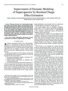
7.3 Design of the PMMSC As seen in Figure 11 both the control input u(k) and the Mach number response M(k) are used as inputs to the PMMSC. The control input is embedded in an m=50 dimensional space to represent the representative control sequences being applied to the tunnel. These control input sequences are clustered in C control classes (C=7). Here we use the available knowledge of operating the wind tunnel to select the representative control inputs to ramp the Mach number up and down and to regulate the set point. The most recent 50 samples of the control input are clustered to the closest representative control input (in a L1 norm sense). Two additional control classes which are only 10 samples long are used for identification purposes only. The winning cluster selects one of the 7 (C=0,1, … 6) SOM networks. The input to each of these SOM is obtained from the past history of the Mach number responses. An embed-

42-29

ding of the Mach number response in a space of N=50 is performed. Each of these SOM is trained in the full operating range of the Mach numbers and works as a codebook for the wind tunnel dynamics under the specified control input. Two additional SOMs, C=7,8, operate essentially in parallel on the m=10 subspace to identify the most recent input-output dynamics while ramping up or down. The size of each SOM here is 20 x 1, i.e. a linear array of PEs. This number of output PEs provided enough precision in the local linear models to achieve the required 0.003 tolerance in the Mach number [24]. Ensembles of Mach number responses resulting from the application of each control prototype were extracted from many hours of wind tunnel test data, sampled at 3 Hz (~2,000,000 samples or 40,000 vectors). Next, each ensemble of responses corresponding to one of the seven control prototypes was clustered using the SOM, trained over 10,000 epochs as explained in section 4.1. Each PE of the SOM is augmented with a local linear model as described in section 5, and the predictor trained as described in the same section. Figure 12 shows the weights of two converged SOM for the Mach number responses belonging to the two regulating control inputs. Notice the smooth organization of the weights across the neural field, from which the local linear models are derived. SOFM weights for input_class_6

SOFM weights for input_class_5

−3

x 10

−3

x 10

10 5

8

0

4

Delta Mach

Delta mach

6

2 0

−5

−10

−2 −4 20

−15 0

50

15 10

0

30 15

10 0

20

10

30 20

5 Cluster #

0 10

5

40

40 20

n

50

n

Cluster #

Figure 12. SOM for the Mach number responses of the regulating control prototypes The local linear model associated with each PE is used to predict the tunnel dynamics for the next 50 samples under the repertoire of our candidate control inputs. We developed a

42-30

family of 29 control waveforms, shown in Figure 13. Candidate Control Inputs u(t+n) 1

+1 Raise / −1 Lower

0.5

0

−0.5

−1 0 10 20 30 Candidate #

20

10

0

30

40

50

n

Figure 13. Repertoire of control inputs These control inputs are developed from experience with the goal of ramping up or down and regulating the Mach number. Each candidate control is fed to the local linear model of the winning PE producing a vector M of Mach number responses which is tested against the desired set point (Msp) within the last 30 points of the 50 point trajectory to emphasize steady state matching, i.e. 50

E =

å

M ( k ) – M sp ( k )

(32)

k = 21

The control input that produces the smallest Euclidean distance to the set point specification in steady state is elected as the best control, and sent to the controller. The control u(k) is updated every sample when ramping or steady-state control sequences are selected, but when regulatory control sequences are selected, the entire 50 sample control sequence is applied. Thus, when actively regulating about a set point, the switching between models is performed at most every 50 sample periods.

8. Experimental Control of the Wind Tunnel 8.1 Comparison of PPMSC Control to Existing Automatic Controller and Expert Operator

42-31

Figure 14 compares the regulating performance of the existing gain-scheduled control, an expert operator, and the PMMSC under similar conditions over a nominal fifteen minute interval. The first row of figures display the Mach numbers (with the +/-0.003 tolerance lines), followed by the control commands in the second row, and test model angle-ofattack (disturbance) for each of the three control schemes. The control commands are amplitude coded. Control commands whose duration is 0.3 seconds are displayed at amplitude 1. Control pulses of 0.1 second are shown with magnitude 0.33 and 0.2 second pulses are shown with magnitude 0.66. Control pulses of less than 0.1 second in duration are ineffective to produce a change in the fan drive rpm at any condition and are not used. Mach number @ 0.85 with NNCPC controller

Mach number @ 0.85 with operator control

0.856

0.854

0.854

0.854

0.852

0.852

0.852

0.85

0.848

0.846

Mean : 0.8497

Mach number

0.856

Mach number

Mach number

Mach number @ 0.85 with existing controller 0.856

0.85

0.848

5

Standard deviation : 0.001226

10

0.844

Out of tolerance : 34.52 seconds

2

15

4

6

8

Time (min)

10 Time (min)

12

14

16

0.6

0.6

0.6

0.4

0.4

0.4

0.2

0.2

0.2

Raise/Lower

1 0.8

Raise/Lower

1 0.8

−0.2

0 −0.2 −0.4

L1 norm: 10.63

0

−0.4

L1 norm: 12.33

−0.6

−0.6

−0.8

−0.8

−0.8

−1

5

10

15

2

4

6

8

10 Time (min)

12

14

16

−1 0

18

L1 norm: 6.33

5

10

15

10

15

Time (min)

Angle of Attack

Angle of attack (alpha)

15

−0.2

−0.6

−1 0

10

Commands from NNCPC control

1

0

5 Time (min)

Commands from operator

Commands from existing computer control

Out of tolerance : 33.23 seconds

0

18

0.8

−0.4

Mean : 0.8497

Standard deviation: 0.001358 0.844

Out of tolerance : 46.5 seconds

0

0.846

Mean : 0.8500

0.846

Standard deviation : 0.001527 0.844

0.85

0.848

Angle of attack (alpha)

14

14

14

12

12

12

10

10

8

8

10

6

Degrees

degrees

Degrees

8

6

6

4 4

4

2

2

0 0

0 0

2

5

10 Time (min)

15

0

2

4

6

8 10 Time (min)

12

14

16

18

−2 0

5 Time (min)

Figure 14. Comparison of the existing controller (left), expert operator(middle) and PMMSC (right). Derived metrics to quantify the comparisons between the three control strategies are the

42-32

time out of tolerance and the L1 norm of the control input, u(k). The time out of tolerance is the cumulative sum of time that the measured Mach number deviates beyond the required tolerance of 0.003: N

T out =

å α ∆t ( k )

(33)

k=1

where ì α = 0 M ( k ) – M sp ( k ) ≤ 0.003 í î α = 1 otherwise

(34)

and ∆t=t(k)-t(k-1). The L1 norm of the control command is L1 ( u ) =

N

å

u(k)

(35)

k=0

For this particular experiment, the angle-of-attack begins to mildly disturb the Mach number at approximately 5 degrees. Table 2 lists the reduction in the standard deviation of the Mach number, time out of tolerance, control effort, and time required to complete the sweep through the desired range of angle-of-attack while maintaining Mach number steady for this comparison. For this particular test condition, the PMMSC performs slightly better than the expert operator, but with much less control effort and less time to complete the alpha sweep. Compared to the existing automatic control, the PMMSC maintains the Mach number within the desired tolerance with less control effort, completing the alpha sweep in less time, which is the most important figure of merit for the utilization of the wind tunnel facility (relates to the time necessary to conduct the experiment). Table 2: Comparison of control schemes Controller (Cont)

Operator (Oper)

PMMSC

% reduction (Cont/Oper)

Mean

0.8497

0.8500

0.8497

-

SD

0.001527

0.001358

0.001226

20/10

Tout (sec)

46.5

34.52

33.2

29/4

L1

10.6

12.33

6.3

40/49

Alpha sweep (sec)

886

930

806

9/13

42-33

An additional metric on the control, the control density, was calculated by taking the sum of the absolute value of the control over a 50 sample sliding window: 49

å

ξ( k) =

u(k – i )

(36)

i=0

Control density for existing control

Control density for expert operator

4

4

3.5

3.5

3

3

2.5

2.5

2

2

1.5

1.5

1

1

0.5

0.5

0 0

2

4

6

8 Time (min)

10

12

14

16

0 0

Control density for NNCPC 4

3.5

3

2.5

2

1.5

1

0.5

2

4

6

8 10 Time (min)

12

14

16

18

0 0

2

4

6

8 Time (min)

10

12

14

16

Figure 15. Comparison of Control Densities (controller, operator, PMMSC) The control density is used to compare the sparseness of the control between the PMMSC, the existing controller, and an expert operator. This quantity measures the accuracy of the present control input so in the PMMSC case it is a measure of the accuracy of the local linear models to predict the tunnel dynamics. As illustrated in Figure 15, the PMMSC is clearly the most sparse, but allows for increased density of control when demanded by the external disturbance. In this respect it is similar to the variation in control density employed by the expert operator. This is in contrast to the existing automatic control, with fixed gains for a particular operating point resulting in a narrow range of control density. Figure 16 compares the result of controlling the Mach number to several different set points over a nominal 28 minute interval which involved operating point changes and regulation. The goal here is to show how the PMMSC handles ramping up and down the tunnel Mach number. Mach number set points of 0.95, 0.9, and 0.6 are common to all three controllers. The PMMSC controls the Mach number to the intermediate value of 0.85 instead of 0.8 for the operator and existing controller. This difference is minimal so this still provides a reasonable basis for comparison of the controllers. The angle-of-attack was varied extensively during all three runs. Again, the PMMSC maintains the Mach number within tolerance for a higher percentage of the time, with less expenditure of control effort. Table 3 lists the time out of tolerance and the L1 norm for the three runs. The PMMSC reduces the time out of tolerance on the order of 15-20 percent compared to the

42-34

existing automatic control or an expert operator. Table 3: Comparison for control schemes Controller

Operator

PMMSC

% reduction

Tout (sec)

329

310

266

19/16

L1 norm

424

466

374

12/20

Existing Control for set point changes

NNCPC control for set point changes

Setpoint changes under operator control

1

1

1

0.95

0.95

0.95

0.9

0.9

0.9 0.85

Out of tolerance: 328.8 sec 0.8

19.6 %

0.75

Mach number

0.85 Mach number

Mach number

0.85

0.8

0.8 0.75 Out of tolerance : 266.35 sec

0.75

0.7

15.9%

Out of tolerance: 310.2 sec 0.7

0.7

0.65

0.6 0

0.65

18.62%

0.6

0.65

5

10

15 Time (min)

20

25

0.6 0

30

5

10

15 Time (min)

20

25

30

0.55 0

1

0.8

0.8

25

30

1

L1 norm : 466.21

0.6

L1 norm: 374.27

0.2

0.2

0

0

−0.2

−0.2

−0.4

−0.4

−0.6

−0.6

−0.8

−0.8

5

10

15 Time (min)

20

25

0.4

Raise/Lower

0.4

Raise/Lower

Raise/Lower

20

L1 norm: 424.2

0.4

−1 0

15 Time (min)

0.8

0.6

0.6

10

NNCPC commands

Operator commands

Commands from existing control 1

5

−1 0

30

0.2 0 −0.2 −0.4 −0.6 −0.8

5

10

Angle of Attack

15 Time (min)

20

25

−1 0

30

10

15 Time (min)

20

25

30

Angle of Attack

Angle of Attack

10

5

12

8

10 6 8 5

6

0

degrees

Degrees

degrees

4

2

4 2 0

0

−2 −2 −4 −5 0

5

10

15 Time (min)

20

25

30

−4 0

5

10

15 Time (min)

20

25

30

−6 0

5

10

15 Time (min)

20

25

30

Figure 16. Comparison for controlling to several different set points (controller, operator, PMMSC).

9. Conclusions Nonlinear dynamical modeling is a rich area with many possible applications. Nonlinear

42-35

modeling seeks to estimate the nonlinear system that produced the time series under study. Hence it requires a nonlinear global model or a set of local linear models. Local linear modeling is conceptually elegant and requires mild assumptions about the underlying dynamics, but it is hindered by possible discontinuities among the local linear models. We propose an innovative modeling scheme based on a self-organizing map (SOM) which works not only as an enhanced clustering algorithm which preserves neighborhoods of the reconstruction space dynamics, but also as an estimator of the local linear models. We presented the mathematical principles that support the clustering model and derived a procedure to directly estimate the parameters of the local linear models from the SOM weights. The proposed enhanced SOM architecture implements naturally the necessary steps of identifying a nonlinear dynamical system from a time series. Our approach has several advantages: First, the SOM based modeling is computationally more efficient than other local models, which makes it very appealing for practical system identification applications. Second, since in our approach the SOM is trained globally to cluster the dynamics, the problem of discontinuities among the local models is reduced. In order to minimize the discontinuities, we applied a weighted least squares estimation to derive the local linear models. Third, we improved Kohonen learning for this task. The conventional Kohonen learning responds only to the density of samples in the input space, while here the fitting error to the trajectory is also important. Therefore we included an extra term in the Kohonen learning which assigns more PEs to regions of the trajectory where the error is larger. This improves the fidelity of the mapping. It is very interesting to observe that in the appropriately trained SOM for dynamic modeling, the trajectory of the winning PE in the output space describes a complicated path that is a projection of the reconstruction space trajectory. The beauty of the approach is that the complexity of the trajectory is naturally decomposed in the appropriate switching among very simple linear models, which leads to accurate dynamic modeling and very direct engineering applications in system identification and controls. Our proposed SOM approach is relevant for the switching controllers for two reasons: first it guaranteed that the repertoire of dynamics used for training the SOM are appropriately represented at the output of the SOM. Second, the same system that is performing the mapping is utilized to derive the local linear models, which makes the identification of the plant very compact and computationally efficient. In a sense, the diverse plant dynamics are captured in a compact look-up table of linear models. We applied this concept to the control of the NASA Langley transonic wind tunnel with

42-36

very good results. The control problem is one of regulating the set point of the plant under nonstationary loads (produced by the modification of the angle of attack of the aircraft model inside the tunnel). There are several peculiarities to this problem that made this solution so simple and accurate. First, the wind tunnel is stable, which means that the problem is one of regulation. Second, there is plenty of data to train a locally linear dynamic model of the tunnel dynamics under different load conditions. Third, the control input is a time series with 3 levels which enables a meaningful clustering of the control input is a small set of representative control commands. Hence we can discretize the control space, and simplify the modeling of the tunnel dynamics with the control input as a set of seven “different” wind tunnels. For each we modeled the dynamics with our proposed SOM approach. Once the selected SOM determines the winner PE the system has a local linear model of the plant which can be used to automatically predict the Mach number produced by a small, but effective, set of control commands. Hence the control command that best meets the set point is used as the next command input. Regulating around a set point is distilled into the selection of a local linear model that is used to predict the tunnel dynamics and determines which is the best possible control input (hence the name predictive multiple model switching controller PMMSC). The PMMSC is easily implemented for on-line operation in a 486 PC and was utilized to control the wind tunnel during 9 hours for 3 different aerodynamic modeling experiments. We demonstrated the accuracy of our controller during these runs and showed that it outperformed the existing controller and even trained operators. We realize that PMMSC is not a general control architecture. The PMMSC is set in advance, so it is not able to adjust to events that are very different from the ones used during training. But what is remarkable is that switching appropriately among a set of 140 local models was able to control to within 0.003 the Mach number of the wind tunnel during normal experimental conditions which create nonstationary loading. Very probably conditions different from the ones used to train the system were encountered during the 9 hour test runs, but as long as the new dynamics could be reasonably approximated locally by the developed dynamic code books the performance remained within bounds. This attests the power of local linear dynamic modeling, and of the proposed SOM based architecture. This reasoning also clearly points the direction of further work. Once we have this simple method of capturing a priori the dynamics about the task, the goal should be to integrate the SOM dynamic infrastructure in more complex control architectures such as the adaptive critics or adaptive controls. These methods tend to work with no a priori information and therefore are very slow to converge. Inclusion of the SOM will speed up

42-37

the convergence, preserving at the same time their characteristics of adapting to new situations.

Acknowledgments: This work was partially supported by NSF grant ECS-9510715 and ONR grant N00014-94-1-0858.

10. References [1] Abarbanel, H.D.I., R. Brown, J.J. Sidorowich, and L.S. Tsimring, “The analysis of Observed chaotic data in physical systems,” Rev. Mod. Phy., Vol. 65, No. 4, pp. 1331, 1993 [2] Ahalt, S.C., et al., “Competitive learning algorithms for vector quantization,” Neural Networks 3, pp. 277, 1990. [3] Box G. E. P., and Jenkins G. M., “Time series analysis: forecasting and control”, Holden-Day, 1976. [4] Broomhead D.S. and Lowe D., “Multivariate functional interpolation and adaptive networks”, Complex Systems 2, 321-355, 1988. [5] Bryant, P., R. Brown, and H.D.I. Abarbanel, “Lyapunov exponents from observed time series,” Phys. Rev. Lett. 65, pp. 1523, 1990. [6] Capone, F.J., Bangert, L.S., Asbury, S.C., Mills,C.T.L, Bare, E.A., The NASA Langley 16-Foot Tunnel, NASA Technical Paper 3521 , September 1995 [7] Casdagli, M., “Nonlinear prediction of chaotic time series,” Physics D 35, pp. 335, 1989. [8] Cherkassky, V., and H. Lari-Najafi, “Constrained Topological Mapping for Nonparametric Regression Analysis,” Neural Networks, Vol. 4, pp. 27, 1991. [9] Cherkassky V., Gehring D., Mulier F., “Comparison of adaptive methods for function estimation from samples”, IEEE Trans. Neural networks, vol 7, #4, 969-984, 1996. [10] Crutchfield, J.P., and B.S. McNamara, “Equations of motion from a Data Series,” Complex Systems 1, pp. 417, 1987. [11] Farmer, J.D., Sidorowich J.J., “Predicting chaotic time series,” Physical Review Letters, vol. 59, No. 8, pp. 845, 1987. [12] Giona, M., F. Lentini, and V. Cimagalli, “Functional reconstruction and local predic-

42-38

tion of chaotic time series,” Phys. Rev. A 44, pp. 3496-3502, 1991. [13] Grassberger, P. and I. Procaccia, “Characterization of strange attractors,” Physical Review Letters, Vol. 50, No. 5, pp. 346-349, 1983. [14] Guilleman, V., and A. Pollack, “Differential Topology”, Prentice-Hall, Englewood Cliffs, New Jersey, 1974. [15] Hammel, S.M., “A noise reduction method for chaotic systems,” Physics Letters A, 148, pp. 421, 1990. [16] Haykin S., and Principe J., “Dynamic modeling of chaotic time series with neural networks”, IEEE DSP Magazine, May issue, 1998. [17] Haykin, S., “Neural Networks: A Comprehensive Foundation”, Macmillan College Publishing, 1994. [18] Kohonen, T., “Self-organizing feature maps”, Springer Verlag, 1995. [19] Kohonen, T., “The self-organizing map,” Proceedings of the IEEE, Vol. 78, No. 9, 1990. [20] Kostelich, E.J., and J.A. Yorke, “Noise reduction: finding the simplest dynamical system consistent with the data,” Physica D, 41, pp. 183, 1990. [21] Lapedes, R., and R. Farber, “Nonlinear signal processing using neural networks: prediction and system modeling,” Technical Report LA-UR87-2662, Los Alamos National Laboratory, Los Alamos, New Mexico, 1987. [22] Luttrell, S.P., “Self-organization: A derivation from first priciples of a class of learning algorithms,” IEEE Conference on Neural Networks, pp. 495, Washington, DC, 1989. [23] Martinetz, T.M., S.G. Berkovich and K.J. Schulten, ““Neural-Gas” network for vector quantization and its application to time-series prediction,” IEEE Trans. on Neural Networks, Vol. 4, No. 4, July 1993. [24] Motter M., “Control of the NASA Transonic wind tunnel with the Self-Organizing Feature Map”, Ph.D. dissertation, University of Florida, Dec 1997. [25] Narendra, K.S. , Balakrishnan, J., and Ciliz, M.K., "Adaptation and Learning Using Multiple Models, Switching, and Tuning", in IEEE Control Systems Magazine, Vol.15, No. 3, 1995. [26] Narendra, K.S. , Balakrishnan, J., "Adaptive Control Using Multiple Models", in IEEE Transactions on Automatic Control, Vol.42, No. 2, pages 171-187, 1997. [27] Narendra, K.S. , Mukhopadhyay, S. , (1997). "Adaptive Control Using Neural Net-

42-39

works and Approximate Models", in IEEE Transactions on Neural Networks, Vol.8, No.3, pages 475-485. [28] Najai H., Cherkassky V., “Adaptive knot placement for nonparametric reression”, in Proc. Neural Inf. Proc. Systems, NIPS-6, 247-254, Morgan Kaufman, 1994 [29] Ott, E., C. Grebogi, and J.A. Yorke, “Controlling chaos,” Physical Review Letters, Vol. 64, No. 11, pp. 1196-1199, 1990. [30] Haykin S. and Li X. B., “Detection of signals in chaos,” Proceedings IEEE 83, 94122, 1995. [31] Packard, N.H., J.P. Crutchfield, J.D. Farmer, and R.S. Shaw, “Geometry from a time series,” Phys. Rev. Lett. 45, pp. 712, 1980. [32] Papoulis, A., “Probability, Random Variables, and Stochastic Processes”, 3rd ed., McGraw-Hill, New York, 1991. [33] Priestley, M.B., “State-Dependent Models: A general approach to nonlinear time series analysis,” Journal of Time Series Analysis, 1, pp. 47, 1980. [34] Principe, J.C. and Kuo J-M., “Dynamic modelling of chaotic time series with neural networks”, Proc. of Neural Infor. Proc. Sys, NIPS 7, 311-318, 1995. [35] Principe, J.C. and Wang L., “Non-linear time series modeling with self-organizing feature maps”, Proc. IEEE Workshop Neural Networks for Signal Proc., 11-20, 1995. [36] Principe J.C., Wang L., and J-M Kuo, “Chaotic time series modeling with neural networks”, in Signal Analysis and Prediction, Birkhauser, in Press. [37] Rissanen, J., “Stochastic Complexity in Statistical Inquiry”, World Scientific, 1989. [38] Ritter, H., “Learning with the self-organizing map,” In Artificial Neural Networks (T. Kohonen, K Makisara, O. Simula, and J. Kangas, eds.), Vol. 1, pp. 379-384, Amsterdam: North Holland, 1991. [39] Ritter H., “Parametrized self-organizing maps for vision tasks”, In Proc. ICANN’94, Italy, pp 803-810, 1994. [40] Sano, M., and Y. Sawada, “Measurement of the Lyapunov spectrum from a chaotic time series,” Physical Review Letters, Vol. 55, No. 10, pp. 1082, 1985. [41] Scharf, L.L., “Statistical Signal Processing--Detection, Estimation, and Time Series Analysis”, Addison-Wesley, 1989. [42] Shinbrot, T., E. Ott, C. Grebogi, and J.A. Yorke, “Using chaos to direct trajectories to targets,” Phys. Rev. Lett. 65, pp. 3250, 1990.

42-40

[43] Sidorowich, J.J., “Modeling of chaotic time series for prediction, interpolation, and smoothing,” IEEE ICASSP, 4, pp. 121, 1992. [44] Singer, A.C., Wornell G., Oppenheim A., “Codebook prediction: a nonlinear signal modeling paradigm,” IEEE ICASSP, 5, pp. 325, 1992. [45] Takens, F., “Detecting strange attractors in turbulence,” in Dynamical Systems and turbulence, ed. by D.A. Rand and L.-S. Young, Springer Lecture Notes in Mathematics, 898, pp. 365-381, Springer-Verlag, New York, 1980. [46] Goodwin, G.C., and K.S. Sin, “Adaptive filtering, prediction, and control”, PrenticeHall, 1984. [47] Tong, H., “Non-linear Time Series Analysis: A Dynamical Systems Approach”, Oxford University Press, Oxford, 1990. [48] Walter, J.“Non-linear prediction with self-organization maps,” IJCNN, I-589, 1990. [49] Walter J., Ritter H., “Local PSOMs and Chebyshev PSOMs improving the PSOM”, Proc Int. Conf. ANNs (ICANN95), vol 1, 95-102, 1995. [50] Walter J., Ritter H., “Rapid learning with parametrized self-organizing maps”, NeuroComputing 12, pp 131-153, 1996 [51] Wang, L., “Local linear dynamic modeling with self organizing feature maps”, Ph.D. Dissertation, U. of Florida, 1996. [52] Weigend, A.S., and N.A. Gershenfeld, “Time Series Prediction: Forecasting the future and understanding the past”, Addison-Wesley Publishing Company, 1984. [53] Widrow, B., and S.D. Stearns, “Adaptive Signal Processing”, Prentice-Hall, Englewood Cliffs, NJ, 1985. [54] Wolf, A., J.B. Swift, H.L. Swinney, and J.A. Vastano, “Determining Lyapunov exponents from a time series,” Physica D 16, pp. 285, 1985. [55] Vesanto J., “Using the SOM and local linear models in time series prediction”, Workshop on Self-Organizing Maps WSOM97, Helsinky, Finland, Aug 1997.

11. Appendix Let X , A and Φ denote the continuous input space, spatially discrete output space and a competitive projection respectively. The proposed non-linear modeling scenario follows three steps: a. Reconstruction of the state space from the input signal; b. Training the SOM; c. Estimation of the locally linear predictors.

42-41

* Reconstruction of the state space from the training signal. Embed the time series in a space of dimension N+1, where N is Takens’ embedding T dimension ( N ≥ 2D e ). A sequence of N+1 dimensional state vectors[ x ( n + τ ), x ( n ) ] is T created from the time series, where x ( n ) = [ x ( n ), x ( n – τ ), …, x ( n – ( N – 1 )τ ) ) ] and τ is the appropriate time delay. * Training the SOM model. This step is accomplished via the Kohonen learning process (or preferably with the T improved dynamic learning of section 5.1). With each vector-scalar pair [ x ( n + τ ), x ( n ) ] presented at the network input, train the system with Eq. 15. The learning process adapN+1 tively discretizes the continuous input space X ⊂ R into a set of K disjoint cells A to construct the mapping Φ: X → A . This process continues until the learning rate decreases close to zero and the neighborhood function covers about one output PE. After learning, the output space lattice A represents the input space X. The mapping Φ represents the input space data distribution and preserves local neighborhood relations. * Estimate the locally linear predictors. Once the SOM is trained, for each PE u i ∈ A , the corresponding local linear predictor coefficients [aiT, bi] are estimated based on α i ⊂ A , which is a set of NL elements in the neighborhood of ui including ui itself. Each element ui, has a corresponding weight vector T N+1 [ w i0, w ij ] ∈ R , where w ij = [ w i1, w i2, …, w iN ] . The local prediction T model [ai , bi] is fitted in the least-square sense to the set of weights in αi, i.e. T

w i0 = b i + a i w ij

(37)

To ensure a stable solution of the above equations, αi must have more than N+1 elements. Thereafter for each output unit u i ⊂ A , a unique linearly local model function ˜f ( a ( . ), b ( . ) ) is constructed. i i

42-42