Local Gaussian Regression

Local Gaussian Regression

arXiv:1402.0645v1 [cs.LG] 4 Feb 2014

Franziska Meier1 Philipp Hennig2 Stefan Schaal1,2 1 Computational Learning and Motor Control Lab, University of Southern California, Los Angeles 2 Max-Planck-Institute for Intelligent Systems, T¨ ubingen, Germany

Abstract Locally weighted regression was created as a nonparametric learning method that is computationally efficient, can learn from very large amounts of data and add data incrementally. An interesting feature of locally weighted regression is that it can work with spatially varying length scales, a beneficial property, for instance, in control problems. However, it does not provide a generative model for function values and requires training and test data to be generated identically, independently. Gaussian (process) regression, on the other hand, provides a fully generative model without significant formal requirements on the distribution of training data, but has much higher computational cost and usually works with one global scale per input dimension. Using a localising function basis and approximate inference techniques, we take Gaussian (process) regression to increasingly localised properties and toward the same computational complexity class as locally weighted regression.

1

Introduction

Besides expressivity and sample efficiency, computational cost is a crucial design criterion for machine learning algorithms in real-time settings, such as control problems. An example is the problem of building a model for robot dynamics: The sensors in a robot’s limbs can produce thousands of datapoints per second, quickly amassing a local coverage of the input domain. In such settings, fast local learning and generalization can be more important than a globally optimized model. A learning method should rapidly produce a good model from the large number N of datapoints, using a comparably small number M of parameters. Locally weighted regression (LWR) [1] makes use of the popular and well-studied idea of local learning [2] to address the task of compressing large amounts of data into a small number of parameters. In the spirit of a Taylor expansion, the idea of LWR is that simple models with few parameters may locally be precise,

while it may be difficult to find good nonlinear features to capture the entire function globally – lots of good local models may form a good global one. The key to LWRs low computational cost (linear, O(N M )) is that each local model is trained independently. The resulting speed has made LWR popular in robot learning. The downside is that LWR requires several tuning parameters, whose optimal values can be highly data dependent. This is at least partly a result of the strongly localized training strategy, which does not allow models to ‘coordinate’, or to benefit from other local models in their vicinity. Here, we explore a probabilistic alternative to LWR that alleviates the need for parameter tuning, but retains potential for fast training. An initial candidate could be the mixture of experts model (ME) [3]. Indeed, it has been argued [1], that LWR can be thought of as a mixture of experts model in which experts are trained independently of each other. The advantage of ME is that it comes with a full generative model [4, 5] allowing for principled learning of parameters and expert allocations, while LWR does not (see Figure 1). However, in this work we emulate LWRs assumption that the data is a continous function as opposed to a mixture of linear models, for instance. When the underlying data is not assumed to be generated by a mixture model, utilizing ME to fit the data makes inference (unneccesarily) complicated. Hence, we are interested in a probabilistic model that captures the best of both worlds without making the mixture assumption: A generative model that has the ability to localize computations to speed up learning. Our proposed solution is local Gaussian regression (LGR), a linear regression model that explicitly encodes localisation. Starting from the well-known probabilistic, Gaussian formulation of least-squares generalized linear regression, we first re-interpret the well known radial basis feature functions as localisers of constant feature functions. This allows us to introduce more expressive features, capturing the idea of local models within the Gaussian regression framework. In its exact form, this model has the cubic cost in M typical of


λm

λm

prediction

λm

prediction

prediction

N

training set

training set

K

∗ fm

xn fm

zxn

y∗

yxn

∗ αmk ξmk

xn ξmk

n φxmk

wmk

local models

∗ ξmk

xn ξmk

xn ξ˜mk

wmk

xn ηm

∗ fm

xn fm

xn y˜m

M

y∗

yxn

mixture of experts

φ∗mk

K

M z∗

∗ ηm

localizers

φ∗mk

wmk

xn ηm

localizers

αmk

n φxmk

local models

∗ ηm

localizers

local models xn ηm

training set

N

N

local Gaussian regression

yxn

∗ y˜m

∗ K ηm

M

y∗

locally weighted regression

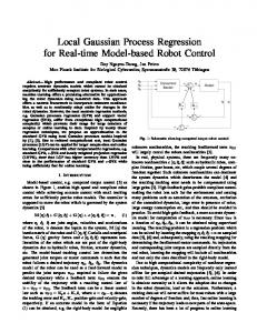
Figure 1: Generative model for mixture of experts (ME) (left), local Gaussian regression (LGR) (middle), and factor graph for locally weighted regression (LWR) (right). LWR assumes a fixed contribution of each local model to each observation. So a V-structure only exists within each m-plate, making inference cheaper. In ME, contributions of experts to each observations are normalized, coupling all the experts and making it necessary to update responsibilities in the e-step in a global manner. In local Gaussian regression, the contribution of each model to observations is uncertain (similar to ME), so the model is more densely connected than LWR. However, LWR is not a generative model for the data: It treats training and test data in different ways.

Gaussian models, arising because observations induce correlation between all local models in the posterior. To decouple the local models, we propose a variational approximation that gives essentially linear cost in the number of models M . The core of this work revolves around fitting the model parameters using maximum likelihood (Section 3.1). As a final note, we show how the novel feature function representation allows us to readily extend our probabilistic model to a local nonparametric formulation (Section 4). Previous work on probabilistic formulations of local regression [6, 7] has been focussed on bottom-up constructions, trying to find generative models for one local model at a time. To our knowledge, this is the first top-down approach, starting from a globally optimal training procedure, to find approximations giving a localized regression algorithm similar in spirit to LWR.

2

Background

Both LWR and Gaussian regression have been studied extensively before, so we only give brief introductions here. Generalized linear regression maps weights w ∈ RF to the nonlinear function f ∶ RD _ R via F feature functions φi (x) ∶ RD _ R: F

f (x) = ∑ φi (x)wi = φ w. i=1

⊺

(1)

Using the feature matrix Φ ∈ RN ×F whose elements are Φnf = φf (xn ), the function values at N locations xn ∈ RD , subsumed in the matrix X ∈ RN ×D , are f (X) = Φw. Locally weighted regression (LWR) trains M local regression models. We will assume each local model has K local feature functions ξmk (x), so that the m-th model’s prediction at x is K

fm (x) = ∑ ξmk (x)wmk = ξ m (x)wm

(2)

k=1

K = 2 and ξm1 (x) = 1, ξm2 (x) = (x − cm ) gives a linear model around cm . The models are localized by a nonnegative, symmetric and integrable weighting ηm (x), typically the radial basis function (x − cm )2 ] , or, for x ∈ RD , 2λ2m 1 ηm (x) = exp [− (x − cm )Λ−1 (x − cm )⊺ ] . 2 ηm (x) = exp [−

(3) (4)

with center cm and length scale λ or positive definite metric Λ. In LWR, each local model is trained independently of the others, by minimizing a quadratic

Franziska Meier1 , Philipp Hennig2 , Stefan Schaal1,2

loss

the posterior distribution is itself Gaussian: N

M

L(w) = ∑ ∑ ηm (xn )(yn − ξ m (xn )wm )2

(5)

n=1 m=1

N M √ √ 2 = ∑ ∑ ( ηm (xn )yn − ηm (xn )ξ m (xn )wm ) n=1 m=1

over the N observations (yn , xn ). At test time, local predictions (2) are combined into a joint prediction at input x as a normalised weighted sum ∑ ηm (x)fm (x) f (x) = m = ∑ φmk (x)wmk ∑m′ ηm′ (x) m,k

(6)

with the features φmk (x) =

ηm (x)ξmk (x) . ∑m′ ηm′ (x)

(7)

An important observation is that the objective (5) cannot be interpreted as least-squares estimation of the linear model Φ from Eq. (6). Eq. (5)√ is effectively training M linear models with φmk (xn ) = ηm (xn )ξmk (xn ) on √ M separate datasets ym (xn ) = ηm (xn )yn , but that model differs from the one in Equation (6). Thus, LWR can not be cast probabilistically as one generative model for training and test data simultaneously. The factor graph in Figure 1, right, shows this broken symmetry. Training LWR is linear in N and M , and cubic in K, since it involves a least-squares problem in the K weights wm . But this low cost profile also means absence of mixing terms between the M models, thus no ‘coordination’ between the local models. One problem this causes is that model-specific hyperparameters are not sufficiently identified and tend to over-fit. To pick one example among the hyperparameters: when learning the length scale parameters λm , there is no sense of global improvement. Each local model focusses only on fitting data points within a λm -neighborhood around cm . So the optimal choice is actually λ _ 0, which gives a useless regression model. To counteract this behaviour, implementations of LWR use regularisation of λ, but of course this introduces free parameters, whose best values are not obvious. Most works in LWR address this problem via leave-one-out cross-validation, which works well if the data is sparse. But when the data is dense, like in robotics, the kernel tends to shrink to only ‘activate’ points close by the left-out data point. Gaussian regression [8, §2] is a probabilistic framework for inference on the weights w given the features φ. Using a Gaussian prior p(w) = N (w; µ0 , Σ0 ) and a Gaussian likelihood p(y ∣ φ, w) = N (y; φ⊺ w, β −1 I),

p(w ∣ y, φ) = N (w; µN , ΣN ) µN =

ΣN =

(Σ−1 0 (Σ−1 0

with

+ βΦ Φ) (βΦ y ⊺

−1

+ βΦ Φ) ⊺

−1

⊺

− Σ−1 0 µ0 )

(8) (9) (10)

The mean of this Gaussian posterior is identical with the Σ-regularised least-squares estimator for w, so it could alternatively be derived as the minimiser of the loss function N

L(w) = w⊺ Σ−1 w + ∑ (yn − φ(xn )w)2 .

(11)

n=1

But the probabilistic interpretation of Equation (8) has additional value over (11) because it is a generative model for all (training and test) data points y, which can be used to learn hyperparameters of the feature functions. The prediction for f (x∗ ) with features φ(x∗ ) =∶ φ∗ is also Gaussian, with p(f (x∗ ) ∣ y, φ) = N (f (x∗ ); φ∗ µN , φ∗ ΣN φ⊺∗ )

(12)

As is widely known, this framework can be extended to the nonparametric case by a limit which replaces all inner products φ(x1 )Σ0 φ(x2 )⊺ with a Mercer (positive semi-definite) kernel function k(x1 , x2 ). The corresponding priors are Gaussian processes. This generalisation will only play a role in Section 4 of this paper, but the direct connection between Gaussian regression and the elegant theory of Gaussian processes is often cited in favour of this framework. Its main downside, relative to LWR, is computational cost: Calculating the posterior (12) requires solving the least-squares problem for all F parameters w jointly, by inverting ⊺ the Gram matrix (Σ−1 0 + βΦ Φ). In the general case, 3 this inversion requires Ø(F ) operations. The point of the construction in the following sections is to use approximations to lower the computation cost of this operation such that the resulting algorithm is comparable in cost to LWR, while retaining the probabilistic interpretation, and the modelling robustness of the full Gaussian model. The Gaussian regression framework puts virtually no limit on the choice of basis functions φ, even allowing discontinuous and unbounded functions, but the radial basis function (RBF, aka. Gaussian, squareexponential) features from Equation (3), φi (x) = η i (x), (for F = M ) enjoy particular popularity for various reasons, including algebraic conveniences and the fact that their associated reproducing kernel Hilbert space lies dense in the space of continuous functions [9]. A downside of this covariance function is that it uses one global length scale for the entire input domain. There are some special kernels of locally varying regularity [10], and mixture descriptions offer a more discretely varying model class [11]. Both, however, require computationally demanding training.


2

2

2

1

1

1

0

0

0

−1

−1

−1

−2 2

−2 2

−2

1

1

1

0

0.2

0.4

0.6

0.8

1

0

0.2

0.4

0.6

0.8

1

0

0

0

−1

−1

−1

−2

0

0.2

0.4

(a)

0.6

0.8

1

−2

0

0.2

0.4

0.6

0.8

1

0

0.2

0.4

0.6

0.8

1

2

0

0.2

0.4

0.6

(b)

0.8

1

−2

(c)

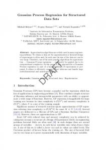
Figure 2: Noisy data drawn from sine function learned by (a) LWR (b) exact and (c) approximate local Gaussian regression. In LWR, local models do not know of each other and thus fit tangential lines around the center of each local model. In local Gaussian regression local models are correlated. They work together to fit the function. In the approximate version (c) this correlation is reduced, but not completely gone.

3

Local Parametric Gaussian Regression

factorizing prior M

In Gaussian regression with RBF features as described above, without changing anything, the features φm (x) = ηm (x) can be interpreted as M constant function models ξm (x) = 1, localised by the RBF function, φ(x) = [ξ1 (x)η1 (x), . . . , ξM (x)ηM (x)]. This representation extends to more elaborate local models ξ(x). For example ξ(x) = x gives a local weighted regression with linear local models. Extending to M local models consisting of K parameters each, feature function φnmk combines the k th component of the local model ξkm (xn ), localised by the m-th weighting function ηm (x) φnmk

∶= φmk (xn ) = ηm (xn )ξkm (xn ).

(13)

For these features, treating mk as the index set of a vector with M K elements, the results from Equations (8) and (12) apply, giving a localised linear Gaussian regression algorithm. The choice of local parametric model is essentially arbitrary. But regular features are an obvious choice. A scalar polynomial model of order K − 1 arises from ξkm (xn ) = (xn − cm )k−1 . Local linear regression in a Kdimensional input space takes the form ξkm (xn ) = xnk − cm . We will adopt this latter model in the remainder, because it is also the most widely used model in LWR. An illustration of LWR regression and the proposed local Gaussian regression is given in Figure 2. Since it will become necessary to prune out unnecessary parts of the model, we adopt the classic idea of automatic relevance determination [12, 13] using a

p(w∣A) = ∏ N (wm ; 0, A−1 m)

with

(14)

m=1

Am = diag(αm1 , . . . , αmK ).

(15)

So every component k of each local model m has its own precision, and can thus be pruned out by setting αmk _ ∞. Section 3.1 assumes a fixed number M of local models with fixed centers cm . Thus the parameters are θ = {β, {αmk }, {λmk }}. We propose an approximation for estimating these parameters. Section 3.2 then describes placing the local models incrementally to adapt M and cm . 3.1

Learning in Local Bayesian Linear Regression

Exact inference in Gaussian regression with localised feature functions comes with the cubic cost of its nonlocal origins. However, because of the localised feature functions, correlation between far away local models is approximately 0, hence inference is approximately independent between local models. In this section we aim to make use of this “almost independence” to derive a localised approximate inference scheme of low cost, similar in spirit to LWR. To arrive at this localised learning algorithm we first introduce a latent variable fnm for each local model m and data point xn , similar to probabilistic backfitting [14]. Intuitively, the f form approximate targets, one for each local model, against which the local regression parameters fit (see also Figure 1, middle). This modified model motivates a factorizing variational bound constructed in Section 3.1.1, rendering the the


local models computationally independent, which allows for fast approximate inference in the local Gaussian model. Hyperparameters will be learnt by approximate maximum likelihood (3.1.2), i.e. iterating between constructing a bound q(z ∣ θ) on the posterior over variables z given current parameter estimates θ and optimising q with respect to θ.

where Σf = B −1 − B −1 1(βy−1 + 1T B −1 1)−1 1T B −1 = B −1 − M

B −1 11T B −1 βy−1 + 1T B −1 1

µf n = ∑ Ew [wTm ] φ(xn )+

(22) (23)

m=1

3.1.1

Variational Bound

M 1 T −1 B 1 (y − E [wm ] φnm ) ∑ n ⊺ βy−1 + 1 B −1 1 m=1

The complete data likelihood of the modified model is N

p(y,f , w ∣ Φ, θ) = ∏ p(yn ∣ f n , βy )

(16)

n=1

N

M

M

n ∏ ∏ p(fnm ∣ φm wm , βf m ) ∏ p(wm ∣ Am )

n=1 m=1

m=1

(c.f. Figure 1, left). Our Gaussian model involves the latent variables w and f , the precision β and the model parameters λm , cm . We treat w and f as probabilistic variables and estimate θ = {β, λ, c}. On w, f , we construct a variational bound q(w, f ) imposing factorisation q(w, f ) = q(w)q(f ). The variational free energy is a lower bound on the log evidence for the observations y: log p(y ∣ θ) ≥ ∫ q(w, f ) log

p(y, w, f ∣ θ) . q(w, f )

(17)

This bound is maximized by the q(w, f ) minimizing the relative entropy DKL [q(w, f )∥p(w, f ∣ y, θ)], the distribution for which log q(w) = Ef [log p(y ∣ f , w)p(w, f )] and log q(f ) = Ew [log p(y ∣ f , w)p(w, f )]. It is relatively straightforward to show (e.g. [15]) that these distributions are Gaussian in both w and f .The approximation on w is log q(w) = Ef [log p(f n ∣ φ(xn ), w) + log p(w ∣ A)] M

= log ∏ N (wm ; µwm , Σwm )

(18)

m=1

where

N

−1

Σwm = (βf m ∑ φnm φnm + Am ) T

n=1

N

µwm = βf m Σwm ( ∑ φnm E [fnm ]) n=1

∈ RK×K ∈ RK×1

(19) (20)

The posterior update equations for the weights are local: each of the local models updates its parameters independently. This comes at the cost of having to update the belief over the variables fnm , which achieves a coupling between the local models. The Gaussian variational bound on f is log q(f n ) =

Ew [log p(yn ∣ f n , βy ) + log p(f n ∣ φnm , w)]

= N (f n ; µf n , Σf )

(21)

where µf n ∈ RM and using B = diag (βf 1 , . . . , βf M ). These updates can be performed in O(M K). Inspecting Equations (23) and (20), one can see that the optimal assignment of all µw actually amounts to a joint linear problem of size M K × M K, which could also be solved as a linear program. However, this would come at additional computational cost. 3.1.2

Optimizing Hyperparameters

We set the model parameters θ = {βy , {βf m , λm }M m=1 , {αmk }} to maximize the expected complete log likelihood under the variational bound, Ef ,w [log p(y, f , w ∣ Φ, θ)] =

(24)

N

M

n=1

m=1

Ef ,w { ∑ [ log N (yn ; ∑ fnm , βy−1 ) M

+ ∑ log N (fnm ; wTm φnm , βf−1m )] m=1 M

+ ∑ log N (wm ; 0, A−1 m )} m=1

Setting the gradient of this expression to zero leads to the following update equations for the variances βy−1 =

βf−1m =

1 N 2 T ∑ (yn − 1µf n ) + 1 Σf 1 N n=1

(25)

1 N n 2 nT n 2 ∑ [(µf nm − µwm φm ) + φm Σwm φm ] + σf m N n=1 (26)

−1 αmk = µ2wmk + Σw,kk

(27)

The gradient with respect to the scales of each local model is completely localized ∂Ef ,w [log p(y, f , w ∣ Φ, θ)] ∂ log λmk =

T −1 ∂Ef ,w [∑N n=1 N (fnm ; w m φm (xn ), βf m )]

∂λmk

(28)

We use gradient ascent to optimize the length scales λmk . All necessary equations are of low cost and, with


the exception of the variance β1y , all hyper-parameter updates are solved independently for each local model, similar to LWR. In contrast to LWR, however, these local updates do not cause a shrinking in the length scales: In LWR, both inputs and outputs are weighted by the localizing function, thus reducing the length scale improves the fit. The localization of Equation (13) only affects the influence of regression model m, but the targets still need to be fit accordingly. Shrinking of local models only happens if it actually improves the fit against the unweighted targets fnm . 3.1.3

Prediction at a test point x∗ arise from marginalizing over both w and f , using ∫ N (y∗ ; 1

f ∗ , βy−1 )N (f ∗ ; W T φ(x∗ ), B −1 )df∗

= N (y∗ ; ∑ wTm φ∗m , βy−1 + 1T B −1 1)

and

// initialize first local model

1: M = 1; c1 = x1 ; C = {c1 } // iterate over all data points

2: for n = 2 . . . N do 3: if ηm (xn ) < wgen , ∀m = 1, . . . , M then 4: cm ^ xn 5: C ^ C ∪ {cm }, M = M + 1 6: end if // E-Step: equations (19),(20),(22),(23)

{µwm , Σwm , µf m , Σf m }m ^ e-step({βy , βf m , {αmk , λmk }k }m )

7: 8:

Prediction

T

Algorithm 1 Incremental LGR Require: {xn , yn }N n=1

(29)

m

T ∗ −1 T −1 ∫ N (y∗ ;w φ , βy + 1 B 1)N (w; µw , Σw )dw M

= N (y∗ ; ∑ µTwm φ∗m , σ 2 (x∗ ))

// M-Step: equations (25),(26),(27),(28)

{βy , βf m , {αmk , λmk }k }m ^ m-step ({µwm , Σwm , µf m , Σf m }m )

9: 10:

// pruning

11: for all m do 12: if αmk > 1e3 ∀k = 1, . . . , K then 13: M ^ M − 1; C ^ C ∖ cm 14: end if 15: end for 16: end for

4

Extension to Finitely Many Local Nonparametric Models

(30)

m

where M

M

m=1

m=1

σ 2 (x∗ ) = βy−1 + ∑ βf−1m + ∑ φ∗m Σwm φ∗m T

(31)

which is linear in M and K. 3.2

Incremental Adding of Local Models

Up to here, the number M and locations c of local models were fixed. An extension analogous to the incremental learning of the relevance vector machine [16] can be used to iteratively add local models at new, greedily selected locations cM +1 . The resulting algorithm starts with one local model, and per iteration adds one local model in the variational step. Conversely, existing local models for which all components αmk _ ∞ are pruned out. This works well in practice, with the caveat that the number local models M can grow fast initially before the pruning becomes effective. Thus we check for each selected location cM +1 whether any of the existing local models c1∶M produces a localizing weight ηm (cM +1 ) ≥ wgen , where wgen is a parameter between 0 and 1 and regulates how many parameters are added. An overview of the final algorithm is given in 1.

An interesting component of local Gaussian regression is that it easily extends to a model with finitely many local nonparametric, Gaussian process models. Marginalising out the weights wm in Eq. (17) gives the marginal M

p(y, f ∣ X, θ) = N (y; 1⊺ f , βy−1 IN ) ∏ N (f m ; 0, Cm ) m=1

(32) where p(fm ) = N (f m ; 0, Cm ) is a Gaussian process prior over function fm with a (degenerate) covariance function Cm = βf−1m IN + φTm A−1 Rem φm . placing the finitely many local features ξm with infinitely many features results in the local nonparametric model with covariance function κm (x, x′ ) = βf−1m δij + ηm (x)ˆ κm (x, x′ )ηm (x′ ). The exact posterior over f x ∶= f (x) is with

p(f x ∣ y) = N (f x ; µx , Σxx )

m r ′ Σmr xx′ = cov(f (x), f (x ))

(33)

(34)

M

m m s −1 −1 r = δmr kxx kXx′ ′ − kxX (∑ kXX + βy I)

(35)

s

M

m s −1 −1 µm x = kxX (∑ kXX + βy I) y s

(36)


1

1

1

0

0

0

−1

−1

−1

1 0 1 0

−1−1

0

1

−2

(a)

−1

0

1

2

−2

(b)

−1

0

1

2

−2

(c)

−1

0

1

2

(d)

Figure 3: (a) 2D cross function, local models learnt by (b) LWPR, (c) LGR and (d) ME . Table 1: Predictive performance on Cross Function nMSE w/o LSL

opt wgen

# of LMs

nMSE with LSL

opt wgen

# of LMs

0.234 0.069 0.169

0.2 1.0 0.5

13 23.8 21.2

0.0365 0.0137 0.0313

0.1 0.9 0.4

45.5 23.3 62.2

LWPR GLR ME

So computing the posterior covariance Σmr xx′ requires one inversion of an N ×N matrix. It remains to be seen to what extend variational bounds on the parametric forms presented in the previous sections can be transported to a local nonparametric Gaussian regression framework.

5

Experiments

We evaluate and compare to mixture of experts and locally weighted projection regression (LWPR) – an extension of LWR suitable for regression in high dimensional space [17] – on two data sets. The first is data drawn from the “cross function” in Figure 3, often used to demonstrate locally weighted learning. For the second comparison we learn inverse dynamics of a SARCOS anthropomorphic robot arm with seven degrees of freedom [8]. In order to compare to mixture of experts we assume linear expert models. A prior of the form N (wm ; 0, A−1 m) on each experts regression parameters and normalized gaussian kernels for the mixture components are used in our implementation to make it as comparable as possible. To compute the posterior in the e-step a mean field approximation is employed. In both experiments, LWPR performed multiple cycles through the data sets. Both the local Gaussian regression and the mixture of experts implementation are executed based on Algorithm 1 and are allowed an additional 1000 iterations to reach convergence.

5.1

Data from the ‘Cross Function’

We used 2, 000 uniformly distributed training inputs, with zero mean Gaussian noise of variance (0.2)2 . The test set is a regular grid of 1641 edges without noise and is used to evaluate how well the underlying function is captured. The initial length scale was set to λm = 0.3, ∀m, and we ran each method with and without lengthscale learning (LSL) for wgen = 0.1, 0.2, . . . , 1.0. All results presented here are results averaged over 5 randomly seeded runs. Table 1 presents the top performance achieved by each method, including what the optimal setting for wgen was and how many local models were used. In both settings (with or without LSL) LGR outperforms both LWPR and ME in terms of accuracy as well as number of local models used. To understand the role of parameter wgen better, we also summarize the normalized mean squared error as a function of parameter wgen for all 3 methods in Figure 4 with (right) and without (left) LSL. The key message of this graph is that the parameter wgen does not affect the performance of LGR greatly. While accuracy slightly improves with increasing wgen it is not dramatic. Thus for LGR wgen can be thought of as a trade-off parameter, for smaller wgen the algorithm has to consider less potential local models, for a slight performance decrease. For LWPR and ME this relationship to wgen is not that clear. Furthermore, although LGR has to consider more local models for larger wgen (up to 2000 for wgen = 1), we only see a slight increase in the number of local models in the final model, indicating that the pruning mechanism works very well.


normalized MSE

M

train LWPR 200 150 100 50 0

0.1

0.2

0.3

0.4

test LWPR

0.5

0.6

0.7

0.8

train ME

0.9

1

200 150 100 50 0

test ME

0.1

0.2

train LGR

0.3

0.4

0.5

wgen 0.6

0.4

0.4

0.2

0.2 0.1

0.2

0.3

0.4

0.5

0.6

0.7

0.8

0.9

1

0.7

0.8

0.9

1

wgen

0.6

0

0.6

test LGR

0.7

0.8

0.9

0

1

0.1

0.2

0.3

0.4

0.5

wgen

0.6

wgen

Figure 4: normalized mean squared error (nMSE) on 2D cross data without (left) and with (right) lengthscale learning. Table 2: Predictive Performance on SARCOS task LWPR nMSE J1 J2 J3 J4 J5 J6 J7

0.045 0.039 0.034 0.024 0.064 0.075 0.03

(MSE)

(19.160) (8.938) (3.420) 4.552 (0.060) (0.221) (0.203)

LGR # of LM

nMSE

419 493 483 384 514 519 405

0.015 0.0195 0.014 0.016 0.035 0.027 0.023

(6.282) (4.391) (1.382) (3.118) (0.0336) (0.0786) (0.1578)

Finally, we show representative results of the shape of learned local models for LWPR, LGR and ME In Figure 3, nicely illustrating the key difference between the three methods: In LWPR local models don’t know of each other and thus aim to find the best linear approximation to the function. In both ME and LGR, the local models know of each other and collaborate to fit the function. 5.2

(MSE)

Inverse Dynamics Learning Task

The SARCOS data contains 44, 484 training data points and 4, 449 test data points. The 21 input variables represent joint positions, velocities and accelerations for the 7 joints. The task is to predict the 7 joint torques. In Table 2 we show the predictive performance of LWPR, ME and LGR when trained with lengthscale learning and with wgen = 0.3. LGR outperforms LWPR and ME in terms of accuracy for almost all joints.However, the true advantage of LGR lies in the fact the number of hand tuned parameters is reduced to setting the learning rate for the gradient descent updates and setting the parameter wgen .

6

ME # of LM

nMSE

(MSE)

# of LM

366 361 359 348 354 359 358

0.071 0.0871 0.074 0.039 0.058 0.124 0.0235

(30.125) (19.564) (7.319) (7.348) (0.0552) (0.363) (0.1589)

249 257 243 239 438 234 383

Conclusion

We have taken a top-down approach to developing a probabilistic localised regression algorithm: We start with the generative model of Gaussian generalized linear regression, which amounts to a fully connected graph and thus has cubic inference cost. To break down the computational cost of inference, we first introduce the idea of localised feature functions as local models, which can be extended to local nonparametric models. In as second step, we argue that because of the localisation these local models are approximately independent . We exploit that fact through a variational approximation that reduced computational complexity to local computations. Empirical evaluation suggests that LGR successfully addresses the problem of fitting hyperparameters inherent in locally weighted regression. A final step left for future work is to re-formulate our algorithm into an incremental version that can deal with a continuous stream of incoming data.


References [1] Stefan Schaal and Christopher G Atkeson. Constructive incremental learning from only local information. Neural Computation, 10(8):2047–2084, 1998. [2] L´eon Bottou and Vladimir Vapnik. Local learning algorithms. Neural computation, 4(6):888–900, 1992. [3] Robert A Jacobs, Michael I Jordan, Steven J Nowlan, and Geoffrey E Hinton. Adaptive mixtures of local experts. Neural computation, 3(1):79–87, 1991. [4] Steve Waterhouse, David MacKay, and Tony Robinson. Bayesian methods for mixtures of experts. Advances in neural information processing systems, pages 351–357, 1996. [5] Lauren Hannah, David M Blei, and Warren B Powell. Dirichlet process mixtures of generalized linear models. Journal of Machine Learning Research, 12:1923–1953, 2011. [6] Jo-Anne Ting, Mrinal Kalakrishnan, Sethu Vijayakumar, and Stefan Schaal. Bayesian Kernel Shaping for Learning Control. In Neural information processing systems, 2008. [7] Narayanan U Edakunni, Stefan Schaal, and Sethu Vijayakumar. Kernel carpentry for online regression using randomly varying coefficient model. In Proceedings of the international joint conference on artificial intelligence (IJCAI), 2007. [8] C.E. Rasmussen and C.K.I. Williams. Gaussian Processes for Machine Learning. MIT Press, 2006. [9] C.A. Micchelli, Y. Xu, and H. Zhang. Universal kernels. Journal of Machine Learning Research, 7:2651–2667, 2006. [10] M. N Gibbs. Bayesian Gaussian processes for regression and classification. PhD thesis, University of Cambridge, 1997. [11] C.E. Rasmussen and Z. Ghahramani. Infinite mixtures of Gaussian process experts. In Advances in neural information processing systems. MIT Press, 2002. [12] R.M. Neal. Bayesian learning for neural networks. Springer Verlag, 1996. [13] M.E. Tipping. Sparse Bayesian learning and the relevance vector machine. The Journal of Machine Learning Research, 1:211–244, 2001. [14] Aaron D’Souza, Sethu Vijayakumar, and Stefan Schaal. The bayesian backfitting relevance vector machine. In Proceedings of the twenty-first international conference on Machine learning, page 31. ACM, 2004. [15] M.K. Titsias. Variational learning of inducing variables in sparse Gaussian processes. In Artificial Intelligence & Statistics (AISTATS), volume 12, 2009. [16] Joaquin Quinonero-Candela and Ole Winther. Incremental gaussian processes. In Advances in neural information processing systems, pages 1001–1008, 2002.

[17] Sethu Vijayakumar and Stefan Schaal. Locally weighted projection regression: An o (n) algorithm for incremental real time learning in high dimensional space. In Proceedings of the Seventeenth International Conference on Machine Learning (ICML 2000), volume 1, pages 288–293, 2000.