Heteroscedastic Gaussian Process Regression for Modeling Range Sensors in Mobile Robotics. Christian Plagemann, Kristian Kersting, Patrick Pfaff, Wolfram ...
Heteroscedastic Gaussian Process Regression for Modeling Range Sensors in Mobile Robotics Christian Plagemann, Kristian Kersting, Patrick Pfaff, Wolfram Burgard Univ. of Freiburg, Dept. of Computer Science, D-79110 Freiburg, Germany {plagem,kersting,pfaff,burgard}@informatik.uni-freiburg.de
In probabilistic approaches to mobile robot navigation, the development of measurement models plays a crucial role as it directly influences the efficiency and the robustness of the robot’s performance in a great variety of tasks including localization, tracking, and map building [1]. Among the most popular types of sensors used are range finders, which measure distances to nearby obstacles relative to certain (possibly multivariate) bearing angles. Probabilistic measurement models for this kind of sensor, such as beam models (aka. ray-casting models) and likelihood fields (aka. end point models), typically assume independency between individual range measurements. This leads to a series of practical limitations such as overly peaked observation likelihood functions for high density range scans or degrading performance in highly cluttered environments. To overcome this, we propose a novel probabilistic measurement model for range finders, called Gaussian Beam Processes. Gaussian Beam Processes treat the measurement modeling task as a nonparametric Bayesian regression problem and solve it using Gaussian processes [2]. The major advantage of this approach lies in the smoothness of the model, resulting from the representation of correlations between adjacent beams using covariance functions. Moreover, the Gaussian process treatment results in a sound probabilistic measurement model with a pool of well-established techniques for likelihood estimation and range prediction for an arbitrary number of beams. Standard Gaussian processes, however, assume a constant noise term over the domain. For modeling range sensor measurements, the variance of range values in each beam direction is, along with its mean value, an important feature of the sought-after distribution of range measurements. Inspired by Goldberg et al. [3], we therefore extended the standard Gaussian process framework to deal with heteroscedasticity, i.e., non-constant noise. Like Goldberg et al., we model the log noise variances explicitly using a second Gaussian process. In contrast to their work, however, we do not use a time consuming Markov chain Monte Carlo method to estimate the posterior noise variances but a fast most-likely-noise approach. We implemented the proposed system and evaluated it using a real robot as well as simulation for one of the classical tasks of robotics, namely mobile robot localization. The experimental results using a particle filter for mobile robot localization demonstrate the effectiveness of Gaussian Beam Processes in comparison to previous approaches. Topic: Robotics Preference: Oral
References [1] S. Thrun, W. Burgard, and D. Fox, Probabilistic Robotics. MIT Press, 2005. [2] C. K. I. Williams and C. E. Rasmussen, “Gaussian processes for regression,” in Proc. of the Conf. on Neural Information Processing Systems (NIPS), D. S. Touretzky, M. Mozer, and M. E. Hasselmo, Eds. MIT Press, 1995, pp. 514–520. [3] P. W. Goldberg, C. K. I. Williams, and C. M. Bishop, “Regression with input-dependent noise: A gaussian process treatment,” in Advances in Neural Information Processing Systems, M. I. Jordan, M. J. Kearns, and S. A. Solla, Eds., vol. 10. The MIT Press, 1998.
1
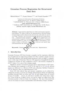
GP Model Ray Cast Model End Point Model
success rate [%]
100 80 60 40 20 0 10000
15000
20000
25000
30000
number of particles
Figure 1: Standard GP regression (left) assuming constant noise and our heteroscedastic extension (middle) dealing with non-constant noise. Scales are given in meters. The concentric lines depict possible range measurements. Modeling heteroscedasticity yields lower predictive uncertainties at places with low expected noise levels such as the walls in front. The right plot depicts the ratio of successful localizations of a real robot after 8 integrations of measurements for a varying number of particles. As can be seen from the diagram, our Gaussian Beam Process model increases the global localization performance compared to state of the art approaches. Baseline (random likelihoods) RC LF GBP
4 3.5
KL-Divergence to ground truth
KL-Divergence to ground truth
4.5
3 2.5 2 1.5 1 0.5
Baseline (random likelihoods) RC LF GBP
2.25 2 1.75 1.5 1.25 1 0.75 0.5 0.25 0
0 10
20
30
40
50
60
70
80
0
50
Number of test beams
100
150
200
250
Number of test beams
Figure 2: Localization performance for a mobile robot in terms of the Kullback-Leibler divergence (KLD), which measures the distance of the discretized pose belief distribution to the known ground truth (lower values are better). The experiments were simulated in an office (left) and in a cluttered environment (right). The KLD (y-axis) is shown for a varying number of laser beams (x-axis). The baseline model (uniform) assigns the same log likelihoods to all possible poses. In the office environment (left), all methods perform similarly well. In the highly cluttered environment, however, Gaussian Beam Processes significantly outperform the others. The error bars indicate the standard deviations from 10 independent runs. 2
GP Model Ray Cast Model End Point Model
average translation error
average translation error
2
1.5
1
0.5
0
GP Model Ray Cast Model End Point Model
1.5
1
0.5
0 0
200
400
600
800
0
iteration step
200
400
600
800
iteration step
Figure 3: Pose tracking results for a real robot in an office environment using an 180 degrees field of view. The tracking displacement errors (y-axis) in meters are given for an increasing number of iterations (x-axis) using 31 laser beams (left) and 61 laser beams (right). The errors are averaged over 25 runs on the same trajectory. As can be seen from the right diagram, the ray cast model often leads to divergence for larger numbers of beams. 2