accuracy of NB models when compared to traditional max- imum likelihood .... sick. 29. 2. 3772 tumor. 17. 22. 339 hypothyroid 29. 4. 3772 ionosphere. 34. 2. 351.
2009 Fourth International Conference on Innovative Computing, Information and Control
Local-Global-Learning of Naive Bayesian Classifier Shengtong Zhong, Helge Langseth Department of Computer and Information Science Norwegian University of Science and Technology NO-7491 Trondheim, Norway {shket, helgel}@idi.ntnu.no denote the class variable with m classes. The NB classifier select the most likely classification of instance a as:
Abstract Naive Bayes (NB) models are among the simplest probabilistic classifiers. However, they often perform surprisingly well in practice, even though they are based on the strong assumption that all attributes are conditionally independent given the class variable. The vast majority of research on NB models assume that the conditional probability tables in the model are either learned by maximum likelihood or Bayesian methods, even though it is well documented that learning NB models in this way may harm the expressiveness of the models. In this paper, we focus on an alternative technique for learning the conditional probability tables from data. Instead of frequency counting (which leads to maximum likelihood parameters), we propose a learning method that we call ”local-global-learning”. We learn the (local) conditional probability tables under the guidance of the (global) NB model learnt thus far. The conditional probabilities learned by local-global-learning are therefore geared towards maximizing the classification accuracy of the models instead of maximizing the likelihood of the training data. We show through extensive experiments that localglobal-learning can significantly improve the classification accuracy of NB models when compared to traditional maximum likelihood learning.
Figure 1. Naive Bayes models
∗
C (a) = arg max P (C = c) c
P (ai |c)
(1)
i=1
As all attributes are conditionally independent given the class variable, the classifier is determined by P (C = c), the probability distribution of class variable, and P (ai |c), the local probability distribution for each attribute. The local distribution is specified by a conditional probability table (CPT). The vast majority of research on NB models assume that the CPT in the model are either learned by maximum likelihood or Bayesian methods. In general, maximum likelihood inference is simply achieved by frequency counting when learning a CPT for the NB classifier, and thus is a typical generative learning method. Jaeger [5] showed that a NB model can recognize any linearly separably concept, and argues that previous results of representation power for the NB models [2] are due to these authors assuming that all learning are based on the maximum likelihood principle. This indicates that other learning paradigms may lead to better classification accuracy than maximum likelihood learning. Further evidence for this idea is given by Ng & Jordan [4], who showed that discriminative classifiers work better than generative classifiers when there is no missing data, and particularly for small data sets. In classification, the object is to maximize classification accuracy, rather than maximum likelihood. Hence, it may be beneficial to consider learning CPT with discriminative method, as this could improve the
1. Introduction Naive Bayes (NB) models have the strong assumption that all attributes are conditionally independent given the class variable (Figure 1). Even though NB models are among the simplest probabilistic classifiers, they often perform surprisingly well in practice. When learning a NB classifier, the classifier is constructed from a given set of labeled training instances. Assume that training data set D has a number of instances, each instance has n discretevalued attributes A1 , A2 , ..., An and is represented by a vector a = (a1 , a2 , ..., an ) where ai is the value of Ai , Let C
978-0-7695-3873-0/09 $29.00 © 2009 IEEE
n �
278
Authorized licensed use limited to: Norges Teknisk-Naturvitenskapelige Universitet. Downloaded on March 03,2010 at 06:54:30 EST from IEEE Xplore. Restrictions apply.
where Pˆ (C = c) is the probability of class variables from learnt training instance, Pˆ (ai |c) is the probability distribution for each attribute learnt thus far. Intuitively, the better the current NB classifies a training instance, the less the NB should update its CPT. Informally, this is inline with the old saying “if it ain’t broke, don’t fix it”. Continuing this agrement, one should take the current classifier’s ability to classify a training example into account in line 4 of Algorithm 1. If a training example is perfectly classified (100% of the probability allocated to the correct class), the corresponding entries of CPT should be updated by a small amount to strengthen the belief in the current classification; if the training example is misclassified, a comparatively larger amount should be added to the corresponding entries of CPT. This update is denoted by ΔN (c, a) (compare with the line 4 of Algorithm 1). In detail, LGL iterates through the training instances. The NB classifier learnt thus far first predict the probability of the current training instance a in its known true class c.
classification accuracy of NB classifier. In this paper we focus on an alternative technique for learning the CPT. Instead of frequency counting, we propose a discriminative learning method that we call ”localglobal-learning” (LGL). We learn the (local) CPT under the guidance of the (global) NB classifier learnt thus far. The CPT learned by LGL are therefore geared towards maximizing the classification accuracy of the models instead of maximizing the likelihood of the training data. The proposed LGL method can significantly improve the classification accuracy of NB models compared to traditional maximum likelihood learning. The LGL method is presented in section 2. Section 3 illustrate experiment results which show the effectiveness and efficiency of the proposed method. The conclusion is in the following Section 4.
2. Local-Global-Learning To explain the difference between traditional Naive Bayes and Local-Global-Learning, the algorithm of learning traditional Naive Bayes classifier with frequency counting is first introduced in Algorithm 1.
Pˆ (c|a) = Pˆ (C = c)
1. the updating of CPT is under the guidance of global NB classifier learnt thus far, which targets to learn a NB classifier with higher classification accuracy;
When learning CPT for a traditional NB classifier, the directly affected entries N (c, ai ), where class label and attributes are in observation, are increased by one in frequency counting. Although frequency counting targets to the maximum likelihood of the training dataset, the object of classification problem is to maximize classification accuracy rather than the maximum likelihood. The argument from [4, 5] indicates that learning CPT with the discriminative method could improve the general accuracy of classification of the NB classifier. Instead of learning CPT with frequency counting, we propose a discriminative learning method called ”local-global-learning” (LGL). LGL is distinguished from maximum likelihood learning in step 4 of Fig. 1, instead of increasing N (c, ai ) by 1, the contribution of each attribute of the training instance for CPT is guided by the NB classifier, Cˆ ∗ (a), learnt thus far. C (a) = arg max Pˆ (C = c) c
Pˆ (ai |c)
(3)
Pˆ (c|a) reflect the confidence of current NB classifier. Next, the CPT need to be updated based on Pˆ (c|a). In the experiments reported in section 3, we used ΔN (c, a) = 1 and we call this algorithm LGL 1ˆ . The exact funcPˆ (c|a) P tional form of this update, ΔN (c, a), can be debated. However, it seems reasonable that ΔN (c, a) is a positive and strictly decreasing function of Pˆ (c|a). This guarantees that:
i
n �
Pˆ (ai |c)
i=1
Algorithm 1 The traditional Naive Bayes algorithm 1: Set all entries of CPT to 0 2: for each observation do 3: for i = 1 : n do 4: Increase N (c, ai ) by 1 5: end for 6: end for ˆ (ai |c) ← N (c,ai ) 7: P Σa N (c,ai )
ˆ∗
n �
2. the updates rule meet with the intuition that the better the instance is classified by the current NB classifier, the less CPT need to learn from the instance and vice versa. The detailed LGL algorithm is shown in Algorithm 2. Algorithm 2 Local-Global-Learning 1: Set all entries of CPT to 0 2: for each observation do 3: for i = 1 : n do 4: Increase N (c, ai ) by ΔN (c, a) = 5: end for 6: end for
1 Pˆ (c|a)
Obviously the updating of local CPT is under the guidance of global classifier which has discriminative element compared to traditional frequency counting, and we would
(2)
i=1
279 Authorized licensed use limited to: Norges Teknisk-Naturvitenskapelige Universitet. Downloaded on March 03,2010 at 06:54:30 EST from IEEE Xplore. Restrictions apply.
expect the classifier to outperform the NB in most cases [4, 5]. Jiang et al. [10] proposed a similar discriminative method called Discriminative Frequency Estimate (DFE) to improve the performance of NB classifier. In our notation, DFE can be obtained by choosing ΔN (c, a) = 1 − Pˆ (c|a), and can therefore also be denoted LGL1−Pˆ . At the surface, DFE and our learning algorithm appear fairly similar. However, DFE learning has the drawback that it requires to see the data many times - it needs to iterate repeatedly before eventually converging. This effect was noted in [10], but no exact number of required iterations were given, and also a discussion about why the iterations are needed is missing from [10]. Algorithms of the type we are discussing here have the potential drawback that the ordering of the training examples can influence the classification accuracy. The DFE is particularly vulnerable to this case. In DFE, the corresponding entries of CPT are updated according to 1− Pˆ (c|a), and the corresponding entries of CPT will not change when the current NB classifier give perfect (100%) classification to a training instance. In practice, the belief of perfect classification need be strengthened. On the contrary, the responding entries are increased even the current training instance is perfectly classified in LGL 1ˆ , and each training instance P need only to be seen once (which is the same case as in traditional Naive Bayes). Although DFE achieves comparable result as LGL 1ˆ , their assumption lead to the more P time consuming learning. The detailed discussion appears in next section.
based on their previous usage in similar types of analysis [3, 7, 10].
3.1. Accuracy Results We have compared the results of the LGL (LGL 1ˆ ) clasP sifiers to the traditional Naive Bayes (NB) model [1] and the Discriminative Frequency Estimate (DFE) model [10]. The experiments are performed under of framework of WEKA [6]. As these learning algorithms require discrete variables, the attributes were discretized using the unsupervised tenbin discretization. In addition, instances containing missing attribute-values were removed. The classification results1 of 10 runs of 10-fold stratified cross validation are shown is table 2. The standard deviation of the accuracy estimate are the theoretical values calculated according to Kohavi [11] and are not necessarily the same as the empirical standard deviations observed during cross-validation.
Table 2. Experiment result on accuracy with stratified cross validation Dataset anneal audiology autos breast-c credit-a credit-g diabetes Glass hepatitis hypothyroid ionosphere iris kr-vs-kp labor letter lymph mushroom tumor segment sick sonar soybean splice vehicle vote vowel waveform zoo
3. Experiment Results
Table 1. Datasets used in experiment Dataset labor zoo lymph iris hepatitis autos sonar glass audiology breast-c tumor ionosphere vote soybean
#Att 16 17 18 4 19 25 60 9 69 9 17 34 16 35
#Cls 2 7 4 3 2 7 2 7 24 2 22 2 2 19
Size 57 101 148 150 155 205 208 214 226 286 339 351 435 683
Dataset credit-a diabetes vehicle anneal vowel credit-g segments splice kv-vs-vp sick hypothyroid waveform mushroom letter
#Att 15 8 18 38 13 20 19 61 36 29 29 40 22 16
#Cls 2 2 4 6 11 2 7 3 2 2 4 3 2 26
Size 690 768 846 898 990 1000 2310 3190 3196 3772 3772 5000 8124 20000
NB 94.37±0.77 72.64±2.97 61.96±3.39 72.70±2.63 84.77±1.37 75.79±1.35 75.77±1.55 59.93±3.35 84.31±2.92 92.99±0.42 90.86±1.54 94.60±1.85 87.79±0.58 92.70±3.45 70.08±0.32 85.97±2.85 95.76±0.22 49.71±2.72 89.05±0.65 96.57±0.30 76.11±2.96 92.94±0.98 95.41±0.37 61.22±1.68 90.02±1.44 65.94±1.51 80.02±0.57 93.98±2.37
DFE(5) 97.77±0.49 78.49±2.73 68.97±3.23 70.84±2.69 85.55±1.34 75.46±1.36 75.58±1.55 60.66±3.34 84.72±2.89 93.15±0.41 89.75±1.62 95.60±1.67 94.49±0.40 92.07±3.58 74.70±0.31 85.33±2.91 99.96±0.02 48.41±2.71 90.45±0.61 97.18±0.27 74.15±3.04 93.03±0.97 95.77±0.36 65.12±1.64 95.33±1.01 71.30±1.44 80.77±0.56 95.05±2.16
LGL 97.15±0.56 79.67±2.68 69.27±3.22 68.79±2.74 84.93±1.36 74.91±1.37 75.43±1.55 61.96±3.32 85.03±2.87 92.95±0.42 91.09±1.52 94.80±1.81 92.88±0.45 89.93±3.99 73.54±0.31 84.81±2.95 98.74±0.12 47.82±2.71 90.17±0.62 96.55±0.30 76.55±2.94 93.81±0.92 95.64±0.36 66.44±1.62 93.79±1.16 73.57±1.40 80.82±0.56 95.65±2.03
From the observation of Table 2, LGL achieves significant improvement compared to NB in 9 of 28 datasets In this section the merits of the proposed learning algorithm is investigated by learning classifiers for a number of different datasets (Table 1) taken from the Irvine (UCI) Machine Learning Repository [9]. The datasets are selected
1 Note,
we were not able to reproduce the results reported in [10] even though the same experimental settings were used. Results here are in correspondence with results reported elsewhere (e.g., [3, 7, 8]) but sometimes differ from what can be found in [10].
280 Authorized licensed use limited to: Norges Teknisk-Naturvitenskapelige Universitet. Downloaded on March 03,2010 at 06:54:30 EST from IEEE Xplore. Restrictions apply.
The model of LGL is as simple as Naive Bayes, but the experiment results demonstrate that LGL is efficient and has better classification accuracy than NB in general. In classification problem, if traditional NB classifier is preferred considering the simplicity of model, LGL is an ideal alternative which has simple model as tradtional NB but can achieve better classification accuracy. In LGL, when receiving a training instance, only the direct affected entries (entries included in training instance) of CPT are updated (the same as NB and DFE). In practice, the NB classifier learnt thus far could also guide the indirect affected entries which in return may improve the classification accuracy. Our next step is to investigate whether an update rule of these indirect affected entries can improve the classification accuracy.
audiology 75 NB DFE(1) LGL(1) DFE(5) LGL(5)
70
Classification Accuracy
65 60 55 50 45 40 35 30 25
0
20
40 60 Percentage of Sub−dataset
80
100
Figure 2. Classification accuracy on subset of audiology dataset with stratified cross validation.
References [1] Duda, R. and Hart, P, Pattern Classification and Scene Analysis, John Wiley & Sons, 1973. [2] Domingos, P. and Pazzani, M., “On the optimality of the simple Bayesian classifier under zero-one loss”, Machine Learning, 29, 103-130, 1997. [3] Nir Friedman, Dan Geiger, and Moises Goldszmidt, “Bayesian network classifiers,” Machine Learning, 29:2-3, 131-163, 1997. [4] Andrew Y. Ng and Michael I. Jordan, “On discriminative vs. generative classifiers: A comparison of logistic regression and naive Bayes,” In: Advances in Neural Information Processing Systems 14, 841-848, 2001. [5] Manfred Jaeger, “Probabilistic classifiers and the concepts they recognize,” In Proceedings of the Twentieth International Conference on Machine Learning, page 266-273, The AAAI Press, 2003. [6] Ian H. Witten and Eibe Frank, “Data Mining: Practical machine learning tools and techniques”, 2nd Edition, Morgan Kaufmann, San Francisco, 2005. [7] Helge Langseth and Thomas D. Nielsen, “Classification using Hierarchical Naive Bayes models,” Machine Learning, 63:2, 135-159, 2006. [8] Jiang Su and Harry Zhang, “Full Bayesian network classifiers,” In Proceedings of the 23rd international Conference on Machine Learning, 897-904, 2006. [9] Asuncion, A. and Newman, D.J., “UCI Machine Learning Repository,” [http://www.ics.uci.edu/ mlearn/MLRepository.html], Irvine, CA: University of California, School of Information and Computer Science, 2007. [10] Jiang Su, Harry Zhang, Charles X. Ling and Stan Matwin, “Discriminative parameter learning for Bayesian networks,” In Proceedings of the 25th international Conference on Machine Learning, 1016-1023, 2008. [11] Kohavi, R., “A study of cross-validation and bootstrap for accuracy estimation and model selection,” In Proceedings of the Fourteenth International Joint Conference on Artificial Intelligence, 1137-1143, 1995.
(names given in boldface). Since the model structure of LGL is as simple as traditional Naive Bayes which indicates LGL has the same computation complexity as traditional Naive Bayes, and obviously LGL is an ideal alternative for traditional NB. DFE(5) (iterateing training instance five times with DFE) and LGL achieves comparable results in general (despite some wins and loses between each other), however, DFE(5) requires iterating training data many times, and is thus much more time consuming to learn. In addition, we investigate the influence of the number of the iterations on training instances in DFE and LGL , and we compared the classification accuracy on subset of audiology with stratified cross validation. In Figure 2, the x-axis is the percentage of random chosen subset of audiology dataset, and y-axis is the corresponding classification accuracy. When the training instance is only learnt once, the performance of LGL(1) is much better than DFE(1) and NB. DFE(5) achieves results that are comparable to LGL(1) after 5 iterations over the data. LGL(5) is not much better than LGL(1).
4. Conclusions In this paper, we propose a novel parameter learning method for Naive Bayes classification. The (local) conditional probability tables are learnt under the guidance of the (global) NB model learnt thus far. The conditional probabilities learnt by local-global-learning are therefore geared towards maximizing the classification accuracy of the models instead of maximizing the likelihood of the training data.
281 Authorized licensed use limited to: Norges Teknisk-Naturvitenskapelige Universitet. Downloaded on March 03,2010 at 06:54:30 EST from IEEE Xplore. Restrictions apply.