Naive Bayesian Classifiers for Ranking Harry Zhang and Jiang Su Faculty of Computer Science, University of New Brunswick P.O. Box 4400, Fredericton, NB, Canada E3B 5A3
[email protected], WWW home page: http://www.cs.unb.ca/profs/hzhang/
Abstract. It is well-known that naive Bayes performs surprisingly well in classification, but its probability estimation is poor. In many applications, however, a ranking based on class probabilities is desired. For example, a ranking of customers in terms of the likelihood that they buy one’s products is useful in direct marketing. What is the general performance of naive Bayes in ranking? In this paper, we study it by both empirical experiments and theoretical analysis. Our experiments show that naive Bayes outperforms C4.4, the most state-of-the-art decisiontree algorithm for ranking. We study two example problems that have been used in analyzing the performance of naive Bayes in classification [3]. Surprisingly, naive Bayes performs perfectly on them in ranking, even though it does not in classification. Finally, we present and prove a sufficient condition for the optimality of naive Bayes in ranking.
1
Introduction
Naive Bayes is one of the most effective and efficient classification algorithms. In classification learning problems, a learner attempts to construct a classifier from a given set of training examples with class labels. Assume that A1 , A2 ,· · ·, An are n attributes. An example E is represented by a vector (a1 , a2 , , · · · , an ), where ai is the value of Ai . Let C represent the class variable, which takes value + (the positive class) or − (the negative class). We use c to represent the value that C takes. A naive Bayesian classifier, or simply naive Bayes, is defined as: Cnb (E) = arg max p(c) c
n Y
p(ai |c).
(1)
i=1
Because the values of p(ai |c) can be estimated from the training examples, naive Bayes is easy to construct. It is also, however, surprisingly effective [10]. Naive Bayes is based on the conditional independence assumption that all attributes are independent given the value of the class variable. It is obvious that the conditional independence assumption is rarely true in reality. Indeed, naive Bayes is found to work poorly for regression problems [7], and produces poor probability estimates [1]. Typically, the performance of a classifier is measured by its predictive accuracy (or error rate). Some classifiers, such as naive Bayes and decision trees, also
2
Harry Zhang and Jiang Su
produce the estimates of the class probability p(c|E). This information is often ignored in classification, as long as the class with the highest class probability estimate is identical to the actual class. In many applications, however, classification and error rate are not enough. For example, a CS department needs a ranking of its students in terms of their performance in various aspects in order to award scholarships. Thus, a ranking is desired. If a ranking is desired and only a dataset with class labels is given, the area under the ROC (Receiver Operating Characteristics) curve [18, 15], or simply AUC can be used to evaluate the quality of rankings generated by a classifier. AUC is a good “summary” for comparing two classifiers across the entire range of class distributions and error costs. Bradley [2] shows that AUC is a proper metric for the quality of classifiers averaged across all possible probability thresholds. It has been shown that, for binary classification, AUC is equivalent to the probability that a randomly chosen example of class − will have a smaller estimated probability of belonging to class + than a randomly chosen example of class + [9]. Thus, AUC is actually a measure of the quality of ranking. The AUC of a ranking is 1 (the maximum AUC value) if no positive example precedes any negative example. Some researchers believe that AUC is a better and more discriminating evaluation method than accuracy for classifiers that produce class probability estimates [11]. Since AUC is a different, probably better, evaluation method than accuracy for machine learning algorithms, the next natural question is: What is the performance of traditional learning algorithms, such as naive Bayes and decision trees, in terms of AUC? It has been shown that traditional decision tree algorithms, such as C4.5, produce poor probability estimates, and thus produce poor probability-based rankings. Substantial work has been done in improving the ranking quality of decision tree algorithms (see next section for detail). It is also well-known that naive Bayes performs surprisingly well in classification, but has a poor performance in probability estimation. What is its performance in ranking? In this paper, we argue that naive Bayes also works well in ranking. The rest of the paper is organized as follows: Section 2 reviews the related work in improving traditional learning algorithms to produce accurate rankings. Section 3 describes an empirical study showing that naive Bayes outperforms a sophisticated decision tree learning algorithm that has recently been developed for generating accurate rankings, which provides empirical evidence that naive Bayes has good performance in ranking, just as in classification. Section 4 explores the theoretical reason for the superb performance of naive Bayes in ranking. The paper concludes with a summary of our work and discussion.
2
Related Work
The ranking addressed in this paper is based on the class probabilities of examples. If a learning algorithm produces accurate class probability estimates, it
Naive Bayesian Classifiers for Ranking
3
certainly produces an accurate ranking. But the opposite is not true. For example, assume that E+ and E− are a positive and a negative example respectively, and that the actual class probabilities are p(+|E+ ) = 0.9 and p(+|E− ) = 0.4. An algorithm that gives class probability estimates: pˆ(+|E+ ) = 0.5 and pˆ(+|E− ) = 0.45, gives a correct order of E+ and E− in the ranking, although the probability estimates are poor. In the ranking problem, an algorithm tolerates the error of probability estimates to some extent, which is similar to that in classification. Recall that a classification algorithm gives the correct classification on an example, as long as the class with the maximum posterior probability estimate is identical to the actual class. Naive Bayes is easy to construct and has surprisingly good performance in classification, even though the conditional independence assumption is rarely true in real-world applications. On the other hand, naive Bayes is found to produce poor probability estimates [3]. Some work has been published to improve its probability estimates. Zadrozny and Elkan [19] propose using a histogram method to calibrate probability estimation. A more effective and straightforward way to improve naive Bayes is to extend its structure to represent dependencies among attributes [8]. Most of the extensions, however, aim at improving the predictive accuracy, not at better probability estimation or ranking. Lachiche and Flach present a method that uses AUC to find an optimal threshold for naive Bayes, and thus improves its classification accuracy [6]. An interesting question is, what is the performance of naive Bayes in terms of ranking (AUC)? Decision tree learning algorithms are one of the simplest and most effective learning algorithms, widely used in many applications. Traditional decision tree learning algorithms, such as C4.5, are error-based, and also produce probability estimates. In decision trees, the class probability p(c|E) of an example E is the fraction of the examples of class c in the leaf that E falls into. How to build decision trees with accurate probability estimates is an interesting question. Unfortunately, traditional decision tree algorithms, such as C4.5, have been observed to produce poor estimates of probabilities [14, 16]. According to Provost and Domingos [17], the decision tree representation, however, is not (inherently) doomed to produce poor probability estimates, and a part of the problem is that modern decision tree algorithms are biased against building the tree with accurate probability estimates. They propose the two techniques to improve the AUC of C4.5: smooth probability estimates by Laplace correction and turning off pruning. The resulting algorithm is called C4.4 [17]. They compared C4.4 to C4.5 by empirical experiments, and found that C4.4 is a significant improvement over C4.5 with regard to AUC. Ling and Yan proposed a method to calibrate the probability estimate generated by C4.5 [12]. Their method does not just determine the class probability of an example E by the leaf into which it falls. Instead, each leaf in the tree contributes to the probability estimate. Ferri, Flach and Hernandez-Orallo present a novel algorithm for learning decision trees, which is based on AUC, rather than entropy. The resulting decision trees have better AUC without sacrificing accuracy [5].
4
Harry Zhang and Jiang Su
However, to our knowledge, there is no systematical study of the performance of naive Bayes with respect to ranking, measured by AUC. By a systematical study, we find that naive Bayes actually performs well in ranking, just as it does in classification. In this paper, we present empirical experiments and the theoretical analysis for this observation.
3
Comparison between Naive Bayes and Decision Tree
In this section, we present an empirical comparison between naive Bayes and C4.4, and give some explanation of the experimental results. 3.1
Experiments
We conduct experiments to compare naive Bayes with C4.4, and AUC is used as the evaluation criterion. We use 15 datasets from the UCI repository [13], shown in Table 1. In our experiments, the average AUC has been obtained for both C4.4 and naive Bayes by using 10-fold stratified cross validation. C4.4 has been implemented in Weka [20] and compared to existing Weka implementations of naive Bayes. Since Laplace correction has been used in C4.4 and significantly improves the AUC [17], we also use it in naive Bayes. The experimental results are shown in Table 2. Table 1. Description of the datasets used in the experiments. Dataset Breast cancer Vote Chess Mushroom Horse Colic Wisconsin-breast-cancer Credit Approval German Credit Pima Indians Diabetes Heart-statlog Hepatitis Domain Ionosphere Labor Sick Sonar
sizes 286 435 3196 8124 368 699 690 1000 768 270 155 351 57 3772 208
num. of attributes missing value 9 Yes 16 Yes 36 No 22 Yes 28 Yes 9 Yes 15 Yes 24 No 8 No 13 No 19 Yes 34 No 16 No 30 Yes 61 No
We conduct a paired two-tailed t-test by using 95% as the confidence level to see if one algorithm is better than the other. Figures in Table 2 are indicated in boldface whenever the observed difference of the AUCs between naive Bayes and
Naive Bayesian Classifiers for Ranking
5
C4.4 is significant. We can see that naive Bayes outperforms C4.4 in 8 datasets, ties in 3 dataset and loses in 4 datasets, and that the average AUC of naive Bayes is 90.36%, substantially higher than the average 85.25% of C4.4. Considering that C4.4 is the state-of-art decision tree algorithm specifically designed for high AUC, we believe that this presents evidence that naive Bayes has some advantage over decision trees in producing better rankings. Table 2. Experimental results on AUC. Dataset Breast cancer Vote Chess End-Game Mushroom Wisconsin-breast-cancer Credit Approval German Credit Pima Indians Diabetes Heart-statlog Hepatitis Domain Ionosphere Horse Colic Labor Sick Sonar Average
3.2
C4.4 59.42 ± 10.94 100.00 ± 0.00 100.00 ± 0.00 98.13 ± 2.19 98.33 ± 2.29 88.47 ± 4.39 69.88 ± 5.83 73.76 ± 5.74 82.82 ± 9.84 82.42 ± 11.84 92.34 ± 4.65 86.38 ± 8.82 70.67 ± 28.18 99.84 ± 1.12 76.24 ± 9.94 85.25
Naive Bayes 70.43 ± 15.94 95.26 ± 1.10 100.00 ± 0.00 97.97 ± 2.01 99.57 ± 1.45 92.43 ± 3.26 79.63 ± 5.48 82.43 ± 5.29 91.36 ± 4.39 89.23 ± 9.94 94.95 ± 3.94 84.23 ± 6.85 95.73 ± 16.93 96.23 ± 2.18 85.95 ± 11.01 90.36
Comparing Naive Bayes with Decision Trees from Representational Capacity
The experiment in the preceding section indicates that naive Bayes has some advantage over the decision tree algorithm C4.4. What are the reasons behind the experimental results? In this section, we give some intuitive explanation, and we will analyze the ranking performance of naive Bayes theoretically in Section 4. In decision trees, the class probability of an example is estimated by the proportion of the examples of that class in the leaf into which the example falls. Thus, all examples in the same leaf have the same probability, and will be ranked randomly. This weakens substantially the capacity of decision trees in representing accurate rankings. That is because two contradictory factors are in the play at the same time. On one hand, decision tree algorithms, such as ID3 and C4.5, tend to build small decision trees. This results in more examples in leaves with more reliable probability estimates of the leaves. However, smaller trees imply a smaller number of leaves, thus more examples will have the same class
6
Harry Zhang and Jiang Su
probability. This limits the discriminating power of the tree to rank examples. On the other hand, if the tree is large, not only may the tree overfit the data, but the number of examples in each leaf becomes small, and thus the probability estimates would not be accurate. This would also produce bad rankings. Let us assume that all attributes and the class variable are Boolean, and that we have n attributes. Then, for a given decision tree T , each leaf represents only one class probability p(C = +|E) (p(C = −|E) = 1 − p(C = +|E)). Assume that T has L leaves, then the maximum number of the possible distinct class probabilities is L. A full decision tree, in which each attribute occurs once on each path from the root to a leaf, can represent at most 2n distinct class probabilities. Obviously, such full decision trees are rarely meaningful, since decision tree algorithms tend to construct small trees, and the number of training examples is normally much less than 2n . Therefore, in reality, L is much less than 2n . In a small decision tree, however, the number of distinct class probabilities that it can represent, i.e., the number of its leaves, is also small. Thus, it is very possible for many examples to have the same class probability. This is an obvious disadvantage for generating an accurate probability-based ranking. That is why Provost and Domingos [17] recommend turning off pruning for better ranking. That contradiction does not exist in naive Bayes, which calculates the class probability p(c|E) based on p(ai |c), as showed in Equation 1, where ai is the value of attribute Ai of example E. Although naive Bayes has only 2n + 1 parameters, the number of possible different class probabilities can be as many as 2n . Therefore, intuitively speaking, naive Bayes has an advantage over decision trees in the capacity of representing different class probabilities.
4
Theoretical Analysis on the Performance of Naive Bayes in Ranking
Although naive Bayes performs well in classification, its learnability is very limited. In the binary domain, it can learn only linearly separable functions [4]. Moreover, it cannot learn even all the linearly separable functions. For example, Domingos and Pazzani [3] discover that several specific linear functions are not learnable by naive Bayes, such as conjunctive concepts and m-of-n concepts. In other words, naive Bayes is not optimal in learning those concepts. We find out, however, that naive Bayes is optimal in ranking in both conjunctive concepts and m-of-n concepts. Here the optimality in ranking is defined as follows. Definition 1. A classifier is called locally optimal on example E in ranking, 1. if E is a positive example, there is no negative example ranked after E; or 2. if E is a negative example, there is no positive example ranked before E. Definition 2. A classifier is called globally optimal in ranking, if it is locally optimal on all the examples in the example space of a given problem. When a classifier is globally optimal, the AUC of the ranking produced by it is always 1.
Naive Bayesian Classifiers for Ranking
4.1
7
Conjunctive concepts
A conjunctive concept is a conjunction of n literals Li , where a literal is a Boolean attribute or its negation. It has been shown that naive Bayes, as a classifier, is optimal in learning conjunctive concepts if examples are uniformly distributed and the training set includes all the 2n possible examples [3]. Let + and − denote the class of C = 1 (true) and the class of C = 0 (false), respectively. In the training set, only one example that has L1 = L2 = · · · = Ln = 1 is in class +. n 2n−1 ¯ ¯ Thus, p(+) = 21n , p(−) = 2 2−1 n , p(Li |+) = 1, p(Li |+) = 0, p(Li |−) = 2n −1 , and n−1
−1 p(Li |−) = 2 2n −1 . Assume that E is an arbitrary example and m is its number of the conjunction literals being true. Then, the class probability estimates given by naive Bayes are ¯ i |+) pnb (+|E) = p(+)pm (Li |+)pn−m (L ½ 1 if m = n = 2n (2) 0 otherwise,
(3) and ¯ i |−) pnb (−|E) = p(−)pm (Li |−)pn−m (L n n−1 2 −1 2 − 1 m 2n−1 n−m = ( ) ( n ) . 2n 2n − 1 2 −1 It is easy to show that naive Bayes will give the correct classification for all examples. Let us consider the ranking produced by naive Bayes. For a positive example E+ , we have m = n. The probability pnb (+|E+ ) is 21n . For any negative example E− , m < n, and pnb (+|E− ) = 0 < 21n = pnb (+|E+ ). That means that naive Bayes never ranks a positive example before a negative example in the class probability based ranking. Naive Bayes is therefore optimal for conjunctive concepts under uniform distribution. If the assumption that examples are uniformly distributed is removed, naive Bayes gives the correct classification for all the examples in class −, given a sufficient training set. However, for a positive example (m = n), the result will depend on the class distribution. If p(+) < 21n , it is possible that naive Bayes will fail to assign a correct class to a positive example. That means that naive Bayes is not optimal in classification if the example distribution is not uniform. However, no matter what the value of p(+) is, pnb (+|E− ) = 0 and pnb (+|E+ ) = p(+) > 0. Therefore, naive Bayes is still optimal for conjunctive concepts in ranking, as shown in the theorem below. Theorem 1. Naive Bayes is globally optimal in ranking on conjunctive concepts. 4.2
m-of-n concepts
An m-of-n concept is a Boolean function that is true if m or more out of n Boolean attributes are true. Clearly, it is a linearly separable function. Domingos and Pazzani [3] show that for the concept 8-of-25, when the input Boolean
8
Harry Zhang and Jiang Su
attributes have just six or seven 1s, naive Bayes gives an incorrect answer of 1 (instead of 0). Their result is based on two assumptions: (1) The sampling consists of all 225 examples of the 8-of-25 function, or is the uniform distribution; (2) The threshold for classification is 0.5. That is, an example E belongs to class + if and only if p(+|E) ≥ 0.5. The corresponding probabilities can then be obtained explicitly [3]: µ ¶ n i=m i , p(+) = n 2 µ ¶ Pm−1 n i=0 i p(−) = , n 2 µ ¶ Pn−1 n−1 i=m−1 i µ ¶ , p(Ai = 1|+) = Pn n i=m i Pn
¶ n−1 i=0 i µ ¶ . Pm−1 n i=0 i
Pm−2 p(Ai = 1|−) =
µ
Let q denote p(Ai = 1|+). Obviously, q > 0.5. The class probability estimate produced by naive Bayes, denoted by pnb (+|E), is: pnb (+|E) = p(+)q i (1 − q)(n−i) , where i is the number of attributes of 1. Now let us consider the ranking performance of naive Bayes in m-of-n concepts. Assume that E+ is a positive example with k1 attributes of 1, and that E− is a negative example with k2 attributes of 1. Obviously, k1 ≥ m > k2 . Then we have pnb (+|E+ ) − pnb (+|E− ) = p(+)q k2 (1 − q)n−k1 (q k1 −k2 − (1 − q)k1 −k2 ).
(4)
Since q > 0.5 and k1 > k2 , Equation 4 is always positive. Thus, for m-of-n concepts, the class probability of a positive example is always greater than the class probability of a negative example in naive Bayes. Therefore, the ranking generated by naive Bayes is optimal, as shown in the following theorem. Theorem 2. Naive Bayes is globally optimal in ranking on m-of-n concepts.
Naive Bayesian Classifiers for Ranking
4.3
9
General Optimality of Naive Bayes
The two example problems in the preceding sections are quite surprising, since it has been known that, as a classifier, naive Bayes cannot learn all m-of-n concepts under uniform distribution and cannot learn all conjunctive concepts under some non-uniform distributions. The rankings generated by naive Bayes, however, are optimal in both problems. This provides us evidence that naive Bayes performs well in ranking, in some problems even better than classification. In our following discussion, we assume that the prior probabilities p(E) of all examples E are equal. Since p(+|E) = p(+)p(E|+) , thus the ranking is also p(E) determined by p(E|+). Now let us consider the general case. Assume that E+ is a positive example and E− is a negative example. Thus, p(E+ |+) > p(E− |+). Let pnb (Ei |+) denote the probability estimates generated by naive Bayes, i = +, −. Let x and y denote the errors of probability estimates on E+ and E− given by naive Bayes. That is: x = p(E+ |+) − pnb (E+ |+) y = p(E− |+) − pnb (E− |+) Naive Bayes generates the correct order for E+ and E− , if pnb (E+ |+) > pnb (E− |+). That is y − x + (p(E+ |+) − p(E− |+)) > 0.
(5)
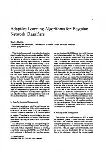
Assuming that x and y are uniformly distributed, we plot a figure in which x any y corresponds to the horizotal and vertical axes respectively, as shown in Figure 1. The shaded area corresponds to the cases in which Equation 5 is true. Since p(E+ |+) > p(E− |+), naive Bayes is optimal in more than a half of the possible area. It is easy to calculate the area of the shaded area, denoted by A. 1 A = − ((p(E+ |+) − p(E− |+)) − 2)2 + 4 2
(6)
It is interesting to notice that, the greater difference between p(E+ |+) and p(E− |+), the greater chance that naive Bayes is optimal. For example, when p(E+ |+) − p(E− |+) = 0.5, the probability of naive Bayes being optimal is 0.78125. Now let us assume that all the dependences among attributes are complete. An attribute Ai is said to depend on Aj completely, if Ai = Aj . If Ai = Aj and all other attributes are independent, the true probablity p(E|+) for an example E = (a1 , a2 , · · · , an ) is Y p(E|+) = p(ai |+) p(ak |+). k6=i,j
The probability pnb (E|+) given by naive Bayes is Y pnb (E|+) = p(ai |+)2 p(ak |+). k6=i,j
10
Harry Zhang and Jiang Su y 1
−1
1
x
y=x+d d
−1
Fig. 1. A figure shows the optimality of naive Bayes in a general case, in which d = p(E− |+) − p(E+ |+), and the shaded area corresponds the optimal area of naive Bayes. + − − + − Given two examples E+ = (a+ 1 , a2 , · · · , an ) and E− = (a1 , a2 , · · · , an ) belonging to the positive and negative class respectively, we have Y Y − p(a− p(a+ p(E+ |+) = p(a+ i |+) k |+). k |+) > p(E− |+) = p(ai |+) k6=i,j
k6=i,j
It is easy to show that, if p(a+ i |+) ≥ 0.5, pnb (E+ |+) > pnb (E− |+). Notice that E+ is a positive example, it is a reasonable assumption that p(a+ i |+) ≥ 0.5. We have a formal definition on the property of such an attribute value. Definition 3. A value ai of attributes Ai is called indicative to class c, if p(Ai = ai |c) ≥ p(Ai = a ¯i |c), where a ¯i is another value of Ai other than ai . For example, for the problem of m-of-n concepts, p(Ai = 1|+) > p(Ai = 0|+) for any attribute. So Ai = 1 is indicative to class +. If all the attribute values of an example are indicative, naive Bayes always gives the optimal ranking for it, illustrated by the theorem below. Theorem 3. Naive Bayes is optimal on example E = (a1 , a2 , · · · , an ) in ranking, if each attribute value of E is indicative to class +. Proof. By induction on i, the number of pairs of attributes with complete dependence. When i = 1, it is true from the preceding discussion. Assume that the claim is true when i = k. That is, if there are k complete dependences among attributes and p(E+ |+) > p(E− |+), then pnb (E+ |+) > pnb (E− |+), where E+ = + − − + − (a+ 1 , a2 , · · · , an ) and E− = (a1 , a2 , · · · , an ) belong to positive and negative class respectively. Consider that i = k + 1. Assume that the new complete dependence is between An−1 and An . Then p(E+ |+) > p(E− |+). Since An−1 = An , + + p(E+ |+) = p(E+ − {An−1 }|+) = p(a+ 1 , · · · , an−2 , an |+), − − p(E− |+) = p(E− − {An−1 }|+) = p(a− 1 , · · · , an−2 , an |+).
Naive Bayesian Classifiers for Ranking
11
Since there are only k dependences among A1 , · · ·, An−2 , An , according to induction hypothesis, + − − + − pnb (a+ 1 , · · · , an−2 , an |+) > pnb (a1 , · · · , an−2 , an |+).
Thus, we have
n Y
p(a+ i |+) >
i=1i6=n−1
n Y
p(a− i |+).
i=1i6=n−1
− Since all the attribute values of E are indicative, p(a+ n−1 |+) > p(an−1 |+). Then, we have n n Y Y p(a+ |+) > p(a− i i |+). i=1
i=1
Therefore, pnb (E+ |+) > pnb (E− |+). Theorem 3 presents a sufficient condition on the local optimality of naive Bayes. Notice that even when all the attribute values of an example are indictative, it is possible that naive Bayes gives a wrong classification.
5
Conclusion
In this paper, we argue that naive Bayes performs well in ranking, just as it does in classification. We compare empirically naive Bayes with the state-ofthe-art decision tree learning algorithm C4.4 in terms of ranking, measured by AUC, and our experiment shows that naive Bayes has some advantage over C4.4. We investigate two example problems theoretically: conjunctive literals and m-of-n concepts, which were used to analyze the classification performance of naive Bayes in [3]. Surprisingly, naive Bayes works perfectly in both problems with respect to ranking, although it does not perform perfectly in terms of classification. For more general cases, we propose a sufficient condition for the local optimality of naive Bayes in ranking. Generally, the performance of naive Bayes in ranking is similar to that in classification, in the sense that both tolerate the estimation error of class probabilities to some extent. It is interesting to know which one tolerates error to a higher extent. Our conjecture is that, for naive Bayes, it might be ranking.
References 1. Bennett, P. N.: Assessing the calibration of Naive Bayes’ posterior estimates. Technical Report No. CMU-CS00-155 (2000) 2. Bradley, A. P.: The use of the area under the ROC curve in the evaluation of machine learning algorithms. Pattern Recognition 30 (1997) 1145-1159 3. Domingos, P., Pazzani M.: Beyond Independence: Conditions for the Optimality of the Simple Bayesian Classifier. Machine Learning 29 (1997) 103-130
12
Harry Zhang and Jiang Su
4. Duda, R. O., Hart, P. E.: Pattern Classification and Scene Analysis. A WileyInterscience Publication (1973) 5. Ferri, C., Flach, P. A., Hernndez-Orallo, J.: Learning Decision Trees Using the Area Under the ROC Curve. Proceedings of the 19th International Conference on Machine Learning. Morgan Kaufmann (2002) 139-146 6. Lachiche, N., Flach, P. A.: Improving Accuracy and Cost of Two-class and Multiclass Probabilistic Classifiers Using ROC Curves. Proceedings of the 20th International conference on Machine Learning. Morgan Kaufmann (2003) 416-423 7. Frank, E., Trigg, L., Holmes, G., Witten, I. H.: Naive Bayes for Regression. Machine Learning 41(1) (2000) 5-15 8. Friedman, N., Greiger, D., Goldszmidt, M.: Bayesian Network Classifiers. Machine Learning 29 (1997) 103–130 9. Hand, D. J., Till, R. J.: A simple generalisation of the area under the ROC curve for multiple class classification problems. Machine Learning 45 (2001) 171-186 10. Kononenko, I.: Comparison of Inductive and Naive Bayesian Learning Approaches to Automatic Knowledge Acquisition. Current Trends in Knowledge Acquisition. IOS Press (1990) 11. Ling, C. X., Huang, J., Zhang, H.: AUC: a statistically consistent and more discriminating measure than accuracy. Proceedings of the International Joint Conference on Artificial Intelligence IJCAI03. Morgan Kaufmann (2003) 329-341 12. Ling, C. X., Yan, R. J.: Decision Tree with Better Ranking. Proceedings of the 20th International Conference on Machine Learning. Morgan Kaufmann (2003) 480-487 13. Merz, C., Murphy, P., Aha, D.: UCI repository of machine learning databases. Dept of ICS, University of California, Irvine (1997). http://www.ics.uci.edu/ mlearn/MLRepository.html 14. M. Pazzani, P., Merz, C., Murphy, P., Ali, K., Hume, T., Brunk, C.: Reducing misclassification costs. Proceedings of the 11th International conference on Machine Learning. Morgan Kaufmann (1994) 217-225 15. Provost, F., Fawcett, T.: Analysis and visualization of classifier performance: comparison under imprecise class and cost distribution. Proceedings of the Third International Conference on Knowledge Discovery and Data Mining. AAAI Press (1997) 43-48 16. Provost, F., Fawcett, T., Kohavi, R.: The case against accuracy estimation for comparing induction algorithms. Proceedings of the Fifteenth International Conference on Machine Learning. Morgan Kaufmann (1998) 445-453 17. Provost, F. J., Domingos, P.: Tree Induction for Probability-Based Ranking. Machine Learning 52(3) (2003) 199-215 18. Swets, J.: Measuring the accuracy of diagnostic systems. Science 240 (1988) 12851293 19. Zadrozny, B., Elkan, C.: Obtaining calibrated probability estimates from decision trees and naive Bayesian classifiers. Proceedings of the Eighteenth International conference on Machine Learning. Morgan Kaufmann (2001) 609-616 20. Witten, I. H., Frank, E.: Data Mining –Practical Machine Learning Tools and Techniques with Java Implementation. Morgan Kaufmann (2000)