IEEE ANTENNAS AND WIRELESS PROPAGATION LETTERS, VOL. 9, 2010
649
Local High-Resolution Technique in FDTD Modeling of ELF Propagation in the Earth–Ionosphere Cavity Hangang Xia, Yi Wang, and Qunsheng Cao
Abstract—In this letter, a local high-resolution technique (LHRT) of three-dimensional finite-difference time-domain (3D-FDTD) method is presented for the extremely low-frequency (ELF) electromagnetic (EM) wave propagation in the Earth–ionosphere cavity. This new model is useful for the analysis of the ELF EM wave propagating in a specific region, where the required space interval of the grid-cell is extremely fine. Once the length of the required space interval in the specific region and the cutoff frequency of the source are determined, the model of Earth–ionosphere cavity can be established automatically. It is verified that the simulation results of the new technique are as accurate as those of the traditional methods. Index Terms—Extremely low-frequency (ELF), finite-difference time-domain (FDTD) method, local high-resolution technique (LHRT).
I. INTRODUCTION BSERVATIONS of electromagnetic (EM) signals in the frequency range 3–300 Hz have become a potential tool for a variety of applications such as remote sensing, underwater communication, and earthquake prediction. The techniques available in the literature for the study of extremely low-frequency (ELF) propagation before 2000 were primarily based upon frequency-domain waveguide theory [1]. Later, time-domain techniques became more popular and enhanced more capability. In 2002–2004, Simpson and Taflove proposed a technique for merging adjacent cells in the east–west direction as either pole is approached for improving numerical efficiency [2], [3]. Soriano et al. [4], Otsuyama et al. [5], Yang et al. [6], and Wang et al. [7] had utilized ELF EM wave propagation based on Holland’s spherical finite-difference time-domain (FDTD) method [8]. Simulated results, in a certain local region (e.g., a country), named as “specific regions” where the resolution of the FDTD mesh needs to be as high as possible, are more preferable than those in other regions. A new algorithm using local high-resolution technique (LHRT) is proposed to cater this requirement. The mesh of Earth–ionosphere cavity constructed by LHRT is plotted in Figs. 1 and 2(a), and the grid-cells selected from the
O
Manuscript received April 01, 2010; revised May 09, 2010 and June 09, 2010; accepted June 10, 2010. Date of publication June 21, 2010; date of current version July 19, 2010. This work was supported by the Natural Science Foundation of Jiangsu Province under Grant BK2009368 (China). The authors are with the College of Information Science and Technology, Nanjing University of Aeronautics and Astronautics, Nanjing 210016, China (e-mail:
[email protected];
[email protected];
[email protected]). Color versions of one or more of the figures in this letter are available online at http://ieeexplore.ieee.org. Digital Object Identifier 10.1109/LAWP.2010.2053343
Fig. 1. FDTD modeling of Earth-ionosphere cavity using local high-resolution technique (LHRT).
Fig. 2. (a) Mesh of Earth–ionosphere cavity viewed from the North Pole, the lower fan-shaped frame zone of which is the specific region. (b) Grid-cells selected from the upper fan-shaped frame zone of (a).
upper fan-shaped frame zone of Fig. 2(a) are enlarged to be plotted in Fig. 2(b). LHRT is helpful to achieve high resolution in a specific region without increasing computational memory dramatically. Unlike Simpson and Taflove [2], [3], here the number of FDTD cells in the east–west direction does not change with latitude. Simpson and Taflove deal with the issue of grid cells in a standard latitude–longitude spherical grid that gets very small upon approaching the North and South poles, and time-step is reduced greatly by the merging cell technique. LHRT is for finer spatial resolution in a local region. These two techniques are complementary. Besides, LHRT is different from subgridding technique. Upgrading the resolution level in a localized region certainly leads to the change of the grid-cell sizes along
1536-1225/$26.00 © 2010 IEEE
650
IEEE ANTENNAS AND WIRELESS PROPAGATION LETTERS, VOL. 9, 2010
TABLE I SETTINGS FOR THE FDTD SIMULATIONS (IDEAL)
TABLE II DETAILS OF THE MESH FOR EACH IDEAL EXPERIMENT
According to the numerical stability condition [9], stricted by the 3-dB cutoff frequency of the source
is re-
(5) where is the speed of light in vacuum. and can be determined by (3)–(5). Then, with the help of Fig. 2(b), we obtain an entire Great Circle in the – directions (not just a localized region), as it shown in Fig. 1. (6) II. MODEL FORMULATION Earth–ionosphere cavity is almost spherically symmetrical, so the spherical coordinate system is suitable for its modeling. First, divide the Earth’s spherical surface by a number of longitude and latitude lines shown in Fig. 2(a). In [2], the radians between each longitude line (or latitude line) are defined as one ). However, the radians in LHRT are treated as two value ( and ), as they are labeled in Fig. 2(a). For lonvalues ( gitude (or latitude), and are defined in the specific region and the rest of regions, respectively. Under the definition of spherical coordinate ( - - system) and the assumption of and , we can obtain
in specific region in the rest of region in specific region in the rest of region is determined by the space interval specific region on the ground. We write
(1)
(7) and are defined as the numbers of cells in - and -directions, respectively. Then, the closed spherical surface can be cells, the shapes of which are approxidivided into mately treated as isosceles-trapezoidal or isosceles-triangular, as shown in Fig. 2(a). The computational space is divided into segments in -direction, so Earth–ionosphere cavity is dicells. vided into Consider defined in Fig. 2(b) and apply the Ampere’s Law in integral form mentioned in [9], and we have
(2)
required in the
(3) (8) where is the radius of the Earth and is marked in Fig. 2(b). is determined by the space interval , which is defined as the space interval in the rest of regions on the ground as labeled in Fig. 2(b). We have
is the area of isosceles-trapezoidal labeled where in Fig. 2(b). As the resolution is sufficiently high, we write
(4)
(9)
XIA et al.: LOCAL HIGH-RESOLUTION TECHNIQUE IN FDTD MODELING OF ELF PROPAGATION IN EARTH–IONOSPHERE CAVITY
651
Fig. 3. Waveform of E ; 3-dB cutoff frequency of the source is 10 Hz. Fig. 5. Waveform of E at the 3-dB cutoff frequency of 10 Hz at the equator.
Fig. 4. Waveform of E ; 3-dB cutoff frequency of the source is 100 Hz.
Similarly, the updated equations of
can be derived Fig. 6. Waveform of E at the 3-dB cutoff frequency of 100 Hz at the equator.
(10) The updated equations in the poles where the shape of the cell is isosceles-triangular are not present, as their formats are is restricted by the similar to those in [2]–[7]. Time-step minimum of and
(11) With the help of (10)–(11) and other EM components’ updated equations we have not listed, the modeling of Earth–ionosphere cavity can be established completely. III. RESULTS AND DISCUSSIONS Two ideal experiments are presented in this section, the settings and details of which are listed in Tables I and II. From
Table II, it is obvious that with the frequency shifting from 100 to 10 Hz, the total number of cells required in the FDTD simulation is reduced sharply. LHRT is more efficient for applications in which the required frequency is as low as possible. at the observation station are plotted Time-waveforms of in Figs. 3 and 4. In Fig. 3, the pulse duration ( ) of the EM wave is 0.2 s; however, traveling around the whole world needs only 0.134 s. This causes aberration of the waveform. In Fig. 4, the pulse duration is only 0.02 s, which is much smaller than the circumglobal traveling time. Thus, the waveform will not be at the same observachanged largely. Time-waveforms of tion without LHRT are also plotted. Actually, for the traditional method, it is difficult to obtain the value of an EM field at the point only 1 km away from the source directly. In this letter, the results marked with dotted lines are obtained by linearly interfield quantities at the neighboring grids. In order polating the to limit the error brought by the linear interpolation, the resolution of the whole Earth needs to be as high as possible. In the present experiments, the numbers of total cells are chosen as 200 100 52 (for 10 Hz) and 500 250 52 (for 100 Hz). As they are shown in Figs. 3 and 4, the deviations between the
652
IEEE ANTENNAS AND WIRELESS PROPAGATION LETTERS, VOL. 9, 2010
IV. CONCLUSION In this letter, we put forward the local high-resolution technique used in the 3D-FDTD modeling of the ELF EM wave propagation in Earth–ionosphere cavity scheme, in which the space interval is reduced with sufficient flexibility to meet the requirements of practical measurement. The results of our new method agree well with those of the mature models and reduce large quantities of memory consumption. This model is useful for the practical measurement of the ELF EM fields in specific regions and for other special applications.
REFERENCES Fig. 7. Color-map of information.
E
on the ground under the influence of geographic
results of the traditional method and LHRT are small, no more than 3%. That is the indication that LHRT is accurate enough for use. On the other hand, for the traditional method, good accuracy (compared to LHRT) comes at the expense of huge memory and time consumption. at the equator are plotted in Figs. 5 Space waveforms of and 6. When the frequency is chosen as 10 Hz in Fig. 5, the EM wave is almost a standing wave, as it was stated in [10]. The wave nodes are located at 0 and 180 E (W), and the wave loops are located at 90 E and 90 W. When the frequency is changed to 100 Hz, the EM wave becomes a traveling wave, as it is shown in Fig. 6. The EM wave always has phase reversal illustrated in Fig. 4 and gathers at the antipode of the source (90 W) shown in Fig. 6. The space waveforms at the equator fit the theory stated in [10] and [11]. In the following nonideal experiment, China is the “specific region.” A “knee” altitude profile of conductivity from [12] is applied for the ionosphere. For the lithosphere, conductivities are assigned according to [13]. A unit horizontal dipole is placed on the ground at the at Wenchuan, China. The color-map of propagation time 0.034 s is surfaced in Fig. 7. It is illustrated that the propagation of the EM wave is fully influenced by different geometrical structures and media of the Earth. A potential application for our software with LHRT embedded would be to simulate and study the ELF EM anomaly in the Wenchuan earthquake that occurred on May 12, 2008.
[1] L. Sevgi, F. Akleman, and L. B. Felsen, “Groundwave propagation modeling: Problem-matched analytical formulations and direct numerical techniques,” IEEE Antennas Propag. Mag., vol. 44, no. 1, pp. 55–75, Feb. 2002. [2] J. J. Simpson and A. Taflove, “Two-dimensional FDTD model of antipodal ELF propagation and Schumann resonances of the earth,” IEEE Antennas Wireless Propag. Lett., vol. 1, pp. 53–56, 2002. [3] J. J. Simpson and A. Taflove, “Three-dimensional FDTD modeling of impulsive ELF propagation about the earth-sphere,” IEEE Trans. Antennas Propag., vol. 52, no. 2, pp. 443–451, Feb. 2004. [4] A. Soriano et al., “Finite difference time domain simulation of the Earth-ionosphere resonant cavity: Schumann resonances,” IEEE Trans. Antennas Propag., vol. 53, no. 4, pp. 1535–1541, Apr. 2005. [5] T. Otsuyama, D. Sakuma, and M. Hayakawa, “FDTD analysis of Schumann resonances for realistic subionospheric waveguide models,” in Proc. IEE Japan, 2003, vol. EMT-03, pp. 21–24. [6] H. Yang and V. P. Pasko, “Three-dimensional finite difference time domain modeling of the Earth-ionosphere cavity resonances,” Geophys. Res. Lett., vol. 32, pp. L03114-1–L03114-4, 2005. [7] Y. Wang, H. Xia, and Q. Cao, “Analysis of ELF propagation along the earth surface using the FDTD model based on the spherical triangle meshing,” IEEE Antennas Wireless Propag. Lett., vol. 8, pp. 1107–1020, 2009. [8] R. Holland, “THREDS: A finite-difference time-domain EMP code in3-D spherical coordinates,” IEEE Trans. Nucl. Sci., vol. NS-30, no. 6, pp. 4592–4595, Dec. 1983. [9] A. Taflove and S. C. Hagness, Computational Electrodynamics: The Finite Difference Time-Domain Method, 3rd ed. Norwood, MA: Artech House, 2005. [10] P. Bannister, “ELF propagation update,” IEEE J. Ocean. Eng., vol. OE-9, no. 3, pp. 179–188, Jul. 1984. [11] J. Galejs, Terrestrial Propagation of Long Electromagnetic Wave. New York: Pergamon, 1972. [12] C. Greifinger and P. Greifinger, “Approximate method for determining ELF eigenvalues in the earth-ionosphere cavity,” Radio Sci., no. 13, p. 831, 1978. [13] J. Hermance, “Electrical conductivity of the crust and mantle,” in Global Earth Physics: A Handbook of Physical Constants. Washington, DC: AGU, 1995, pp. 190–205.