LOCAL LINEARIZATION METHOD FOR NUMERICAL INTEGRATION ...

LOCAL LINEARIZATION METHOD FOR NUMERICAL INTEGRATION OF DELAY DIFFERENTIAL EQUATIONS∗ J.C. JIMENEZ, L. M. PEDROSO, F. CARBONELL

AND V. HERNANDEZ †

Abstract. In this paper, a new approach for the numerical computation of Delay Differential Equations (DDEs) is introduced. The essential idea consists on obtaining numerical integrators that use a code expressly developed for linear DDEs, in contrast with the conventional approach of using a code for ordinary differential equations. Specifically, two numerical schemes of such new class of integrators are proposed and their numerical viability is analyzed. It includes the estimation of the convergence rate, the evaluation of the computational cost of the schemes and a simulation study. It is proved that, these one-step explicit integrators converge uniformly with order two to the solution of nonlinear DDEs and they are able to integrate stiff equations in a satisfactory way with low computational cost. Key words. delay differential equations, local linearization methods, numerical integrators AMS subject classifications. 34K28, 65L05, 65L20

1. Introduction. In recent years the interest in the numerical solution of Delay Differential Equations (DDEs) with constant delay has been increased. It has been motivated by their applicability in the mathematical modelling of several physical, chemical and biological processes, where they provide the best and sometimes the only realistic simulation of the observable phenomena [7, 17, 30]. There exist a variety of such numerical integrators, which essentially have two main ingredients [2]: 1) the emulation of the method of the steps in order to obtain piecewise Ordinary Differential Equations (ODEs); and 2) the application of a variable step-size ODE code with a suitable approximation of the retarded solutions. Examples are the schemes proposed in the papers [8, 21, 23, 25, 27, 33, 34, 41], which use several ODE codes (e.g., Euler, Runge-Kutta, multi-steps and Local Linearization) and several ways to approximate the retarded solutions (e.g., polynomial functions, θ-methods, continuous extensions of Runge-Kutta and Local Linearization methods). Although the convergence and linear stability of these methods have been well studied, it is not the case of the preserving qualitative features of such methods [2]. It is well known [13, 39] that, in general, the conventional numerical integrators for ODEs do not preserve the dynamical properties of the original ODEs. Therefore, it is expected that the numerical integrators for DDEs derived from the above mentioned ODE codes neither preserve the dynamic properties of the original DDEs. It is also well known that for the stability analysis of ODEs, as well as for DDEs, there are two main techniques [2]: 1) the Lyapunov theory and 2) the stability theory in first approximation. The latter, the simpler one, is based on the local linearization of the differential equations. This kind of linearization is also the main component of the so called Local Linearization (LL) integrators for ODEs. In recent papers [26, 15], it has been shown that this type of schemes preserve the dynamical properties of the original equations much better than the conventional numerical integrators. For intance, under quite general conditions, they have not spurious equilibrium points and preserve the local stability of the exact solution at hyperbolic equilibrium points ∗ This work was partially supported by the Research Grant 03-059 RG/MATHS/LA from the Third World Academy of Science. † Instituto de Cibern´ etica Matem´ atica y F´ısisca, Calle 15 No. 551 entre C y D, Vedado, La Habana 10400, Cuba([email protected]).

1

2

J.C. JIMENEZ, L. M. PEDROSO, F. CARBONELL V. HERNANDEZ

and periodic orbits. On the other hand, this linealization approach has been the key for the construction of efficient and stable numerical schemes for the integration and estimation of various classes of random dynamical systems (see [28, 29, 36, 37] and references therein). Specifically, in the framework stochastic and random differential equations, simulations studies have shown that the LL integrators have similar stability properties than the conventional implicit integrators with the computational efficiency of the explicit ones (see for instance [5, 10, 9]). In addition, in the framework of the nonlinear filtering problems the LL filters have similar features (see for instance [35]). In all the cases, the piecewise linealization of the vector fields that define the differential equations to be integrated is the keystone in the construction of the LL integrators and, at the same time, the main difference with the conventional numerical integrators (which are typically derived from a primary expansion of the unknown solution in power series). Thus, the application of this Local Linealization approach for the integration of DDEs is also attractive. The goal of this paper is studying the numerical viability of the Local Linearization approach for defining a new type of numerical integrators for DDEs, leaving the qualitative analysis of them for a further paper. The essential ideas of this approach are: 1) approximate linearly the vector field of the DDE in order to obtain a piecewise linear DDE, and 2) compute the solution of such linear equations by the variation of constant formula with a suitable approximation of the retarded solutions. The paper is organized as follow. In section 2, the LL method is introduced and two numerical schemes are proposed. In section 3, the convergence of the method is studied, while in the last section a simulation study is carried out in order to illustrate the performance of the method. 2. Local linearization method. Let f : R × Rm × Rm −→ Rm be a differentiable function and let x(t) be the solution of the m-dimensional DDE dx (t) = f (t, x (t) , xt (−τ )) , t ∈ [t0 , T ] , dt xt0 (s) = ϕ (s) , s ∈ [−τ, 0]

(2.1) (2.2)

at the point t ∈ [t0 − τ, T ], where τ > 0 is a constant delay, ϕ : [−τ, 0] −→ Rm is a given initial function, and xt : [−τ, 0] −→ Rm is the segment function defined as xt (s) := x(t + s), s ∈ [−τ, 0] , for all t ∈ [t0 , T ]. Lipschitz and smoothness conditions on the function f are also assumed in order to ensure an unique solution for the equation (2.1)-(2.2). Let (t)h = {t0 < t1 < ... < tn < ... ≤ T } be a partition of the time interval [t0 , T ] such that sup(tn+1 − tn ) ≤ h < 1, n

(2.3)

and define nt := max{n = 0, 1, 2, ..., : tn ≤ t and tn ∈ (t)h }, for t ∈ [t0 , T ]. Throughout this paper it will be assumed that condition h < τ holds. Suppose that, for all tn ∈ (t)h , yn ∈ Rm is a point close to x (tn ). For all et : [−τ, 0] −→ Rm be a segment function that approximate to xt , such t ∈ [t0 , T ], let y etn (0) = yn for all tn ∈ (t)h . that y

3

LOCAL LINEARIZATION METHOD FOR DDES

In addition, let us consider the first order Taylor expansion of the function f etn (−τ )), around the point (tn , yn , y etn (−τ )) + fx (tn , yn , y etn (−τ ))(u − yn ) f (s, u, v) ≈ f (tn , yn , y etn (−τ ))(v − y etn (−τ )) + ft (tn , yn , y etn (−τ ))(s − tn ), +fxt (tn , yn , y for s ∈ R and u, v ∈ Rm , where fx , fxt and ft denote the partial derivatives of f with respect to the variables x, xt and t, respectively. Taking into account that f can be linearly approximated by its first order Taylor expansion, the solution of (2.1)-(2.2) can be locally approximated on each interval [tn , tn+1 ) by the solution of the linear DDE dz (t) etn (−τ ), t ∈ [tn , tn+1 ) = An z(t) + Bn zt (−τ ) + cn t − cn tn + dn − An yn − Bn y dt etn (s), s ∈ [−τ, 0] ztn (s) = y (2.4) which is given by [20] t−t Z n

z(t) = e

An (t−tn )

etn (−τ )) + cn u + dn e−An u (Bn (e ytn (u − τ ) − y

{yn + 0

−An yn )du},

(2.5)

etn (−τ )), Bn = fxt (tn , yn , y etn (−τ )) are constant matrices, where An = fx (tn , yn , y etn (−τ )), dn = f (tn , yn , y etn (−τ )) are constant vectors and tn , tn+1 ∈ cn = ft (tn , yn , y (t)h . Further, by using the identity Z∆ exp(−An u)du An = −(exp(−An ∆) − I),

∆≥0

(2.6)

0

and simple rules from the integral calculus, the above expression can be conveniently rewritten as etn ), z(t) = yn + Φ(tn , yn , t − tn ; y

(2.7)

where t−t Z n

etn (−τ )) + dn )du eAn (t−tn −u) (Bn (e ytn (u − τ ) − y

e tn ) = Φ(tn , yn , t − tn ; y 0

t−t Z nZu

eAn (t−tn −u) cn drdu.

+ 0

(2.8)

0

In this way, by setting y0 = x(t0 ) and iterativelly evaluating the expression (2.7) at tn+1 (for n = 0, 1...) a sequence of points e tn ) yn+1 = yn + Φ(tn , yn , tn+1 − tn ; y can be obtained as an approximation to the solution x of (2.1)-(2.2) at each point tn+1 ∈ (t)h . This just defines the Local Linear discretization of a DDE. More precisely:

4

J.C. JIMENEZ, L. M. PEDROSO, F. CARBONELL V. HERNANDEZ

Definition 2.1. For a time discretization (t)h , the Local Linear Discretization of the solution of (2.1)-(2.2) at each point tn+1 ∈ (t)h is defined by the recursive expression e tn ) yn+1 = yn + Φ(tn , yn , tn+1 − tn ; y

(2.9)

etn : [−τ, 0] −→ Rm is a segment function that approximate to xtn , such that where y etn (0) = yn . y Moreover, an approximation for x in the whole interval [t0 − τ, T ] is stated in the definition below. Definition 2.2. For a time discretization (t)h , the Local Linear Approximation of the solution of (2.1)-(2.2) is defined by the function etnt ), y (t) = ynt + Φ(tnt , ynt , t − tnt ; y

(2.10)

for all t ∈ [t0 , T ], and by y (t) = ϕ (t) , etnt is for t ∈ [t0 − τ, t0 ]. Here, ynt denotes the LL discretization (2.9) at nt , and y the segment function of Definition 2.1. In addition, for t ∈ [t0 , T ], let yt : [−τ, 0] −→ Rm be the segment function defined as yt (s) := y(t + s), s ∈ [−τ, 0] , where y(t + s) is the LL Approximation (2.10) evaluated at the point t + s. It is clear that the LL Approximation is a continuous function that coincides with the LL Discretization at each point of the time discretization (t)h . As it can be noted from the definition, to compute the Local Linear Discretization etn to xtn is assumed to be given. Based at the time tn+1 an suitable approximation y on the choice of such approximation, different kind of LL schemes could be defined. In the next subsections, two LL schemes will be introduced. 2.1. Natural LL scheme. Let consider the numerical scheme that is defined in et (s) as the LL Approximation yt (s) for all s ∈ [−τ, 0] and a natural way by taking y t + s ∈ [t0 , T ]. Specifically, the scheme shall be defined through the expression (2.9) etn ≡ ytn for all tn ∈ (t)h \t0 , and y et0 (s) ≡ ϕ(s), with y e for all s ∈ [−τ, 0], where ϕ e is an approximation to ϕ that shall be defined bellow. In this subsection, and only here, it is assumed that the points in the time discretization (t)h are equidistants, i.e., tn+1 − tn = h = Nτ0 , for a fixed N0 ∈ N+ . Consider the times tn , n = 0, ..., N0 for which t0 ≤ tn ≤ t0 + τ , and denote sn = tn − τ . Suppose that, in the interval [sn , sn+1 ], the initial function ϕ in (2.2) can be exponentially approximated by the function ϕ e (sn + u) = ϕ (sn ) + LeTn u R, u ∈ [0, h] ,

(2.11)

where Tn , L and R are certain constant matrices such that LeTn u R ∈ Rm . For p P instance, when ϕ(sn + u) is approximated by the interpolating polynomial αi,n ui i=0

5

LOCAL LINEARIZATION METHOD FOR DDES

these matrices can be chosen as  0m×m p!αp,n (p − 1)!αp−1,n  0 0 1    0 0 0 Tn =   . . .. ..  .. .   0 0 ··· 0 0 ···

··· ··· .. . ..

 α1,n 0   ..  .   ∈ R(m+p)×(m+p) ,  0   1  0

2α2,n 0 .. .

.

1 0 0

0 0

L = (Im , 0m×p ) and R| = (01×m+p−1 , 1), where the coefficients αi,n are obtained from interpolating conditions. The statement above is straightforwardly derived from Lemma 6.1 in Appendix and the expression p X

Zu i

αi,n u = α0,n +

i=0

α1,n ds +

p X

i!αi,n

i=2

0

sZi−1

Zu Zs1 ... 0

0

dsi dsi−1 ...ds1 ,

(2.12)

0

with α0,n = ϕ (sn ). etn (u − τ ) = ϕ Taking into account that y e (sn + u) it is follows that Zh e tn ) = Φ(tn , yn , h; y

Zh Zu e

An (h−u)

(Bn Le

Tn u

eAn (h−u) cn drdu,

R + dn )du +

0

0

0

which, by (2.6), can be rewritten as Zh

Zh Zu

eAn (h−u) Bn LRdu

eAn (h−u) Bn LeTn r Tn Rdrdu +

e tn ) = Φ(tn , yn , h; y 0

0

0

Zh

Zh Zu eAn (h−u) dn du +

+ 0

eAn (h−u) cn drdu. 0

0

Now, since LR = 0m×1 , by Lemma 6.1 it is obtained that etn ) = L0 eT0,n h R0 , Φ(tn , yn , h; y where



T0,n

An  0  = 0 0

Bn L Tn 0 0

cn 0 0 0

 dn Tn R   , tn ∈ [t0 , t0 + τ ],  1 0

L0 = (Im , 0m×m+p+2 ) and R|0 = (01×2m+p+1 , 1). Therefore, for t0 ≤ tn ≤ t0 + τ , the expression yn+1 = yn + L0 eT0,n h R0 , n = 0, ..., N0 − 1, defines a Local Lineal Discretization, while the expression y (t) = ynt + L0 eT0,n (t−tnt ) R0 , n = 0, ..., N0 − 1,

(2.13)

6

J.C. JIMENEZ, L. M. PEDROSO, F. CARBONELL V. HERNANDEZ

defines a Local Linear Approximation for all t ∈ [t0 , t0 + τ ]. Taking into account the analogy between the expressions (2.13) and (2.11), the procedure above can be used to extend the LL Approximation to t0 +τ ≤ tn ≤ t0 +2τ , and so on. In this way, for t0 + kτ ≤ tn ≤ t0 + (k + 1) τ with k = 1, 2, ..., it is obtained the expression yn+1 = yn + Lk eTk,n h Rk , n = kN0 , ..., (k + 1)N0 − 1, which defines the natural LL scheme. Here, the matrices Tk,n , Lk and Rk are recursively defined by 

Tk,n

An  0 =  0 0

Bn Lk−1 Tk−1,n 0 0

cn 0 0 0



dn

Tk−1,n Rk−1   , tn ∈ [t0 + kτ, t0 + (k + 1)τ ].  1 0

Lk = (Lk−1 , 0m+2 ) and R|k = (01×m+2 , R|k−1 ). Note that the natural LL scheme produces the exact solution of linear DDEs with polynomial or exponential initial condition. Thus, obviously, the numerical solution provided by it preserves the stability properties of linear DDEs. However, observe also that the dimension of the matrices Tk,n increase with k, which increse the computational cost of the scheme when τ 0, i=1,··· ,d

i = 1, · · · , d, are constant delays. xt is a segment function defined as at the begining of Section 2. By following the same ideas of the previous subsections, the definitions of the LL Discretization and LL Approximation are easily extended to equations with multiple delays. In this case, the expressions (2.9) and (2.10) are also obtained but with Φ defined by the form Zhn et1n , .., y etdn ) Φ(tn , yn , hn ; y

=

d X etin (−τi )) + dn )du eAn (hn −u) ( Bin (e ytin (u − τi ) − y i=1

0

ZhnZu eAn (hn −u) cn drdu.

+ 0

0

(2.16)

8

J.C. JIMENEZ, L. M. PEDROSO, F. CARBONELL V. HERNANDEZ

etin : [−τi , 0] −→ Rm is the segment function defined by where y etin (s) := y e i (tn + s), s ∈ [−τi , 0] , y e i : [tn − τi , tn ] −→ Rm is a suitable approximation to x(t) for all t ∈ [tn − τi , tn ] and y e i (tn ) = yn . In expression (2.16), tn , tn+1 ∈ (t)h , hn = tn+1 − tn , such that y et1n (−τ1 ), ..., y etdn (−τd )), Bin = fxt (−τi ) (tn , yn , y et1n (−τ1 ), ..., y etdn (−τd )) An = fx (tn , yn , y are constant matrices and etdn (−τd )) and dn = f (tn , yn , y et1n (−τ1 ), ..., y etdn (−τd )) et1n (−τ1 ), ..., y cn = ft (tn , yn , y are constant vectors. ft , fx and fxt (−τi ) denote, respectively, the partial derivatives of f with respect to the variables t, x and xt (−τi ). In this way, the LL schemes proposed in the subsections above are easily extended to DDEs with multiple delays. 3. Convergence Analysis. For sake of simplicity, in this section it is assumed that there is a single delay. Suppose also that the initial function ϕ in (2.2) satisfies the boundedness and Lipschitz conditions sup kϕ(s)k ≤ M0

(3.1)

−τ ≤s≤0

and kϕ(s2 ) − ϕ(s1 )k ≤ M1 (s2 − s1 ),

(3.2)

for −τ ≤ s1 ≤ s2 ≤ 0; and the function f in (2.1) and its first partial derivatives satisfice the following Lipschitz conditions kf (t, u1 , v1 ) − f (t, u2 , v2 )k≤λ0 (ku1 − u2 k + kv1 − v2 k), kfx (t, u1 , v1 ) − fx (t, u2 , v2 )k≤λ1 (ku1 − u2 k + kv1 − v2 k), kfxt (t, u1 , v1 ) − fxt (t, u2 , v2 )k≤λ2 (ku1 − u2 k + kv1 − v2 k), kft (t, u1 , v1 ) − ft (t, u2 , v2 )k≤λ3 (ku1 − u2 k + kv1 − v2 k),

(3.3) (3.4) (3.5) (3.6)

for all u1 , u2 , v1 , v2 ∈ Rm , t ∈ R. Further, suppose that f and its first and second partial derivatives satisfice the linear growth and boundedness conditions kf (t, u, v)k + kft (t, u, v)k ≤ K0 (1 + kuk + kvk), kfx (t, u, v)k + kfxt (t, u, v)k ≤ K1 ,

(3.7) (3.8)

and kfxx (t, u, v)k + kfxxt (t, u, v)k + kfxt xt (t, u, v)k + kftt (t, u, v)k + kftx (t, u, v)k + kftxt (t, u, v)k ≤ K2 for all u, v ∈ Rm , t ∈ R.

(3.9)

9

LOCAL LINEARIZATION METHOD FOR DDES

3.1. Local truncation error. In this subsection, the local trucation error of the LL Discretization shall be derived. With that proposal the next two lemmas shall be used. The first one establishes an uniform bound and Lipschitz condition for the solution of the DDE, whereas the second one states a Lipschitz-type condition for the function Φ with respect to its second and fourth arguments. Lemma 3.1. Assuming that conditions (3.1), (3.2) and (3.7) hold, there exist positive constants C0 and C1 such that sup t0 −τ ≤t≤T

kx(t)k ≤ C0

(3.10)

and kx(s2 ) − x(s1 )k ≤ C1 (s2 − s1 )

(3.11)

hold for t0 − τ ≤ s1 ≤ s2 ≤ T , where x is the solution of the equation (2.1)-(2.2). Proof. From the integral form of the equation (2.1)-(2.2) follows that Zt kx(t)k ≤ kϕ(0)k +

kf (s, x (s) , xs (−τ ))k ds, t ≥ t0 t0

which by conditions (3.1) and (3.7) leads to Zt kx(t)k ≤ M0 +

K0 (1 + kx (s)k + kxs (−τ )k)ds. t0

Hence Zt sup t0 −τ ≤u≤t

kx(u)k ≤ M0 +

K0 (1 + 2 t0

sup

kx(u)k)ds,

t0 −τ ≤u≤s

and (3.10) follows from the Gronwall inequality. On the other hand, for t0 − τ ≤ s1 ≤ s2 ≤ t0 the inequality (3.11) follows from condition (3.2). Whereas, for t0 ≤ s1 ≤ s2 ≤ T it is obtained Zs2 kx(s2 ) − x(s1 )k ≤

kf (s, x (s) , xs (−τ ))k ds s1

≤ (s2 − s1 )K0 (1 +

sup (kx (s)k + kxs (−τ )k)),

s1 ≤s≤s2

which by (3.10) gives kx(s2 ) − x(s1 )k ≤ K0 (1 + 2C0 )(s2 − s1 ), and so the proof concludes. Lemma 3.2. Let tn , tn+1 ∈ (t)h and hn = tn+1 − tn . Under the conditions (3.1)-(3.8), there exists a positive constant P such that kΦ(tn , v, hn ; ztn ) − Φ (tn , x (tn ) , hn ; xtn )k ≤ hn P (kv − x(tn )k + sup kztn (s − τ ) − xtn (s − τ )k) s∈[0,hn ]

10

J.C. JIMENEZ, L. M. PEDROSO, F. CARBONELL V. HERNANDEZ

where x is the solution of (2.1)-(2.2), Φ is defined as in (2.8), v ∈ Rm , ztn : [−τ, 0] −→ Rm is a segment function defined as ztn (s) := z(tn + s), s ∈ [−τ, 0] , and z : [tn − τ, tn ] −→ Rm is a function. Proof. Define Rn := Φ(tn , v, hn ; ztn ) − Φ (tn , x (tn ) , hn ; xtn ) , which in turn can be written as Zhn eAn (hn −u) (Bn (ztn (u − τ ) − ztn (−τ )) + ucn + dn )du

Rn = 0

Zhn eAn (hn −u) (Bn (xtn (u − τ ) − xtn (−τ )) + ucn + dn )du,

− 0

where An = fx (tn , v, ztn (−τ )), Bn = fxt (tn , v, ztn (−τ )), An = fx (tn , x (tn ) , xtn (−τ )), Bn = fxt (tn , x (tn ) , xtn (−τ )) are constant matrices and cn = ft (tn , v, ztn (−τ )) , dn = f (tn , v, ztn (−τ )), cn = ft (tn , x (tn ) , xtn (−τ )) , dn = f (tn , x (tn ) , xtn (−τ )) are constant vectors. By using Lemma 6.3 in Appendix it is obtained that Zhn° ° ° ° ° ° ° ° kRn k ≤ °eAn (hn −u) − eAn (hn −u) ° (°Bn ° kxtn (u − τ ) − xtn (−τ )k + u kcn k + °dn °)du 0

+

Zhn° ° ° ° ° ° An (hn −u) ° ° °e ° (°Bn ztn (−τ ) − Bn xtn (−τ )° + u kcn − cn k + °dn − dn ° 0

° ° + °Bn ztn (u − τ ) − Bn xtn (u − τ )°)du. From the Finite Increments Inequality, conditions (3.8), (3.4) and constraint (2.3) it is follows that ° ° ° ° ° An (hn −u) ° − eAn (hn −u) ° ≤ eK1 hn hn °An − An ° °e ≤ eK1 λ1 hn Γn , where Γn = kv − x(tn )k + sup kztn (u − τ ) − xtn (u − τ )k . u∈[0,hn ]

In addition, from Lemmas 6.3 and 3.1, and conditions (3.5) and (3.8) it is follows that ° ° °Bn zt (u − τ ) − Bn xtn (u − τ )° ≤ kBn k kztn (u − τ ) − xtn (u − τ )k n ° ° + °Bn − Bn ° kxt (u − τ )k n

≤ (K1 + λ2 C0 ) Γn

LOCAL LINEARIZATION METHOD FOR DDES

11

for all u ∈ [0, hn ]. By using the two previous inequalities, Lemma 3.1, and conditions (3.3), (3.6), (3.7) and (3.8) it is obtained that Zhn eK1 λ1 hn (2K1 C0 + K0 (1 + 2C0 )u + K0 (1 + 2C0 ))du

kRn k ≤ Γn 0

Zhn eK1 (2(K1 + λ2 C0 ) + λ0 + λ3 u)du

+Γn 0

≤ hn P Γn , where P = 2eK1 λ1 (K1 C0 + K0 (1 + 2C0 )) + eK1 (2(K1 + λ2 C0 ) + λ0 + λ3 ). Constraint (2.3) has also been used to obtain P . Let us denote by Ln+1 the local truncation error of the LL Discretization at tn+1 , i.e., etn )k , Ln+1 = kx (tn+1 ) − x (tn ) − Φ(tn , x (tn ) , hn ; y

(3.12)

etn are where tn , tn+1 ∈ (t)h , hn = tn+1 − tn , x is the solution of (2.1)-(2.2) and Φ, y defined as in Definition 2.1. Theorem 3.3. Suppose that conditions (3.1)-(3.9) hold. Then ytn (s − τ ) − xtn (s − τ )k , Ln+1 ≤ Lh3n + P hn sup ke s∈[0,hn ]

where L and P are positive constants. Proof. Let u and v the solutions of the non autonomous ODEs du(t) = f (t, u(t), xt (−τ )), t ∈ [tn , tn+1 ] dt u(tn ) = x(tn ),

(3.13)

and dv(t) = g(t, v(t), xt (−τ )), t ∈ [tn , tn+1 ] dt v(tn ) = x(tn ), respectively, where function g is the first order Taylor expansion of the function f around the point (tn , x(tn ), xtn (−τ )). That is, g(t, v(t), xt (−τ )) = An (v (t) − x (tn )) + Bn (xt (−τ ) − xtn (−τ )) + cn (t − tn ) + dn , where An = fx (tn , x(tn ), xtn (−τ )), Bn = fxt (tn , x (tn ) , xtn (−τ )) are constant matrices and cn = ft (tn , x (tn ) , xtn (−τ )), dn = f (tn , x(tn ), xtn (−τ )) are constant vectors. In addition, let ° ° ° ° dv(t) ° − f (t, v(t), xt (−τ ))° (3.14) ε : = sup ° ° dt t∈[tn ,tn+1 ] =

sup t∈[tn ,tn+1 ]

kg(t, v(t), xt (−τ )) − f (t, v(t), xt (−τ ))k .

12

J.C. JIMENEZ, L. M. PEDROSO, F. CARBONELL V. HERNANDEZ

By applying the Taylor formulae with Lagrange rest for functions defined on a Banach space [12] and condition (3.9) it is obtained ε≤

3 2 2 2 K2 sup (kt − tn k + kv(t) − v (tn )k + kxt (−τ ) − xtn (−τ )k ). 2 t∈[tn ,tn+1 ]

Moreover, by using Lemma 3.1, conditions (3.7)-(3.8) and constraint (2.3) it is obtained that kv(t) − v (tn )k = k Φ(tn , v (tn ) , t − tn ; xtn ) k t−t Z n° ° ° An (t−tn −u) ° ≤ °e ° (kdn k + kcn k u)du 0 t−t Z n

° ° ° An (t−tn −u) ° °e ° kBn k kxtn (u − τ ) − xtn (−τ )k du

+ 0

≤ C 2 hn , where C2 = 2eK1 (K0 (1 + 2C0 ) + K1 C0 ). But, Lemma 3.1 also implies that kxt (−τ ) − xtn (−τ )k ≤ C1 hn . Therefore, ε≤

3 K2 (1 + C22 + C12 )h2n . 2

Now, by applying Lemma 6.2 to the functions u and v (i.e., by using (3.13) and (3.14) for the first and second differential inequality in that Lemma, respectively) it is obtained that ε λ0 (t−tn ) ku(t) − v(t)k ≤ (e − 1), λ0 for t ∈ [tn , tn+1 ]. Moreover, from the mean value theorem follows that (eλ0 (t−tn ) − 1) ≤ λ0 eλ0 (t−tn ) (t − tn ), which implies that ku(t) − v(t)k ≤ εeλ0 (t−tn ) (t − tn ). Taking into account that u ≡ x in [tn , tn+1 ] and that v(t) ≡ x(tn ) + Φ (tn , x (tn ) , t − tn ; xtn ) it is obtained ln+1 = kx (tn+1 ) − x (tn ) − Φ(tn , x (tn ) , hn ; xtn )k ≤ Lh3n , with L = 23 K2 (1 + C22 + C12 )eλ0 . Constraint (2.3) has been again used to obtain L. The proof is completed by appling Lemma 3.2 to the second term of the inequality etn ) − Φ(tn , x (tn ) , hn ; xtn )k . Ln+1 ≤ ln+1 + kΦ(tn , x (tn ) , hn ; y

LOCAL LINEARIZATION METHOD FOR DDES

13

3.2. Uniform convergence. The main result of this subsection is stated in the following theorem. Theorem 3.4. For t ∈ [t0 , T ], let yt : [−τ, 0] −→ Rm be the segment function defined as yt (s) := y(t + s), s ∈ [−τ, 0] , where y(t + s) is the LL Approximation of the DDE (2.1)-(2.2) at the point t + s. Let etn : [−τ, 0] −→ Rm be a segment function defined as further y etn (s) := y e (tn + s), s ∈ [−τ, 0] y e (tn + s) is an approximation of y(tn + s) such that where y etn (u − τ )k ≤ Cr hrn sup kytn (u − τ ) − y

(3.15)

u∈[0,hn ]

etn (0) = y(tn ), for all tn ∈ (t)h , with Cr > 0 and r ∈ N+ . Then, under the and y conditions (3.1)-(3.9), there exists a positive constant M such that kx (t) − y (t)k ≤ M hmin{2,r} for every t ∈ [t0 − τ, T ], where x is the solution of the equation (2.1)-(2.2). Proof. Suppose that the numerical integration has reached tn and let En be an uniform bound on kx (t) − y (t)k for every t ∈ [t0 − τ, tn ]. By definition of LL Approximation etn ) + x(tn ) − x (tn ) x (t) − y (t) = x(t) − y (tn ) − Φ(tn , y (tn ) , t − tn ; y etn ) − Φ(tn , x (tn ) , t − tn ; y etn ), +Φ(tn , x (tn ) , t − tn ; y for t ∈ [tn , tn+1 ], thus kx (t) − y (t)k ≤ kx (tn ) − y (tn )k + Ln+1 + Rn+1

(3.16)

where Ln+1 denotes the local truncation error (3.12) and etn ) − Φ(tn , y (tn ) , t − tn ; y etn )k . Rn+1 = kΦ(tn , x (tn ) , t − tn ; y Taking into account that sup ke ytn (u − τ ) − xtn (u − τ )k ≤

u∈[0,hn ]

sup kxtn (u − τ ) − ytn (u − τ )k

u∈[0,hn ]

etn (u − τ )k + sup kytn (u − τ ) − y u∈[0,hn ]

≤ En + Cr hrn

(3.17)

it is obtained that Ln+1 ≤ Lh3n + hn P (En + Cr hrn ),

(3.18)

and etn ) − Φ(tn , x (tn ) , t − tn ; xtn )k Rn+1 ≤ kΦ(tn , x (tn ) , t − tn ; y etn )k + kΦ (tn , x (tn ) , t − tn ; xtn ) − Φ(tn , y (tn ) , t − tn ; y ≤ hn P {kx(tn ) − y(tn )k + 2 sup ke ytn (u − τ ) − xtn (u − τ )k} u∈[0,hn ]

≤ hn P (3En + 2Cr hrn ),

(3.19)

14

J.C. JIMENEZ, L. M. PEDROSO, F. CARBONELL V. HERNANDEZ

for t ∈ [tn , tn+1 ]. Here, inequality (3.15), Theorem 3.3 and Lemma 3.2 were used to derivate inequalities (3.17), (3.18) and (3.19). Thus, from inequalities (3.16), (3.18) and (3.19), and constraint (2.3) it is obtained that kx (t) − y (t)k ≤ (1 + hP1 ) En + L1 hmin{3,r+1} , where P1 = 4P , and L1 = L + 3P Cr . Note that, this expression gives an error bound for all t ∈ [tn , tn+1 ] . Therefore, by definition of En , that bound also holds for t ∈ [t0 , tn ]. Thus, En+1 ≤ (1 + hP1 ) En + L1 hmin{3,r+1} . Finally, by induction, the last inequality implies that n+1

((1 + hP1 ) − 1) L1 hmin{3,r+1} hP1 ≤ M hmin{2,r} ,

En+1 ≤

where M = L1 (eP1 (T −t0 ) − 1)/P1 . This completes the proof. Thus, we are ready to analyze the convergence rate of the two LL schemes introduced in the previous section. Denote by C r [−τ, 0] the class of functions on [−τ, 0] r with continuous derivatives up to order r, and by C [−τ, 0] the class of functions with continuous r−derivatives everywhere in [−τ, 0] except at a finite number of points. etn (u − τ )k = For the natural LL scheme it is obvious that max kytn (u − τ ) − y u∈[0,hn ]

0 for all tn ∈ (t)h , whenever the initial condition ϕ be either, a piecewise polynomial or an exponential function. While, if ϕ ∈C r [−τ, 0], the function ϕ can be approximated by a piecewise interpolating polynomial of order r and so the condition (3.15) holds etn (u − τ )k = 0 for all tn ∈ for all tn ∈ (t)h ∩ [t0 , t0 + τ ], and max kytn (u − τ ) − y u∈[0,hn ]

(t)h ∩ [t0 + τ, T ]. Thus, in the first case the order of convergence of the natural LL scheme is two, while in the second case it is min{2, r}. However, for the polynomial LL schemes, the convergence analysis is not so simple. Note that, the first derivative of the LL Approximation y satisfies the equation (2.4) for each t ∈ [tn , tn+1 ), thus its r-th derivative is not continuous at all the points r tn ∈ (t)h for all r ∈ N+ . That is, yt ∈ C [−τ, 0]. Therefore, the conventional results from the approximation theory are not straightforward applicable and additional results are needed. For example, the next theorem deals with the case of interpolating polynomials for y. e be the order r polynomial that interpolate y in r points si Theorem 3.5. Let y on [tn − τ, tn+1 − τ ], for each tn ∈ (t)h . Then etn (u − τ )k ≤ Cr,n hrn sup kytn (u − τ ) − y

u∈[0,hn ]

where

° ° r ° ° d y tn °. (u − τ ) Cr,n = Dr (1 + sup kλr (u + tn − τ )k) sup ° ° ° dsr u∈[0,hn ] u∈[0,hn ] ¯ ¯ ¯ r ¯Q P Q ¯ ¯ Here, λr (t) = ¯ (t − sj )/ (si − sj )¯ is the well known Lebesgue function [14], ¯ i=1 ¯j6=i j6=i dr ytn dsr

(u−τ ) denotes the r-th derivative of ytn evaluated at (u−τ ), and Dr is a positive constant depending only on r .

LOCAL LINEARIZATION METHOD FOR DDES

15

Proof. Let Pr the space of polynomials of order r on [tn − τ, tn+1 − τ ]. Then, by Theorem XII.5 in [14] for the polynomial approximation of functions with continuous derivatives on a bounded interval except at a finite number of points, there exists p ∈ Pr such that ° r ° °d y° r ° (3.20) ky − pk∞ ≤ Dr ° ° dtr ° (tn+1 − tn ) , ∞ where k.k∞ denotes the uniform norm on [tn −τ, tn+1 −τ ] and Dr is a positive constant depending only on r. Let Ir y(t) be an order r polynomial that interpolates y in r points si on [tn − τ, tn+1 − τ ]. Taking into account the Lagrange form Ir y(t) =

r X

y(si )li (t), with li (t) =

i=1

Y

(t − sj )/

j6=i

Y (si − sj ), j6=i

of that polynomial, it is follows that kIr yk∞ ≤ kyk∞ kλr k∞ where λr (t) =

r P i=1

(3.21)

|li (t)| is the Lebesgue function.

Now, by taking into account that Ir p = p for all p ∈ Pr , and using the inequalities (3.20) and (3.21) it is obtained that ky − Ir yk∞ ≤ ky − pk∞ + kIr (p − y)k∞ ≤ (1 + kλr k∞ ) kp − yk∞ ≤ Cr,n hrn . e ≡ Ir y. The proof is completed by noting that y In this way, if Cr,n were bounded for all n, Theorems 3.4 and 3.5 would imply the order of convergence min{2, r} for the interpolating polynomial LL schemes. Accordingly, the polynomial LL scheme (2.15) with linear interpolation would provide the best performance with respect to the trade off between convergence rate and computational cost. For this kind of LL aproximation, next theorem states an upper bound for its second derivative in such a way that condition (3.15) in Theorem 3.4 holds for r = 2. Theorem 3.6. For all tn ∈ (t)h , let etn (u − τ ) = α0,n + α1,n u, y

with u ∈ [0, hn ]

be a piecewise linear interpolant of y, where α0,n = ytn (−τ ) and α1,n = (ytn+1 (−τ )− ytn (−τ ))/hn . Then, sup kλ2 (u + tn − τ )k = 1, u∈[0,hn ]

and, under the conditions (3.7)-(3.8), it is obtained that ° ° 2 ° ° d ytn ° ≤ M, (u − τ ) sup ° ° ° ds2 u∈[0,hn ]

16

J.C. JIMENEZ, L. M. PEDROSO, F. CARBONELL V. HERNANDEZ

where M is a constant independent of n. Proof. By definition ¯ ¯ ¯ ¯ ¯ u + tn − tn+1 ¯ ¯ ¯ u ¯+¯ ¯ λ2 (u + tn − τ ) = ¯¯ ¯ ¯ tn − tn+1 tn+1 − tn ¯ tn+1 − tn − u u = + tn+1 − tn tn+1 − tn = 1, for u ∈ [0, hn ], which implies the first assertion of the theorem. To proof the second one, boundedness and Lipschitz condition for the LL approximation y shall be derived first and, afterward bounds for the first and second derivatives of y. From definition of LL approximation

y(t) = y(t0 ) +

nX t −1

etn ) + Φ(tnt , ynt , t − tnt ; y e tn t ) Φ(tn , yn , hn ; y

n=0

where t−t Z n

eAn (t−tn −u) (Bn (ytn+1 (−τ ) − ytn (−τ ))

e tn ) = Φ(tn , yn , t − tn ; y 0

u + dn + cn u)du hn

with An = fx (tn , yn , ytn (−τ )), Bn = fxt (tn , yn , ytn (−τ )), cn = ft (tn , yn , ytn (−τ )) and dn = f (tn , yn , ytn (−τ )), for all tn ∈ (t)h . Now, by using the conditions (3.7)-(3.8) and constraint (2.3) it follows that etn )k Rn (t) = kΦ(tn , yn , t − tn ; y t−t ° ° Z n° ° ° °° u ° ° An (t−tn −u) ° ° ≤ °e ° (kBn k °ytn+1 (−τ ) − ytn (−τ )° ° ° hn ° + kdn k + kcn k u)du 0

t−t Z n K1

≤e

° ° °ytn+1 (−τ ) − ytn (−τ )° du

K1 0

t−t Z n

+e

K1

K0

(1 + kyn k + kytn (−τ )k)(1 + u)du

0 Zt

≤ 2eK1 K1

sup tn

ky (s)k du

t0 −τ ≤s≤u

Zt +(1 + hn )e

K1

K0

(1 + 2 tn

sup t0 −τ ≤s≤u

ky (s)k)du

(3.22)

17

LOCAL LINEARIZATION METHOD FOR DDES

In this way, ky(t)k ≤ ky(t0 )k +

nX t −1

Rn (hn ) + Rnt (t − tnt )

n=0 K1

≤ ky(t0 )k + 2e

nX t −1

tZ n+1

(K1

sup

n=0

tn

ky (s)k du

t0 −τ ≤s≤u

tZ n+1

+K0

Zt

(1 + 2

sup

ky (s)k)du) + 2e

t0 −τ ≤s≤u

tn

K1

(K1

sup

tn t

ky (s)k du

t0 −τ ≤s≤u

Zt +K0

(1 + 2

sup

ky (s)k)du)

t0 −τ ≤s≤u

tnt

Zt K1

≤ ky(t0 )k + 2e

(K1

Zt sup

t0

t0 −τ ≤s≤u

ky (s)k du + K0

(1 + 2 t0

sup

ky (s)k)du)

t0 −τ ≤s≤u

Zt ≤ M1 + M2

sup t0

ky (s)k du

t0 −τ ≤s≤u

where M1 = ky(t0 )k + 2eK1 K0 (T − t0 ) and M2 = 2eK1 (K1 + 2K0 ). Therefore Zt sup t0 −τ ≤s≤t

ky (s)k ≤ M1 + M2

sup t0

ky (s)k du.

t0 −τ ≤s≤u

Now, by appling the Gronwall inequality it obtained that sup t0 −τ ≤t≤T

ky (t)k ≤ M3

(3.23)

where M3 = M1 M2 eM2 (T −t0 ) is a positive constant. Let s2 = tns2 + ∆2 and s1 = tns1 + ∆1 be two points in [t0 , T ] such that s2 ≥ s1 . Thus, etns ) − Φ(tns1 , yns1 , ∆1 ; y etns ) y(s2 ) − y(s1 ) = Φ(tns1 , yns1 , hns1 ; y 1 1 ns2 −1

+

X

etn ) + Φ(tns2 , yns2 , ∆2 ; y etns ). Φ(tn , yn , hn ; y

n=ns1 +1

2

From (3.22) it straightforward obtained that etn )k = M4 hn , kΦ(tn , yn , hn ; y where M4 = 2eK1 (K1 M3 + K0 (1 + 2M3 )); while the inequality ° ° ° ° etns ) − Φ(tns1 , yns1 , ∆1 ; y etns )° ≤ M4 (hns1 − ∆1 ) °Φ(tns1 , yns1 , hns1 ; y 1 1

18

J.C. JIMENEZ, L. M. PEDROSO, F. CARBONELL V. HERNANDEZ

can be derived by following the same steps used to obtain (3.22). Then ns2 −1

ky(s2 ) − y(s1 )k ≤ M4 (hns1 − ∆1 +

X

hn + ∆ 2 )

n=ns1 +1 ns2 −1

X

≤ M4 (tns1 +1 − tns1 − ∆1 +

(tn+1 − tn ) + s2 − tns2 )

n=ns1 +1

≤ M4 (s2 − s1 ).

(3.24)

By definition, for each tn ∈ (t)h , the LL approximation y satisfies the linear DDE (2.4), which can be writen in term of the non-autonomous ODE dz (t) = gn (t, z(t)), dt etn (0), z(tn ) = y

t ∈ [tn , tn+1 )

(3.25)

where gn (t, z(t)) = An z(t) + Bn (ytn+1 (−τ ) − ytn (−τ ))

(t − tn ) + cn (t − tn ) + dn − An yn . hn

Hence, ° ° ° dz (t) ° n ° ° ° dt ° = kg (t, z(t))k ≤ 2(kAn k + kBn k)

sup t0 −τ ≤t≤T

ky (t)k + kcn hn + dn k ,

for all t ∈ [tn , tn+1 ). But, from conditions (3.7)-(3.8) and constraint (2.3) is obtained that kcn hn + dn k ≤ (1 + hn )K0 (1 + 2

sup

ky (t)k)

t0 −τ ≤t≤T

≤ 2K0 (1 + 2M3 ) and kAn k+kBn k ≤ K1 . Thus, by taking into account that z(t) ≡ y(t) for t ∈ [tn , tn+1 ) and tn , tn+1 ∈ (t)h , it is obtained that ° ° ° dy (t) ° ° sup ° (3.26) ° dt ° ≤ M5 tn ≤t≤tn+1 where M5 = 2K1 M3 + 2K0 (1 + 2M3 ) is a positive constant independent of n. Now, by taking derivative in (3.25) it is obtained that dz (t) d2 z (t) = gtn (t, z(t)) + gzn (t, z(t)) 2 dt dt where gtn and gzn denote the partial derivatives of gn with respect to t and z, respectively. Thus, ° ° ° ° 2 ° ° ° d z (t) ° ° ≤ kgtn (t, z(t))k + kgzn (t, z(t))k ° dz (t) ° , ° (3.27) ° dt ° ° dt2 °

19

LOCAL LINEARIZATION METHOD FOR DDES

for t ∈ [tn , tn+1 ). From conditions (3.7)-(3.8) and inequalities (3.23)-(3.24) it is follows that. ° ° 1 kBn k °ytn+1 (−τ ) − ytn (−τ )° + kcn k hn ° ° 1 ≤ K1 °ytn+1 (−τ ) − ytn (−τ )° + K0 (1 + 2 sup ky (t)k) hn t0 −τ ≤t≤T

kgtn (u, z(u))k ≤

≤ K1 M4 + K0 (1 + 2M3 )

(3.28)

and kgzn (u, z(u))k ≤ K1 ,

(3.29)

for u ∈ [tn , tn+1 ]. Finally, by using inequalities (3.26),(3.28) and (3.29) in (3.27), and by taking into account that z(t) ≡ y(t) for t ∈ [tn , tn+1 ) and tn , tn+1 ∈ (t)h , it is obtained that ° 2 ° ° d y (t) ° ° sup ° ° dt2 ° ≤ M6 , tn ≤t≤tn+1 where M6 = K1 (M4 + M5 ) + K0 (1 + 2M3 ) is a positive constant independent of n. Thus, the proof is completed. 4. Simulation results. In this section the performance of the LL method is illustrated by means of numerical simulations. For it, the polynomial LL scheme (2.15) with linear interpolation and fixed step-size h shall be used. Specifically, in each interval [tn − τi , tn+1 − τi ], the LL Aproximation y is approximated by the function i e (tn + s − τi ) = y (tn − τi ) + α1,n y s i = (y (tn+1 − τi ) − y (tn − τi ))/h for each delay τi ; and the LL with s ∈ [0, h] and α1,n scheme is defined by the iteration

ytn+1 = ytn + h(ytn ), for all tn ∈ (t)h , where the vector  F  0 0

(4.1)

h(ytn ) is obtained from the expression  g1 h(ytn ) 1 g2  = ehTn 0 1

with 

An Tn =  0 0

cn +

Pd i=1

0 0

i Bin α1,n

 dn 1  ∈ R(m+2)×(m+2) . 0

Here, the matrix ehTn is computed by the rational Pade approximation with the ’scaling and squaring’ procedure (see Algorithm 11.3.1 in [18] for details). Two DDEs with a variety of complexity were selected. This includes nonlinear equations with single and multiple delays, with low-order discontinuities, and stiff equations.

20

J.C. JIMENEZ, L. M. PEDROSO, F. CARBONELL V. HERNANDEZ

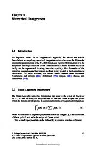
Example 1. The first example is an epidemic model due to Cooke [31]. It describes the fraction of a population that is infected by a virus at time t through the equation dx (t) = bx (t − 7) (1 − x (t)) − cx (t) , dt

t ∈ [0, 70]

(4.2)

Here b and c are positive constants. If b > c, then the solution x (t) = 1 − c/b is an equilibrium point. The equation is integrated for b = 2, c = 1 and initial condition function x (t) = 0.8 for t ∈ [−7, 0].

0.8

0.75

y

0.7

0.65

0.6

0.55

0.5

x(t) = 1−c/b 0.45

0

5

10

15

20

25

30

35

40

45

50

t

Fig. 4.1. Numerical solution for the Example 1 with b = 2, c = 1 obtained by the LL scheme (4.1) with h = 0.01. The straight line represents the equilibrium point x (t) = 1 − c/b.

Figure 4.1 shows the numerical solution converging to the equilibrium point. Figure 4.2 shows the maximum errors of the LL scheme (4.1) in the computation of the solution of the equation (4.2) in (t)h , for h = 0.1, 0.01, 0.001; and the straight line that fit these points in the minimum square sense. The slope of that line is 2, which agrees with the theoretical estimate obtained in the previous section. As ”true” solution was used the trajectory obtained by the LL scheme with h = 0.00001. For a comparison, Figure 4.2 also shows the results obtained by the polynomial LL scheme e , i.e., schemes of the form (2.15) with first and third order interpolating polynomial y with p = 0 and p = 2, respectively. In each case, the slope of their respective lines are 1 and 2, which also agrees with the theoretical estimate. Example 2. The second example is the stiff DDE proposed in [6] to describe the dynamic of an antiviral immune response. The disease dynamic is governed by the

21

LOCAL LINEARIZATION METHOD FOR DDES

−2

−3

log(error)

−4

p=0

−5

−6

p=2 −7

p=1 −8 −3

−2

−1

log(h)

Fig. 4.2. Maximum errors of interpolating polynomial LL schemes produced in the integration of the Example 1 at the points (t)h , with h = 10−1 , 10−2 , 10−3 . The slope of the straight line that fit these points are 1, 2 and 2 for the schemes with interpolating polynomials of grade p = 0, 1, 2, respectively.

system of ten-dimensional DDEs dx1 dt dx2 dt dx3 dt dx4 dt dx5 dt dx6 dt dx7 dt

= a1 x2 + a2 a3 x2 x7 − a4 x1 x10 − a5 x1 − a6 x1 (a7 − x2 − x3 ) = a8 x1 (a7 − x2 − x3 ) − a3 x2 x7 − a9 x2 = a3 x2 x7 + a9 x2 − a10 x3 = a11 a12 x1 − a13 x4 = a14 ((1 − x3 /a7 )a15 x4 (t − τ1 )x5 (t − τ1 ) − x4 x5 ) − a16 x4 x5 x7 + a17 (a18 − x5 ) = a19 ((1 − x3 /a7 )a20 x4 (t − τ2 )x6 (t − τ2 ) − x4 x6 ) − a21 x4 x6 x8 + a22 (a23 − x6 ) = a24 ((1 − x3 /a7 )a25 x4 (t − τ3 )x5 (t − τ3 )x7 (t − τ3 ) − x4 x5 x7 ) − a26 x2 x7

+a27 (a28 − x7 ) dx8 = a29 ((1 − x3 /a7 )a30 x4 (t − τ4 )x6 (t − τ4 )x8 (t − τ4 ) − x4 x6 x8 ) + a31 (a32 − x8 ) dt dx9 = a33 (1 − x3 /a7 )a34 x4 (t − τ5 )x6 (t − τ5 )x8 (t − τ5 ) + a35 (a36 − x9 ) dt dx10 = a37 x9 − a38 x10 x1 − a39 x10 dt with five time delays τ1 = τ2 = 0.6, τ3 = τ4 = 2 and τ5 = 3; and initial conditions

22

J.C. JIMENEZ, L. M. PEDROSO, F. CARBONELL V. HERNANDEZ

x1 (t) = 2.9 × 10−16 , x2 (t) = x3 (t) = x4 (t) = 0, x5 (t) = a18 , x6 (t) = a23 , x7 (t) = a28 , x8 (t) = a32 , x9 (t) = a36 , and x10 (t) = a36 a37 a39 , for all t ∈ [− τ5 , 0]. The parameters ai are given in Table 4.1. Table 4.1 Values of the parameters in the DDE of Example 2 j/a 0 1 2 3 4 5 6 7 8 9

aj − 83 5 6.6 × 1014 3 × 1011 0.4 2.5 × 107 5 × 10−13 2.3 × 109 0.052

a1j 0.15 9.4 × 109 10−15 1.2 2.7 × 1016 2 5.3 × 1027 1 10−18 2.7 × 1016

a2j 2 8 × 1028 1 10−19 5.3 × 1033 16 1.6 × 1014 0.4 10−18 8 × 1032

a3j 16 0.1 10−18 1.7 × 1030 3 0.4 4.3 × 10−22 8.5 × 106 8.6 × 1011 0.043

That equation has been used as a test example to compare the performance of numerical integrators in the case of multidimensional stiff equations with multiple delays. It has been reported in [6] that various of them fail to produce a numerical solution after t = 110 because the appearance of sharp picks in the solution. Figure 4.3 illustrates this problem. In this case, the explicit continouos extension Runge-Kutta (2,3) scheme with step-size h = 0.01 was used.

21

y1 y2 y3

10

0 1021 0 1021 0

124

y4

10

y5

10

0

14

0

276 y6 10

0

y7

1021 0

y8

10280 0

y9

10122 0

y10

10248 0 0

50

100

150

t

Fig. 4.3. Approximate solution of the Example 2 computed by the continuous extention RungeKutta (2,3) scheme with step size h = 0.01.

On the contrary, figure 4.4 shows the numerical solution until t = 150 obtained by the LL scheme (4.1) with the same step-size. Table 4.2 presents the maximum of the relative errors of the LL scheme in (t)h versus h for each variable. As ”true”

23

LOCAL LINEARIZATION METHOD FOR DDES

solution was used the trajectory obtained by the LL scheme with h = 0.00001. The time for computing such solution (until t = 100) was 1.7 longer than the time used by the Runge-Kutta scheme mentioned above. Thus, no small step-size is necessary to integrate that equation with an adequate precision and computational cost, which reveals the potential of the LL method to integrate stiff DDEs.

−11 y1 4x10

0

−13 y2 4x10

y3

0 10−13 0

−16 y4 4x10

y5 y6 y7

0 5x10−17 0 10−17 0 5x10−18 0

y8 4x10−12

0 −15 y9 2x10

0 4x10−8

y

10

0

50

100

150

t

Fig. 4.4. Approximate solution of the Example 2 computed by the LL scheme (4.1) with step size h = 0.01.

Table 4.2 Maximum of the relative errors (%) produced by the LL scheme (4.1) in the integration of the Example 2 on the interval [0, 150] with different step-size h.

h/x 0.1 0.01

1 17.86 0.13

2 0.0377 0.0004

3 0.0478 0.0035

4 0.7256 0.0780

5 0.3140 0.0031

6 0.5269 0.0054

7 1.3753 0.0120

8 0.6410 0.0730

9 0.6258 0.0071

10 1.7621 0.0132

5. Conclusions. Local Linearization approach for the numerical integration of DDEs was introduced and two numerical schemes were considered. The first one, called natural LL scheme, preserves the stability of multidimensional linear DDEs with multiple delays but its computational cost is high in the case that the smallest delay of the DDE be much lower than the final integration time. On the contrary, according to the simulation study carried out, the computational cost of the polynomial LL scheme is comparable with the cost of the conventional explicit integrators but with the advantage of integrating stiff systems. This last result, agrees with similar performance of the LL integrators of other classes of differential equations (ODEs, RDEs and SDEs). The two LL schemes proposed in this paper are explicit and have second order of convergence. Nevertheless, high order schemes of this family can also be derived by just follow the same ideas that have been used to construct high order

24

J.C. JIMENEZ, L. M. PEDROSO, F. CARBONELL V. HERNANDEZ

LL integrators for ODEs and SDEs [15, 16]. 6. Appendix. The following result is a generalization of Theorem 1 in [40]. Lemma 6.1. (Theorem 1 in [11]) Let n, d1 , d2 , ..., dn be positive integers and A a n × n block triangular matrix defined by   A11 A12 ... A1n  0 A22 ... A2n    A = ..  , ..  0 . 0 .  0

0

0

Ann

where (Alj ) are dl × dj matrices, with l, j = 1, ..., n  B11 (t) B12 (t) ...  0 B22 (t) ...  eAt =  ..  0 . 0 0 0 0

. Then for t > 0  B1n (t) B2n (t)   ..  , .  Bnn (t)

with Bll (t) = eAll t , l = 1, ..., n Zt Blj (t) = M(l,j) (t, s1 )ds1 , l = 1, ..., n − 1, j = l + 1 0

Zt M(l,j) (t, s1 )ds1

Blj (t) = 0

+

t s1 j−l−1 X Z Z k=1 0

0

Zsk ...

X

M(l,i1 ,...,ik ,j) (t, s1 , ..., sk+1 )dsk+1 ...ds1 ,

0 l