Aug 27, 2007 - Vishal Sood1, 2 and Peter Grassberger1, 2. 1Complexity Science ..... 06625 (2006). [10] R. Lyons, R. Pemantle, and Y. Peres, Probab. Theory.
Localization Transition of Biased Random Walks on Random Networks Vishal Sood1, 2 and Peter Grassberger1, 2
arXiv:cond-mat/0703233v3 [cond-mat.stat-mech] 27 Aug 2007
2
1 Complexity Science Group, University of Calgary, Calgary, Canada Institute for Biocomplexity and Informatics, University of Calgary, Calgary, Canada (Dated: February 6, 2008)
We study random walks on large random graphs that are biased towards a randomly chosen but fixed target node. We show that a critical bias strength bc exists such that most walks find the target within a finite time when b > bc . For b < bc , a finite fraction of walks drifts off to infinity before hitting the target. The phase transition at b = bc is a critical point in the sense that quantities like the return probability P (t) show power laws, but finite size behavior is complex and does not obey the usual finite size scaling ansatz. By extending rigorous results for biased walks on Galton-Watson trees, we give the exact analytical value for bc and verify it by large scale simulations. PACS numbers: 02.70.Uu, 05.10.Ln, 87.10.+e, 89.75.Fb, 89.75.Hc
Random walks are a fascinating subject, both for their intrinsic mathematical beauty and for their wide range of applications [1]. One of the most celebrated results is that unbiased random walks on regular lattices are recurrent for dimension d ≤ 2, while they are transient for d > 2 [2]. This means that a walk starting at a node x certainly returns to x when d ≤ 2, but has a finite chance to escape to infinity when d > 2. Here we study an analogous problem for walks on random graphs which lack small loops in the limit of infinite graph size. Examples of such graphs include the Erd¨ osRenyi (ER) random graphs, as well as random graphs with any fixed degree sequence, provided that the variance of the degree distribution is finite. We call the latter Molloy-Reed (MR) graphs [3]. An ER graph with N nodes is constructed by introducing a link between each pair of nodes with probability p. It is in many ways similar to an infinite dimensional lattice. In particular, its diameter l increases only logarithmically with the number of nodes, while N ∼ ld on a d-dimensional lattice. Thus one should expect unbiased random walks on an ER graph to be transient. Although less is known rigorously about MR graphs, we expect the same to be true for them. In order to arrive at a non-trivial problem, we thus consider walks biased towards a randomly chosen but fixed “target” node. We show that there is a phase transition from recurrence (or localization) to delocalization at a critical bias strength. Notice that this is unrelated to similar phase transitions observed e.g. in [4], where the bias is not towards but away from the target. This seemingly abstract mathematical problem has a number of practical applications. Consider, e.g., routing a message from node A to node B on the internet. Each node i maintains a routing table which indicates for each target node the optimal first step, parting from i. Using her routing table, A sends the message to her optimal neighbor i1 . From there it is sent, using the routing table at i1 , to i2 , etc., until in = B is reached. If all routing tables are correct and up-to-date, the message reaches its destination along the optimal path (i.e., the path between A and B with the shortest length). However, some routing tables may be faulty, either because
they contain mistakes or have become obsolete due to changes in the internet topology. If the fraction of such nodes is below a certain threshold, the effect is small and routing is still efficient: the average time to go from A to B scales linearly with the distance. But when the fraction exceeds a critical value, the message might take a very long and convoluted path through a finite fraction of the entire network, before reaching its destination. There are of course many details in which routing on the real internet differs from the simpler problem of biased random walks on random graphs [5]. For instance, the degree distribution of the internet is approximately scale-free with a divergent second moment [6]; stray messages on the internet are killed after some time; and the bias is implemented differently and is quenched (the same routing tables are used at successive time steps). Despite these technical details, the two problems are basically the same. For a related discussion of communication based on noisy routing, see [7]. Another application is to quantum mechanics. A random walker on a graph corresponds quantum mechanically to a particle with hopping dynamics. The recurrence problem for an unbiased walk corresponds then to the question whether such a particle, subjected to an attractive δ-potential concentrated on a single node, forms a bound state. Localization of biased random walks corresponds to the existence of bound states for potentials which increase linearly with distance from the target node. Delocalization would imply the paradoxical situation that no bound state exists, although the potential increases forever as one goes further away from the target node. Instead, a particle released near the bottom of the potential continues to climb up the potential forever, because there are always more paths leading uphill than leading back to the bottom. Technically, we define our walks as follows. Consider a finite but large undirected random graph G with N nodes and with degrees chosen from a distribution PG (k). We assume that PG (k) is such that G is sparse and has a giant connected component (GC). We define the distance between any two nodes as the number of links in the shortest path connecting them. We randomly choose a
2 node A on G and label all other nodes according to their distance from A. Consider node i at distance di from A, which has ki− , ki0 and ki+ neighbors at distances di + 1, di − 1, and di from A, respectively. The random walk steps from i with probabilities p− i =
b , Ni
p0i =
1 , Ni
p+ i =
b−1 . Ni
(1)
to a node closer to, at the same distance as or further away from A, respectively. Finally, normalization requires Ni = bki− + ki0 + b−1 ki+ . Similar walks on regular lattices have been studied repeatedly, see e.g. [8]. More importantly, Eq. (1) is a generalization of the bias used in the ‘λ-biased random walks’ studied on Galton-Watson (GW) trees [9, 10, 11]. Starting at the root, each node on the tree has a number of daughter nodes chosen from a prescribed distribution. The root is chosen as the target A of the random walk. On a tree, every node i 6= A has only one neighbor closer to the target, ki− = 1, and no neighbors at the same distance, ki0 = 0. The probabilities of the next step are + chosen such that [9, 10] p− to i /pi = λ. This corresponds √ Eq. (1), restricted to tree-like graphs, with b = λ. The typical length of a loop in an undirected graph G with finite mean degree and finite degree variance is of order ln N [12, 13]. If only local properties are of interest, the graph can, as N → ∞, be effectively replaced by a GW tree. However, a subtlety should not be overlooked: to obtain a rooted tree T from a loopless undirected graph G, we have to choose randomly a node A as the root of the tree, and draw an arrow on each link pointing away from A. A node with degree k on G has in-degree 1 and out-degree k − 1 on the effective tree. The out-degree distribution on the tree can be related to the degree distribution PG (k) of the graph [3], PTout (k + ) =
k PG (k), hki
(2)
with k = k + + 1. The prefactor k/hki on the right hand side takes into account the fact that each of the k links attached to the node can play, with the same probability, the role of the incoming link on the tree. A GW tree will grow to infinity only if its average out-degree is larger than 1 [14]. This implies that the underlying random graph is connected when [3, 15] µ = hk + iGW = hk(k − 1)iG /hkiG > 1,
(3)
which we assume to be satisfied. Further for the graph to be sparse and lack small loops we assume that µ ≪ N . If there is a critical bias λc for walks on a GW tree so that walks are localized near the root for λ > λc and delocalized for λ < λc , then an analogous critical bias √ bc ≤ λc must also exist for graphs. The reason is simply that only local properties are relevant when the walks are localized [18]. Hence localization on a GW tree implies localization on the corresponding graph. Conversely, as-
√ sume that bc were strictly smaller than λc . Then walks on the GW tree with b2c < λ < λc would also be localized, contradicting the starting assumption √ that the critical point is at λc . Thus we must have bc = λc . Indeed, it is known that the λ–biased random walk on a GW tree has a localization transition at λc = µ, such that the walk is recurrent for λ > λc and transient for λ < λc [11]. For λ = λc the authors of [9] prove a central limit theorem which states that the walk behaves, as far as the distance from the root is concerned, like unbiased 1-d Brownian motion. In the following we will summarize the arguments leading to those conclusions and indicate modifications required to apply to ER and MR graphs. For a walker at a node i that is different from the root A, we define pE i to be the probability that it escapes to infinity before it hits the root. We denote by P(i) the set of parents of i, i.e. the neighbors that are closer to A than i. Similarly, S(i) is the set of siblings of i (i.e. dj = di for all j ∈ S(i)), and C(i) denotes its children. Finally, we define pE A = 0. Then we have, for any i 6= A, X X X 1 1 . (4) b pE pE pE pE i = j + j + j Ni b j∈S(i)
j∈P(i)
j∈C(i)
Using Ni defined after Eq. (1) we can rearrange this to X
j∈P(i)
E (pE i − pj ) =
1 X E 1 X E E (pj − pE (p − p ) + i ). j i b2 b j∈S(i)
j∈C(i)
(5) A sum over all i with fixed di = d, cancels all the contributions of the siblings. Defining X E (pE (6) Xd = i − pj ) , i: di =d j∈P(i)
we get the recursion Xd =
1 Xd+1 . b2
(7)
which can be iterated to give the average escape probability from all children of the root pE ≡
1 1 X E pi = Xd+1 . kA kA b2d
(8)
i∈C(A)
For trees this simplifies because each node (except for the root) has only one parent, and the number of terms on the r.h.s. increases in average as µd for large d. Since each term is bounded, the total sum increases at most as (µ/b2 )d . Thus pE = 0 for b2 > µ, showing that the walk √ is recurrent. The proof that bc is not only ≤ µ, but √ (9) bc = µ , is found in [11]. Basically, one replaces in Eq. (8) the number of terms by its expected value and the difference
3 E pE i − pj by its average hpid+1 − hpid , to obtain
35
hpid = α − β
�
� 2 d
b µ
(11) 2
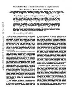
with α and β being constants. For b > µ, the only consistent values are α = β = 0. For b2 < µ one has a non-zero solution, indicating pE > 0. For general finite MR graphs the number of nodes at distance d from the root increases slower than µd , due to √ the existence of loops. In this case bc ≤ µ holds a for√ tiori, but the rigorous proof that also bc ≥ µ becomes d more difficult. The corrections to µ are small for small d (there are few small loops), and we can expect that the effect of loops on bc can be neglected in the limit N → ∞. But loops should effect the finite size scaling behavior. To verify the existence of a localization transition on large ER graphs, check Eq. (9), and study finite size effects, we perform large scale numerical simulations. We first generate large ER graphs (with up to 2×10⁸ nodes), for several nominal values of hki. These are chosen such that the GC contains more than 90% of all nodes. Pruning all nodes and links not connected to the GC gives the final graph size N . This procedure increases hki slightly and makes the degree distribution slightly nonPoissonian, so that µ no longer coincides with the naive theoretical estimate µ = hki for ER graphs. Instead, it is estimated from the exact definition Eq. (3). After extracting the GC, we choose randomly one of its nodes as the target A and compute every other node’s distance from A. Then we start M walks at A and follow them until they return to A. This is repeated M ′ times by taking new target nodes, and finally the whole procedure is repeated for M ′′ different graphs. The first observable to be discussed is the average return time. For b = 1, i.e. for unbiased random walks, the average return time hti on a finite graph with N nodes is ∝ N [12], We expect the same to hold for all 1 ≤ b < bc . For the critical bias b = bc , since the distance of the biased walk from the root behaves as a 1-d Brownian motion, the return time should grow as logN which is the diameter of the graph. In contrast, limN →∞ hti < ∞ in the localized regime b > bc . In Fig. 1 we show hti versus N for various biases on a linear-log scale. The nominal number L/N of links per node in constructing the ER graphs was 7/3, which would give µ = 14/3 = 4.6667. For the GC, we found numerically µ = 4.6673. The critical bias should be bc = 2.1604, which certainly agrees with with Fig. 1. More significant is the distribution of return times. In the inset of Fig. 2 we plot (not normalized) histograms of return times P (t) against t for walks with various values of b, on the GC of an ER graph with N = 2 × 10⁸ and
b = 2.00 b = 2.10 b = 2.15 b = 2.20 b = 2.30
30 25
bcrit = 2.16
20 15 10 5 101
102
103
104
105
106
107
108
N
FIG. 1: (color online) Average return times against the system size N for different values of the bias b, on ER graphs with hki = 14/3.
10
9
8 x 10
6 x 10
8
P(t)
which has the solution
average return times
(10)
P(t) [not normalized]
b2
(hpid+1 − hpid )
8
10
7
10
5
10
3
even t odd t
10 10
10
2
10
3
b = 1.65
3/2
� µ �d
t
pE ∼
4 x 10
8
3 x 10
8
b = 1.93 10
100 return time t
1000
FIG. 2: (color online) Histograms of return times for walks on ER graphs with N = 2 × 10⁸ and L/N = 1.5. Shown is t3/2 P (t) where P (t) is the return probability. The inset is the plot of P (t). The critical curve (third curve from above) is the one which is flattest at t ≈ 100. Each curve corresponds to a fixed bias b, with steps of 0.04. The upper (red) curves correspond to even t, the lower (blue) ones to odd t.
L/N = 1.5. For this graph bc = 1.73542. The most striking observation is a very large even/odd effect for small t: Compared to the values for even t, P (t) is nearly zero for odd t, an immediate consequence of the suppression of small loops. On a loopless tree, return times are always even. Conversely, we can assume that loops are negligible for even times for which P (t ± 1) ≪ P (t). In this regime we should thus expect that the result for GW trees applies, i.e. P (t) ∼ t−3/2 at the critical bias. This prediction (which is the same as for unbiased 1-d random walks [9]) is in complete agreement with our data, as seen from Fig. 2. Fig. 2 also indicates the complicated finite-size behavior. P (t) is not convex at the critical
4 2.0 1.8 1.6 1.4
ρ(d)
1.2 1.0 .9 .8 b = 1.69 b = 1.71 b = 1.73 b = 1.75 b = 1.77
.7 .6 .5 2
4
6
8
10 d
12
14
16
18
20
FIG. 3: (color online) Density of walkers against distance from the target, for five values of b close to criticality.
point, and the usual finite size scaling ansatz (power law times homogeneous function) does not hold. Finally, if critical walks resemble unbiased 1-d Brownian motion, with reflecting boundaries at d = 0 and at d ≈ ln N [9], then the density ρ(d) of walkers per launch, integrated over all times, should be constant at b = bc . Fig. 3 shows that ρ(d) is indeed flat, to very high accuracy, for b = 1.732 ± 0.002. This agrees with the exact bc within two standard deviations, and gives the most precise numerical verification of the theoretical prediction. We have shown that walks on a random graph biased towards a given node show a localization/delocalization transition, corresponding to a transition from recurrent to transient behavior. If routing is noisy but the noise level is below a critical threshold, the walks are able to reach their destination in a finite amount of time. This resilience of the walks can be taken into account while designing routing strategies for the internet or
[1] B. D. Hughes, Random walks and random environments, Vol. 1 (Oxford University Press, New York., 1995), 1st ed. [2] G. Polya, Mathematische Annalen 84, 149 (1921). [3] M. Molloy and B. Reed, Random Struct. Algor. 6, 161 (1995). [4] D. Dhar, J. Phys. A: Math. Gen. 17, L257 (1984). [5] W. Willinger, R. Govindan, S. Jamin, V. Paxson, and S. Shenker, PNAS 99, 2573 (2002). [6] A.-L. Barabasi and R. Albert, Science 286, 509 (1999). [7] M. Rosvall and K. Sneppen, Europhys. Lett. 74, 1109 (2006). [8] V. Mehra and P. Grassberger, Physica D 168, 244 (2002). [9] Y. Peres and O. Zeitouni, e-print arXiv:math.PR/0606625 (2006). [10] R. Lyons, R. Pemantle, and Y. Peres, Probab. Theory
other traffic problems with noisy dynamics. The localization/transition should also be related to a curious effect in quantum mechanics on random graphs with linearly rising potentials, where we expect a paradoxical “unbinding” transition when the potential becomes too shallow. Our numerical studies have only included ER graphs, mainly because these can be easily generated even with very large sizes. However, we expect the existence of a delocalization transition to be robust and to hold for any degree distribution with a finite second moment. For scale free graphs, P (k) ∼ 1/k γ with γ ≤ 3, the second moment diverges with N , leading formally to bc = ∞. For scale free graphs, the number of nodes within distance d from the target does not grow exponentially, ∼ µd as assumed in Eq. (10). It rather grows superexponentially as exp(exp(d)) [16, 17]. To compensate this, the critical bias has to be distance-dependent, growing also super-exponentially with d. Alternatively, if we describe the finite-size behavior by an N -dependent but d-independent effective critical bias bc (N ), then this has to grow as a power of N . Finally, we should point out that our theoretical prediction for bc holds only for a very particular type of bias, given by Eq. (1). For other biases we expect the transition to show the same scaling laws (as long as the bias strength is independent of d), although we can no longer predict the exact location of the phase transition. The same is true for graphs with many small loops, including those often observed in real world networks. If the bias strength increases (decreases) with d beyond limit, then one has always (de)-localisation for graphs with a finite second-moment of the degree distribution and with exponential growth of the number of neighbors with distance. We want to thank Maya Paczuski for numerous discussions and for careful reading of the manuscript. VS would like to thank Orion Penner for checking the calculations. PG thanks iCore for financial support.
Relat. Fields 106, 249 (1996). [11] R. Lyons, Ann. Probab. 18, 931 (1990). [12] B. Bollob´ as, Modern Graph Theory, Graduate Texts in Mathematics (Springer-Verlag, Berlin, 1998). [13] S. Janson, T. Luczak, and A. Ruci´ nski, Random Graphs (John Wiley & Sons, Inc., New York, 2000). [14] S. Athreya, Branching Processes (Birkhausser, 1960). [15] R. Cohen, K. Erez, D. ben Avraham, and S. Havlin, Phys. Rev. Lett. 85, 4626 (2000). [16] F. Chung and L. Lu, PNAS 99, 15879 (2002). [17] R. Cohen, and S. Havlin, Phys. Rev. Lett. 90, 058701 (2003). [18] Notice that this argument is not strictly correct, since it neglects the exponentially small probability for delocalized walks even when λ > λc .