were confirmed by experimental observations of lock-exchange flows in a tube of .... be a driving force throughout the entire stratified-flow region. This situation ...
c 2007 Cambridge University Press J. Fluid Mech. (2007), vol. 577, pp. 53–77. � doi:10.1017/S002211200600437X Printed in the United Kingdom
53
Lock-exchange flows in sloping channels V. K. B I R M A N1 , B. A. B A T T A N D I E R1,2 , E. M E I B U R G†1 A N D P. F. L I N D E N3 1
Department of Mechanical Engineering, University of California, Santa Barbara, CA 93106, USA 2 Ecole Polytechnique, 91128 Palaiseau Cedex, France 3 Department of Mechanical and Aerospace Engineering, University of California, San Diego, CA 92093, USA
(Received 10 March 2006 and in revised form 17 October 2006)
Two-dimensional variable-density Navier–Stokes simulations have been conducted in order to investigate the effects of a slope on the classical lock-exchange flow. Simulations of full lock releases show that the flow goes through an initial quasisteady phase that is characterized by a constant front velocity. This quasi-steady front velocity has a maximum for slope angles around 40◦ , and it persists up to a dimensionless time of the order of 10. The flow subsequently undergoes a transition to a second phase with a larger, unsteady, front velocity. These computational findings were confirmed by experimental observations of lock-exchange flows in a tube of circular cross-section. The reason for the observed transition from a quasi-steady front velocity to a larger, unsteady, value is found in the continuous acceleration of the stratified fluid layers connecting the two fronts by the streamwise component of the gravity vector. This acceleration leads to a situation where the fluid layers behind the current front move faster than the front itself. Initially the resulting addition of fluid to the current front from behind affects only the size of the front, while its velocity remains unchanged. Eventually, the current front is unable to absorb more fluid from behind and its velocity has to increase, thereby triggering the transition to the second, unsteady, phase. The transition time is determined as a function of the slope and the density ratio of the two fluids. For increasing density contrast, the transition is seen to occur earlier for the denser current. Conceptually simple models based on the analysis by Thorpe (1968) are compared with simulation results for the flow in the region connecting the fronts. For the early stages of the flow a two-layer stratification model is found to be appropriate, while the later stages require a three-layer stratification model, owing to the intense mixing in the central part of the channel cross-section. These models are employed to estimate the time after which the accelerating stratified fluid layers will affect the velocities of the current fronts. They provide upper and lower estimates for the transition time which are in good agreement with the simulation results.
1. Introduction Gravity currents, sometimes also called density or buoyancy currents, form as a result of predominantly horizontal density gradients in fluids. They play a central role in a variety of geophysical situations and industrial applications, as described in † Author to whom correspondence should be addressed.
54
V. K. Birman, B. A. Battandier, E. Meiburg and P. F. Linden
the comprehensive introduction to this topic by Simpson (1997). The lock-exchange set-up has long served as a paradigm configuration for studying the spatio-temporal evolution of gravity currents. Among the first authors to address this geometry, Huppert & Simpson (1980) demonstrated the existence of three distinct phases in lock-exchange flows over horizontal surfaces; see also the related experimental investigations of Britter & Simpson (1978) and Simpson & Britter (1979). The initial phase is characterized by a gravity current propagating with a constant front velocity. Once the disturbance generated by the endwall overtakes the front, the slumping phase gives way to a self-similar inertial phase during which the front slows down (Rottman & Simpson 1983). Eventually a phase is reached in which the buoyancy forces are balanced by viscous forces. For full-depth lock releases the initial constant-front velocity is generally well captured by the classical energy-conserving theory of Benjamin (1968). For a critical discussion of Benjamin’s analysis, along with an alternative theory, the reader is referred to the recent work of Shin, Dalziel & Linden (2004). A central question of the present study is how the above well-established succession of distinctly different phases is modified by the presence of a sloping bottom. This initial series of lock-exchange investigations was subsequently extended in several different directions. Hallworth et al. (1993) developed a new pH-based method to study entrainment in turbidity currents. They showed by dimensional analysis that the entrainment of ambient fluid in gravity currents depends only on the initial lock volume and the distance from the release location. The work was extended further to two-dimensional and axisymmetric turbulent gravity currents in Hallworth et al. (1996). Hacker, Linden & Dalziel (1995) studied the effect of the lock’s aspect ratio on the entrainment rate for gravity currents on a horizontal surface. They also discussed the development of different internal structures due to differences in the entrainment rate. The direct numerical simulations of H¨artel, Meiburg & Necker (2000) and Cantero et al. (2006) provide highly resolved information on mixing and dissipation. The lock-exchange experiments Gr¨ obelbauer, Fanneløp & Britter (1993) focus on non-Boussinesq effects, as do the more recent theoretical (Lowe, Rottman & Linden 2005) and numerical (Birman, Martin & Meiburg 2005; Etienne, Hopfinger & Saramito 2005) modelling efforts. In these studies, strong density differences are seen to result in distinctly different front heights, propagation velocities and overall dynamics for the light and the heavy fronts. When the driving force is provided by particle loading rather than compositional variations, a host of new phenomena arise, as discussed in the investigations by Bonnecaze, Huppert & Lister (1993), Bonnecaze & Lister (1999) and Necker et al. (2002, 2005). Such particle-driven flows frequently occur over sloping bottoms, e.g. in the form of powder snow or pyroclastic avalanches or as sediment-driven turbidity currents that propagate from the continental shelf down the continental slope to the deep ocean. These examples differ from lock-exchange situations in that they are not confined by side or top walls, so that the flow domain is essentially infinite. The propagation of a given volume of heavy fluid down a slope should thus proceed in a self-similar fashion, a fact that was confirmed by the investigation of Beghin, Hopfinger & Britter (1981). By coupling scaling laws for the balance of inertial and buoyancy forces with mass-conservation arguments that include the effects of entrainment, these authors were able to derive a closed-form similarity solution. The theory predicts the velocity of the centre of mass to increase initially and to decrease during the later stages of the flow. The theoretical solutions for both these phases are in good agreement with corresponding experimental observations. This problem has been revisited recently by Maxworthy & Nokes (2006), who found that for larger
Lock-exchange flows in sloping channels
55
buoyancy releases the dynamics become more complicated, owing to the interaction of the current front with the trailing sections of the fluid. These authors employed dimensional analysis in order to arrive at a more refined description of the flow. Webber, Jones & Martin (1993) and Tickle (1996) presented similarity solutions to the shallow-water equations and proposed wedge models for three-dimensional gravitycurrent releases on slopes. Ross, Linden & Dalziel (2002) performed corresponding experiments and extended the wedge models to include the effects of entrainment. Some applications of gravity currents down inclined slopes are appropriately described by the lock-exchange geometry, such as the propagation of accidentally released methane in a mine, the ventilation of vehicular tunnels and the spreading of hot products resulting from a tunnel fire. Earlier investigations of gravity currents in sloping channels include that by Ellison & Turner (1959), who measured the entrainment as a function of the Richardson number. Britter & Linden (1980) focused on the head of a gravity current in an inclined deep channel. Importantly, they investigated the situation produced by a continuous supply of dense fluid, which is different in some aspects from the full-depth finite-release lock-exchange flow studied here. Britter & Linden (1980) reported that the current front propagates at an approximately constant velocity for all but very small angles. The authors furthermore noted that the head size increases not only by entrainment from the ambient but also as a result of flow into the head from the trailing portions of the current. In lock-exchange flows, a region of stably stratified shear flow forms throughout the central section of the channel, where the lighter fluid is situated above the heavier. In a horizontal channel, this flow is driven by ‘end effects’ only, i.e. by the conditions outside the central section. For a sloping bottom, however, gravity continues to be a driving force throughout the entire stratified-flow region. This situation was investigated by Thorpe (1968, 1971), although in his experiments it was approached from a set of initial conditions that, in some sense, were diametrically opposed to the lock-exchange configuration. The initial set-up in Thorpe (1968) consisted of a horizontal channel with closed ends containing a stably stratified fluid at rest. After the channel was tilted, a continuously accelerated stratified shear flow evolved in the central section of the channel that persisted until it was modified by surges propagating from the endwalls. The author presented a unidirectional flow model for the stratified shear flow which was in good agreement with the experimental observations until the onset of a shear-driven Kelvin–Helmholtz instability, which was further studied theoretically in Thorpe (1971). Parts of the flow model developed by Thorpe (1968) will be employed in the present investigation. The paper is structured as follows. Section 2 describes the physical problem and the set-up for the simulations, along with the governing equations and the boundary and initial conditions. The computational approach is briefly outlined in § 3. Section 4 presents the simulation results. Both the height and velocity of the front will be analysed, along with the ensuing mixing, as functions of the slope angle and the density ratio. Experimental data for the front velocity will be presented in § 5. The simple model of Thorpe will be adapted, in § 6, to explain certain aspects of the simulation results. A brief summary section concludes the paper. 2. Problem formulation The investigation focuses on a rectangular channel of height H and length L (figure 1) which is filled with two miscible fluids that are initially separated by a membrane located at a distance L1 from the left-hand wall. The x-axis is parallel to
56
V. K. Birman, B. A. Battandier, E. Meiburg and P. F. Linden
z ρ1
H
g
ρ2
x L1
L = L1 + L2
L2 θ
Figure 1. The lock-exchange configuration in a sloping channel. A membrane initially divides the rectangular container of length L and height H into two compartments of length L1 and L2 = L − L1 . The left-hand chamber is filled with fluid of density ρ1 , while the right-hand chamber contains fluid of density ρ2 . The container is tilted at an angle θ with respect to the horizontal. Upon removal of the membrane, a dense front moves rightwards along the lower boundary, while a light front propagates leftwards along the upper boundary.
the sloping bottom, while the left- and right-hand endwalls point in the z-direction. The fluid in the left-hand compartment has density ρ1 , and the right-hand reservoir holds a fluid of density ρ2 < ρ1 . This initial configuration causes a discontinuity of the hydrostatic pressure across the membrane, which sets up a flow predominantly in the x-direction once the membrane is removed. The denser fluid moves rightwards along the bottom of the channel, while the lighter fluid moves leftwards along its top. For the analysis of the resulting flow, we employ the incompressible variabledensity Navier–Stokes equations without invoking the Boussinesq approximation; see Birman, Martin & Meiburg (2005). The buoyancy velocity � ρ1 − ρ2 (2.1) ub = g � H with g � = g ρ1 is taken as the characteristic velocity and H as the representative length √ scale; the larger density ρ1 serves as the characteristic density. Alternatively, ub = g � H /cos θ can be employed as the characteristic velocity; see S´eon, Hulin & Salin (2005). This scaling can be useful for capturing the effects of relatively small angles when the current travels faster. However, it results in unreasonably large characteristic velocities for larger values of θ and in ub → ∞ for θ → 90◦ . Since the present investigation will not be limited to small angles, we employ the characteristic velocity ρ1 , which does not depend on the angle. In dimensionless form the governing equations thus read 1 Dρ + ∇ · u = 0, ρ Dt Du 1 1 ρ = ρeg − ∇p + ∇ · (2ρ S), Dt 1−γ Re 1 2 Dρ = ∇ ρ. Dt Pe
(2.2) (2.3) (2.4)
Lock-exchange flows in sloping channels
57
Here D/Dt denotes the material derivative of a quantity, u = (u, w)T indicates the velocity vector and p the pressure; eg = (sin θ, −cos θ) represents the unit vector pointing in the direction of gravity, γ = ρ2 /ρ1 is the density ratio, S denotes the rate-of-strain tensor and θ is the angle of inclination of the channel bottom with respect to the horizontal direction; see figure 1. It is instructive to conduct an order-of-magnitude analysis of the terms in the continuity equation (2.2); see also the discussion in Joseph & Renardy (1992). Equation (2.4) suggests that, in dimensional quantities, ∂ 2ρ ρ Dρ ∼ κ 2 ∼ κ 2, (2.5) Dt ∂x δ where δ is the thickness of the layer over which the density varies. This thickness is determined by the balance of strain and diffusion: ρ
∂ 2ρ ∂u ∼ κ 2. ∂x ∂x
With ∂u/∂x ∼ ub /H , this yields
(2.6)
�
κH . (2.7) ub Hence, in the continuity equation (2.2), (1/ρ)Dρ/Dt is formally of the same order as ∂u/∂x. However, the term (1/ρ)Dρ/Dt is confined to the thin concentration boundary layers, of thickness δ; it approaches zero everywhere else. Furthermore, since ∂ 2 ρ/∂x 2 changes sign across the concentration layer, it involves a positive and a negative contribution within the layer. For thin-concentration boundary layers, these contributions cancel each other approximately, resulting in an even smaller far-field effect. Since δ scales as δ (2.8) ∼ Pe−1/2 , H the region over which the term (1/ρ)Dρ/Dt is non-zero decreases as Pe increases. Clearly, in the limit Pe → ∞, i.e. in the absence of diffusion, the substantial derivative vanishes everywhere. The above argument shows that for high-Pe flows, everywhere outside-narrow the concentration boundary layers, the velocity-derivative terms balance each other in the continuity equation while the material-derivative term enters into this balance only within the concentration boundary layers. Hence, omitting the material-derivative term in the continuity equation is justified for high-Pe flows, on which our current interest focuses. Consequently, we employ the simplified set of dimensionless equations δ∼
∇ · u = 0, (2.9) 1 1 Du = ρeg − ∇p + ∇ · (2ρ S), (2.10) ρ Dt 1−γ Re Dρ 1 2 (2.11) = ∇ ρ. Dt Pe In further support of this approach, we note that in all our simulations the initial mass of the denser fluid was conserved to within one half of one per cent, even over long times. Finally, earlier simulations based on the same formulation (Birman et al. 2005) and corresponding experimental data showed excellent agreement. The fluids are assumed to have identical kinematic viscosities ν. Besides γ , the Reynolds number Re and the P´eclet number Pe appear in the above equations; they
58
V. K. Birman, B. A. Battandier, E. Meiburg and P. F. Linden
are defined as ub H ub H , Pe = , (2.12) ν κ where κ represents the constant diffusion coefficient of the two fluids. They are related by the Schmidt number ν (2.13) Sc = , κ which represents the ratio of kinematic viscosity and molecular diffusivity. Test calculations showed the effect of variations in Sc to be very small, so that we took Sc = 1 for all cases; see also Necker et al. (2005). A detailed discussion of the above governing equations is given in Birman et al. (2005) and will not be repeated here. For the purpose of performing two-dimensional numerical simulations, we recast the above equations (2.9) and (2.10) into the streamfunction–vorticity (ψ, ω) formulation. With ∂w ∂u − , (2.14) ω= ∂x ∂z ∂ψ , (2.15) u= ∂z ∂ψ , (2.16) w=− ∂x we obtain Re =
∇2 ψ = −ω, 1 2 ρz ρz Du ρx Dw Dω ρx = ∇ ω− cos θ − sin θ + − Dt Re (1 − γ )ρ (1 − γ )ρ ρ Dt ρ Dt 1 {2ρx ∇2 w − 2ρz ∇2 u + 4ρxz wz + (uz + wx )(ρxx − ρzz )}. + ρRe
(2.17)
(2.18)
We have ψ = 0 along all boundaries. We will investigate both slip and no-slip boundary conditions along all walls, resulting in corresponding boundary conditions for the vorticity field. The normal derivative of the concentration vanishes along all walls, thus enforcing zero diffusive mass flux. 3. Computational approach The simulations employ equidistant grids in a rectangular computational domain. A Fourier spectral approach is used for the streamfunction and vorticity variables in the streamwise x-direction: � ψˆ l (z, t) sin(lαx), (3.1) ψ(x, z, t) = l
ω(x, z, t) =
�
ωˆ l (z, t) sin(lαx),
(3.2)
l
where 2π N1 , α= . (3.3) 2 L Here N1 denotes the number of grid points in the x-direction. The z-derivatives are approximated by compact finite differences; see Lele (1992). As in the Boussinesq |l|
500, our simulations show t ∗ to be nearly independent of Re. However, for Re = 200 no transition is observed in a simulation that was carried on until t = 22. Evidently at this low value of Re viscous forces are sufficiently strong to suppress the increase in the front velocity.
64
V. K. Birman, B. A. Battandier, E. Meiburg and P. F. Linden Simulations Scaling Two-layer model Three-layer model
60 50 40 t*
30 20 10
0
10
20
30
40
50
60
70
θ
Figure 6. The transition time t ∗ at which the front velocity increases from its quasi-steady state to a higher, unsteady, value, as a function of the slope angle for Boussinesq flows with γ = 0.998 and Re = 4000. For comparison, the scaling law (4.1) with a suitable proportionality factor is shown. The dashed line gives the upper estimate obtained from the three-layer model discussed later in the text, while the dotted line provides the lower limit obtained from the two-layer model. The upper limit is more accurate for larger angles, while the lower limit is more accurate at smaller angles.
1.2 1.0 0.8 uq
0.6 0.4 Light front Dense front
0.2
0
0.1
0.2
0.3
0.4
0.5 γ
0.6
0.7
0.8
0.9
1.0
Figure 7. The quasi-steady dimensionless front velocities of the dense and light fronts, respectively, as functions of the density ratio γ for a slope of 30◦ . Similarly to the horizontal case (Birman et al. 2005), the velocity of the dense front (triangles) grows as the density contrast increases while the velocity of the light front (circles) does not depend on γ .
4.3. Influence of the density ratio Both Lowe, Rottman & Linden (2005) and Birman et al. (2005) found that the dimensionless speed of the dense front increases with the density contrast, while the dimensionless speed of the light front remains essentially unchanged; see also the earlier investigations by Keller & Chyou (1991) and Gr¨ obelbauer et al. (1993). The quasi-steady front velocities for non-Boussinesq flows in sloping channels show a similar trend; see figure 7. The qualitative nature of this observation is identical for all angles, although only the representative case of θ = 30◦ is shown here. Lowe et al.
65
Lock-exchange flows in sloping channels 1.8 Light front Dense front
1.6 1.4 1.2 Uf
1.0 0.8 0.6 0.4 0.2 0
3
6
9
12
15
t
Figure 8. Front velocities vs. time for γ = 0.4, θ = 40◦ and Re = 4000. Solid line, dense front; dashed line, light front. The transition occurs earlier, and is more pronounced, for the dense front. 16
30° dense front 30° light front 40° dense front 40° light front 50° dense front 50° light front
14
12 t* 10
8
6 0.3
0.4
0.5
0.6
γ
0.7
0.8
0.9
1.0
Figure 9. Transition times for dense (dashed lines) and light (solid lines) fronts at angles θ = 30◦ (squares), 40◦ (triangles) and 50◦ (circles), as functions of the density ratio. For all density ratios and angles, the transition occurs earlier for the dense front.
(2005) and Birman et al. (2005) furthermore observed that the height of the light front remains unchanged, while that of the dense front decreases with increasing density contrast. Here we find that these observations remain valid for flows on slopes. Figure 8 shows the front velocity for a non-Boussinesq flow with γ = 0.4 on a slope θ = 40◦ . We observe that the transition from the quasi-steady velocity to a higher, unsteady, velocity is quite pronounced for the heavy front, whereas for the light front the increase is hardly noticeable and occurs at a later time. Results from corresponding simulations for a variety of density ratios are summarized in figure 9, which depicts the transition time t ∗ as function of the density ratio for both fronts. 4.4. Mixing Figure 2 demonstrated a profound influence of the slope angle on the vortical structures along the interface. In particular, large-scale interfacial turnover events
66
V. K. Birman, B. A. Battandier, E. Meiburg and P. F. Linden 0.50 0.25 z 0 –0.25 –0.50
(a) 0
4
8
12
16
20
24
16
20
24
28
x 0.50 0.25 z 0 –0.25 –0.50
(b) 0
4
8
12
28
x
Figure 10. The mixing behaviour of the flows shown in figure 2: the mixed regions (shown in black), as defined by (4.4) at time t = 9, for (a) the horizontal and (b) the θ = 30◦ configurations. The mixed region is observed to grow much more rapidly for the sloping lock-exchange flow. 18 10° no-slip 20° no-slip 30° no-slip 40° no-slip 10° slip 20° slip 30° slip 40° slip
15 12 A 9 6 3 0
5
10
15
20
t
Figure 11. The size of the mixed region as a function of time for slope angles of 10◦ (circles), 20◦ (triangles), 30◦ (diamonds) and 40◦ (squares). Both no-slip (solid lines) and slip (dashed lines) boundaries are considered. Re = 4000 and γ = 0.998.
were observed in the tilted configuration, whereas such events were absent in the horizontal geometry. The corresponding plots of the concentration field suggest that the mixing of the fluids is increased by these large-scale turnover events. In order to quantify these observations, we define the mixed region to be the region whose density is such that 1 1 ρ2 + 10 �ρ < ρ < ρ1 − 10 �ρ, (4.4) where �ρ = ρ1 − ρ2 . Figure 10 provides an example of the size of the mixed region at identical times for the horizontal and tilted geometries, showing that the mixed region in the tilted configuration is substantially larger. Figure 11 summarizes the simulation results for the size A of the mixed region as a function of time for slope angles between 0◦ and 40◦ , for both no-slip and slip conditions at the top and bottom walls. For slip boundaries, mixing increases uniformly with the angle, for the range of angles considered here. This reflects the fact that for slip walls most of the mixing is due to the Kelvin–Helmholtz instability and subsequent large-scale eddy turnover events at the interface, which are enhanced at larger angles. For no-slip walls, the
67
Lock-exchange flows in sloping channels
Gate
Flanges
L1 d L2
Figure 12. The experimental set-up employs two circular tube segments of diameter d. One end of each segment can be closed with a rubber stopper, while the opposite ends have flanges that can be attached to each other. A sliding gate is inserted in between the flanges. The gate consists of a thin rectangular plate from which a circular cross-section of diameter d has been cut out. The tube segments are filled with fresh and salt water, respectively, with the gate in the closed position. The flow starts when the gate is opened, by sliding it to a position such that the circular cutout aligns with the tube segments.
mixing during the early stages of the flow is enhanced on increasing the slope from θ = 10◦ to θ = 30◦ . Beyond the latter angle, no significant improvement in mixing is observed as the steepness of the slope is further increased. In fact, during the late stages the flow for θ = 40◦ is less well mixed than for 20◦ or 30◦ . 5. Experiments In order to validate the above simulation results, and to verify the existence of two separate phases characterized by different front velocities, we conducted a set of conceptually straightforward experiments for a range of slopes. These were carried out in a cylindrical Plexiglas tube inclined at angles varying from θ = 0◦ to 30◦ . The length of the tube was 180 cm, while it had a diameter of 2.3 cm. A cylindrical tube, rather than a rectangular channel, was employed in order to minimize the influence of the side walls and any three-dimensional front dynamics triggered or enhanced by them. The tube was fitted with a sliding gate in the middle (figure 12), which was removed at the start of the experiment. To keep the experiments simple, a density ratio γ = 0.988 was used each time; this was well within the Boussinesq regime. As a result of the different geometries, the comparison with the simulations can clearly be only qualitative. However, for demonstrating the existence of two distinct phases this was deemed sufficient. The experiments were conducted inside a large tank filled with fresh water, in order to reduce reflections from the tube’s surface. After being positioned at the desired angle, the lower half of the tube was filled with fresh water. The sliding gate was then closed, and denser salt water was used to fill the upper half of the tube. Red food colouring was added to the salt water in order to aid visualization. The density of the salt water in all the experiments was 1.010 g cm−3 while the density of fresh water
68
V. K. Birman, B. A. Battandier, E. Meiburg and P. F. Linden
was 0.998 g cm−3 , giving γ = 0.988. The gravity current was released by opening the sliding gate. All experiments were recorded by digital camera. These recordings were subsequently analysed to determine the front position and speed as functions of time, by measuring the time required for the front to travel fixed-length intervals marked on the tube. 5.1. Experimental results Figure 13 displays flow-visualization images of the experiment with a slope of 20◦ . Only the half of the tube originally containing fresh water is shown; the dense-saltwater current appears darker than the surrounding fresh water. Interfacial billows due to the presence of shear instability can be recognized. As t increases, both the height and the steepness of the dense front are seen to increase, in a fashion that resembles the computational images shown in figure 2. Figure 14 depicts the front velocity as function of time for a slope of 20◦ . During the initial phase, until about t = 9, the front velocity is seen to have a fairly constant value. It subsequently transitions to a higher value and finally exhibits unsteady fluctuations that are similar to, but somewhat smaller than, those observed in the numerical simulations. We assume that these differences are due to the different geometries. This experimental observation confirms the numerical findings regarding the existence of distinct phases. The values of the transition times t ∗ (12.6 in the simulation and between 11 and 12 in the experiment) compare favourably, which is perhaps surprising, considering the different geometries. Figure 15 displays the dependence of the quasi-steady front velocity on the slope angle. Results from the circular tube experiments of S´eon et al. (2005) are shown for comparison, along with an experimental data point from figure 12.2 of Simpson (1997) for a horizontal tube. While the overall agreement is satisfactory, the velocity values measured in the present study are somewhat higher than the comparison data for non-zero angles. One reason for this discrepancy may be the difference in the values of the Reynolds number: in our experiments Re was close to 1250 while in the experiments of S´eon et al. (2005) Re was less than 1000. No value of Re was provided for the horizontal-tube experiment of Simpson (1997). While the experiments by S´eon et al. (2005) covered a wide range of angles, those authors only analysed the values of the quasi-steady front velocities, without commenting on the existence of different phases. 6. Simplified flow models The above numerical-simulation results and corresponding experimental observations suggest that during the early phase the front velocity of the gravity current is governed by the local dynamics in the region near the front but that a different mechanism takes over at a later time. In order to identify this mechanism, it is helpful to realize that the growing central region of the flow field – the region connecting the two fronts – is characterized by two layers travelling in opposite directions. If the tank is tilted with respect to the horizontal, these layers are subject to gravitational acceleration, as shown by Thorpe (1968). It is reasonable to expect that as this region grows it will eventually dominate the dynamics of the entire flow field and overwhelm the local mechanisms that are active in the neighbourhood of each front. On the basis of the analysis of Thorpe (1968), we will now describe a conceptually simple model that captures the dynamics in this central region of the flow field, in order to develop a quantitative estimate of the transition time between
Lock-exchange flows in sloping channels
69
(a) t = 4
(b) t = 12
(c) t = 16
(d) t = 25
(e) t = 28
Figure 13. Experimental flow-visualization images for θ = 20◦ , γ = 0.988 and Re = 1250 at different times. The dense-salt-water front (dark colour) moves from left to right. The gate at the centre of the tube is located just beyond the left-hand edge of the image. The diameter of the tube is d. The distance between the solid lines is 5 cm (≈ 2.174 tube diameters).
the early and late phases of the flow. We will then compare the estimate provided by the model with the results obtained from the numerical simulations. 6.1. Layered flow in a sloping channel Consider the layered unidirectional motion of a stratified fluid between two parallel plates, located at z = 0 and H , inclined at an angle θ to the horizontal. The effects of viscosity and diffusion are ignored, as are the side- or endwalls. The coordinate
70
V. K. Birman, B. A. Battandier, E. Meiburg and P. F. Linden 1.0 0.9 0.8 0.7 0.6 Uf 0.5 0.4 0.3 0.2 0.1 0
3
6
9
12
15 t
18
21
24
27
30
Figure 14. Experimental front velocity as function of time for θ = 20◦ , γ = 0.988 and Re = 1250. Quasi-Steady front propagation is observed until about t = 9. Subsequently, a transition occurs to a second phase which is characterized by a larger, unsteady, front velocity. 0.6 0.5 0.4 Uq 0.3 0.2 Seon et al. experiments Present experiments
0.1
Simpson (1997)
0
5
10
15 θ
20
25
30
Figure 15. The quasi-steady front velocity as a function of the slope angle. The circles represent the present, two-dimensional, data. The triangles denote experimental results for inclined tubes from S´eon et al. (2005), while the data point marked with a diamond symbol was taken from Simpson (1997).
system is defined as in figure 1. The density depends on z only, ρ = ρ(z), whereas the velocity in the x-direction depends on both z and time, u = u(z, t). The equations of motion are ρ
∂p ∂u =− + gρ sin θ, ∂t ∂x ∂p − gρ cos θ. 0=− ∂z
(6.1) (6.2)
Note that the above equations hold for arbitrary density profiles, i.e. they are not limited to the Boussinesq regime. Thorpe (1968) provided a solution to these equations,
71
Lock-exchange flows in sloping channels 0.50 0.25 z 0 –0.25 –0.50
(a)
7
9
11
13
x 0.50 0.25 z 0 –0.25 –0.50
(b)
5
7
9
11
13
15
x
Figure 16. Typical concentration fields during (a) the early (t = 4.8) and (b) the late (t = 9) phases of a gravity current for θ = 30◦ , γ = 0.998 and Re = 4000. The solid vertical lines show the region of integration for obtaining the layer-averaged density profile ρ(z).
which for our dimensionless variables reads ⎛ u(z, t) =
t sin θ ⎜ ⎜1 − 1−γ ⎝
⎞
1 0.5
ρ(z)
ρ
−1
dz
⎟ ⎟. ⎠
(6.3)
−0.5
This relationship allows us to compute u(z, t) for any given density profile ρ(z). The numerical-simulation results provide some guidance as to the qualitative and quantitative nature of the density stratification in the central part of the flow field, so that we can employ them to obtain an estimate for ρ(z). As we will see below, during the early stages of the flow the overall density field is approximated closely by a two-layer model, whereas a three-layer model is more appropriate later on. Hence we will discuss both of these models in the following, as limiting cases. 6.1.1. Two-layer model Figure 16(a) shows a typical density field from the early stages of the simulation. By integrating this density field in the x-direction between the two x-locations indicated in the figure, we obtain the streamwise-averaged density profile ρ(z) represented in figure 17(a) by the dashed line. This profile can be approximated reasonably closely by a two-layer model, as indicated by the solid line shown in the same figure. This profile is given by � 1, −0.5 6 z 6 0, (6.4) ρ(z) = γ, 0 < z 6 0.5. In conjunction with (6.3) this yields the following velocities for the two-layer system: ⎧ t sin θ ⎪ ⎪ −0.5 6 z 6 0, ⎨1 + γ , (6.5) u2l (z) = ⎪ −t sin θ ⎪ ⎩ , 0