Log-Linear Mixture Models for Patch-Based Object Recognition

Diplomarbeit im Fach Informatik ¨lische Technische Hochschule Aachen Rheinisch-Westfa Lehrstuhl fu ¨r Informatik 6 Prof. Dr.-Ing. H. Ney

Log-Linear Mixture Models for Patch-Based Object Recognition

vorgelegt von: Tobias Weyand Matrikelnummer 238060 Gutachter: Prof. Dr.-Ing. H. Ney Prof. Dr. rer. nat. T. Seidl Betreuer: Dipl.-Inform. T. Deselaers

Erkl¨ arung Hiermit versichere ich, dass ich die vorliegende Diplomarbeit selbstst¨ andig verfasst und keine anderen als die angegebenen Hilfsmittel verwendet habe. Alle Textausz¨ uge und Grafiken, die sinngem¨ aß oder w¨ ortlich aus ver¨ offentlichten Schriften entnommen wurden, sind durch Referenzen gekennzeichnet.

Aachen, 22. Oktober 2008

Tobias Weyand

iii

Abstract In this work, we present a new log-linear model for object recognition in images using local features. Object recognition is a building block for applications in many fields of image understanding. To recognise objects in images, commonly local features and statistical models are used in a Bayesian framework. Based on an approach that uses Gaussian mixtures to model object appearance we present a fully discriminative model using log-linear mixtures. The proposed model has the advantage over previous models that it requires less parameters, can be trained efficiently and allows for fusion of arbitrary information cues. We also propose extensions to our model that allow for incorporating spatial information and we propose and evaluate different techniques for efficient and reliable training of the model parameters. Furthermore, we evaluate the impact of different local descriptors and how they can be combined into a single system. The the performance of our model is measured on two standard object recognition datasets. We evaluate the impact of different model and feature extraction parameters and incrementally improve the performance of the proposed system to achieve state-of-the-art results on these datasets.

v

Acknowledgements I would like to thank Prof. Dr. Ing. H. Ney for giving me the opportunity to write my diploma thesis at the Chair for Computer Science 6 where I have been working as a student researcher for four years. Special thanks go to my adviser Thomas Deselaers for providing ideas and constructive criticism and who was always available for discussions. I would also like to thank Prof. Dr. rer. nat. T. Seidl for attending my thesis. Further, I would like to thank my friends Christian Buck, Tobias Gass, Holger Hoffmann and Tim Niemueller for proofreading my thesis. I would like to thank all the students working at the Chair for Computer Science 6 for occasional help and discussions and for the nice working atmosphere in the Hiwi room. Lastly, I would like to thank the administrators of the RBI cluster for their immediate help in case of technical problems and for keeping the computers up and running reliably enabling a total of 13.5 years of computing time for my experiments.

vii

Contents 1 Introduction 2 The Local Feature Approach to Object Recognition 2.1 Interest Points . . . . . . . . . . . . . . . . . . . 2.1.1 Regular Grid . . . . . . . . . . . . . . . . 2.1.2 Random Points . . . . . . . . . . . . . . . 2.1.3 Wavelet Points . . . . . . . . . . . . . . . 2.1.4 Difference of Gaussians and SIFT . . . . . 2.2 Feature Types . . . . . . . . . . . . . . . . . . . . 2.2.1 Patches or Appearance-based Features . . 2.2.2 Patch Histograms . . . . . . . . . . . . . 2.2.3 SIFT Descriptors . . . . . . . . . . . . . . 2.2.4 Principal Components Analysis (PCA) . . 2.3 Related Work . . . . . . . . . . . . . . . . . . . .

1

. . . . . . . . . . .

. . . . . . . . . . .

. . . . . . . . . . .

. . . . . . . . . . .

. . . . . . . . . . .

. . . . . . . . . . .

. . . . . . . . . . .

. . . . . . . . . . .

. . . . . . . . . . .

. . . . . . . . . . .

. . . . . . . . . . .

3 6 6 6 6 7 10 10 10 11 11 12

3 Log-Linear Mixture Models 3.1 Log-Linear Models . . . . . . . . . . . . . . . . . . 3.2 Gaussian Mixture Models for Object Recognition . 3.3 From GMDs to Log-Linear Mixture Models . . . . 3.4 Maximum Approximation . . . . . . . . . . . . . . 3.5 Alternating Optimisation . . . . . . . . . . . . . . 3.6 Extension for handling Absolute Spatial Positions . 3.7 Extension to Multiple Feature Types . . . . . . . . 3.8 Training and Classification . . . . . . . . . . . . . 3.9 Regularisation . . . . . . . . . . . . . . . . . . . . . 3.10 Discriminative Splitting . . . . . . . . . . . . . . . 3.11 Falsifying Training . . . . . . . . . . . . . . . . . . 3.12 Error Measures . . . . . . . . . . . . . . . . . . . . 3.12.1 Equal Error Rate (EER) . . . . . . . . . . . 3.12.2 Area Under the ROC (AUC) . . . . . . . .

. . . . . . . . . . . . . .

. . . . . . . . . . . . . .

. . . . . . . . . . . . . .

. . . . . . . . . . . . . .

. . . . . . . . . . . . . .

. . . . . . . . . . . . . .

. . . . . . . . . . . . . .

. . . . . . . . . . . . . .

. . . . . . . . . . . . . .

. . . . . . . . . . . . . .

15 15 17 18 19 20 22 22 23 24 24 25 25 26 26

4 Databases 27 4.1 Caltech . . . . . . . . . . . . . . . . . . . . . . . . . . . . . . . . . . 27 4.2 Pascal VOC 2006 . . . . . . . . . . . . . . . . . . . . . . . . . . . . . 28

ix

Contents

5 Experiments and Results 5.1 Baseline Features . . . . . . . . . . . . . . . . . 5.1.1 Results on the Caltech Tasks . . . . . . 5.1.2 Results on the PASCAL VOC 2006 data 5.2 Extended Features . . . . . . . . . . . . . . . . 5.2.1 Patch Size . . . . . . . . . . . . . . . . . 5.2.2 Number of Local Features per Image . . 5.2.3 Types of Local Features . . . . . . . . . 5.2.4 Absolute Spatial Information . . . . . . 5.3 Variations in training . . . . . . . . . . . . . . . 5.3.1 Second-order Features . . . . . . . . . . 5.3.2 Discriminative Splitting . . . . . . . . . 5.3.3 Falsifying Training . . . . . . . . . . . . 5.4 Results and Conclusion . . . . . . . . . . . . . 5.4.1 Conclusion . . . . . . . . . . . . . . . . 5.4.2 Combining all Results . . . . . . . . . .

. . . . . . . . . . . . . . .

. . . . . . . . . . . . . . .

. . . . . . . . . . . . . . .

. . . . . . . . . . . . . . .

. . . . . . . . . . . . . . .

. . . . . . . . . . . . . . .

. . . . . . . . . . . . . . .

. . . . . . . . . . . . . . .

. . . . . . . . . . . . . . .

. . . . . . . . . . . . . . .

. . . . . . . . . . . . . . .

. . . . . . . . . . . . . . .

31 31 33 38 40 42 44 48 53 53 53 58 61 63 65 68

6 Conclusion and Future Work

69

List of Figures

71

List of Tables

75

Glossary

77

A Software

79

Bibliography

87

x

Chapter 1 Introduction “What do you see in this image?” When looking at the three images below, the reader will instantly know the answer to this question for all of them. Yet, it is hard for us to tell how we know it, because the process of recognising objects in images is mostly unconscious. It starts with signal processing and filtering in the retina and involves the visual as well as the cerebral cortex of the brain. The preprocessing in the retina is genetically predetermined and thus fixed, but the model that maps visual impressions to concepts of objects is learned. Throughout the life of a human this model is constantly extended and refined. Most computer vision models for object recognition share this two-step procedure of a fixed preprocessing followed by classification using a “learnt” model. Since human vision is very complex and not yet fully understood, research focuses on building simpler computational vision models that do not try to emulate full human vision but specialise to certain tasks. Applications of automatic object recognition include: • Automatic image tagging enabling semantic retrieval on the web (for example in Google Image Search or Flickr). • Medical diagnosis assistance based on x-ray images, MR images, etc. • Face recognition for user identification and access control. Figure 1.1. Example images demonstrating some of the challenges of object recognition.

1

Chapter 1 Introduction • Driver assistance systems including traffic sign recognition. • Quality control in assembly line production. For most of these tasks humans need to be specially trained. Likewise, computer vision systems need to be specially built for these tasks. In this work, we focus on the first task.

Goal In this work, our goal is to develop a system for the automatic recognition of objects in general photos. The system shall be able to automatically adjust to different tasks. The only information given to the system are labelled images where the label indicates whether the object is present in the image. There is no constraint on the location and scale of the object. Given a new image, the system must be able to reliably decide whether the image contains the object or not. Although the model we develop is able to handle multi-class problems we focus on two-class tasks because using several two-class models we are able to detect multiple objects in the same image. This is not easily possible using a single multiclass model. In contrast to previously proposed methods, we try to avoid heuristics and focus on developing a clean and theoretically sound model.

Challenges Object recognition in photos is a hard problem due to the high variability of photos. Figure 1.1 shows some examples of the typical challenges: • Variability: Objects may occur at different scales, locations, and orientations. Pictures are taken at different lighting conditions and with different cameras. • Occlusions: Objects may be partially occluded by other objects, or parts of the object may be outside of the picture. • Background: The images may contain background clutter and noise. • Intra-class-variations: Instances of the same object may look different (For example cars come in different colours.) In the following chapter we present a framework that is robust wrt. most of these problems, the so-called local features.

2

Chapter 2 The Local Feature Approach to Object Recognition In photos, the object of interest usually occupies only part of the image while the major share of the image area is background. Because the object has little contribution to global image properties, global descriptors are not suitable for object recognition. Some approaches try to locate the objects in an image using complex heuristics such as image segmentation. These techniques are usually not robust enough to be used for general recognition and need to be specially adjusted for each task. Contrary to that, local feature-based object recognition uses a simple feature

Figure 2.1. The local feature approach

3

Chapter 2 The Local Feature Approach to Object Recognition

extraction step and focuses on the modelling of the object classes. Figure 2.1 shows the general idea: we extract patches from various positions, so-called interest points, of an image and discard the image itself. Using the patches from all the training images we build statistical models for object recognition. To classify an unseen image, we extract patches from it and apply the models to predict its class. This chapter introduces various methods for feature extraction. The statistical modelling and classification are explained in Chapter 3. In general, the extraction works as follows: 1. Select interest points in the image (Section 2.1) 2. Extract descriptors at the selected points (Section 2.2) The number of features extracted per image depends on the image size and the complexity of the task. The dimensionality of the feature descriptors is usually between 16 and 128. Additional interest point information such as position and scale are sometimes stored along with the features and are used in training and classification. The local feature approach has several advantages over other feature extraction methods: • Robustness wrt. partial occlusion: If parts of an object are not visible in an image, the visible parts can still suffice to robustly detect the object. • Invariance wrt. location and scale: If position information is discarded, as frequently done, local features are inherently position independent. Scale independence is achieved using a scale invariant descriptor and a robust interest point detector. When an interest point detector is used, extraction points tend to lie on the same parts of an object reproducibly across all images. Thus, if the object is shown in different sizes, the same interest points will still be detected and thus, the descriptors still capture the same parts of the object. • Independence of orientation follows from the previous two properties: When the spatial orientation of an object changes, parts of it become occluded, and the relative positions of the object parts change in the image plane. The occlusion is not problematic since it can be handled by the model. The change in position is not problematic because a robust interest point detector should always detect the same points on an object. In order to handle 3D rotations, a robust descriptor is required. • Generalisation: Since local features capture only parts and not the object as a whole, objects that share the same parts can be recognised as the same

4

2.1 Interest Points

(a): regular grid

(b): random

(c): wavelet

(d): difference of Gaussians

Figure 2.2. Four different interest point detectors applied to the same image, set to detect the same number of points.

class of objects. For example, cars, motorbikes and trucks are shaped and sized differently, but share parts such as wheels, rear mirrors, etc. The same property can of course also lead to ambiguities if similar objects are to be distinguished.

A disadvantage of local features is that it is hard to model spatial relations between the individual features. Research in this direction is still going on [Keysers et al., 2007, Fergus et al., 2003, 2005, Zitnick et al., 2007].

5


2.1 Interest Points There are several approaches for choosing the points at which local features are extracted. Examples of the four approaches we examine here are depicted in Figure 2.2. Heuristic approaches like wavelet and difference of Gaussians (DoG) detectors are aimed at finding salient points. These have the advantage that the same object parts are captured across multiple images, producing regular data that is well suited for training statistical models. A problem of interest point detectors is that they do not capture homogeneous image areas since they are designed to find points of high contrast. Simpler approaches like the random and grid methods use virtually no computation time but do not take image contents into account. The features these approaches extract are more random, but less biased towards certain image regions than features produced by the interest point detectors.

2.1.1 Regular Grid The simplest way to choose interest points is by projecting a grid onto the image and extracting patches from the grid intersection points, as pictured in Figure 2.2a. Like in most other methods, we extract axis-aligned, quadratic patches of a fixed size. The advantage of this method is that it is fast.

2.1.2 Random Points When randomly choosing extraction points as shown in Figure 2.2b we also obtain uniformly distributed points, but certain image areas may not be covered while other areas may be overrepresented in the sample. In addition to the patch position we can also select the patch size randomly and scale all patches to a common size afterwards. This makes our features scale-invariant to some extent since objects or object parts that are represented at different scales are resized to a common scale such that they can easily be matched. Despite their simplicity Nowak et al. [2006b] found random points to outperform extraction points found by interest point detectors for very high numbers of local features.

2.1.3 Wavelet Points The wavelet interest point detector by Loupias et al. [2000] exploits the property of the wavelet transform that it gives information about variations of the image at different scales. The method works as follows: First, we calculate the wavelet transform of the 1 image. This is done for the image scales 12 , . . . , 2jmax and for horizontal, vertical and diagonal orientation, respectively. This hierarchy of wavelet transforms forms three pyramids, one for each orientation. A wavelet coefficient W2dj X(x, y) represents the

6

2.1 Interest Points

variation of the image at the current scale j, orientation d and position (x, y). Each coefficient has four children, namely the coefficients at the next lower scale that it was computed from. The children of the coefficients on the lowest scale 12 are the pixels. The support of a coefficient is the set of all pixels that it was computed from. We now determine one salient point for each wavelet coefficient. Starting at the current coefficient, we recursively descend the coefficient hierarchy, choosing the biggest child coefficient at each scale. When arriving at the lowest scale 12 , we select the child pixel with the highest gradient and assign to it the sum of absolute coefficients that we traversed along the path. This value is called the saliency value. After this has been completed for all coefficients, we sort the interest points by saliency and return all interest points above a certain threshold. The four images on the left side of Figure 2.3 show examples of wavelet salient points.

2.1.4 Difference of Gaussians and SIFT Like the wavelet detector described above, the DoG detector finds salient points in an image, i.e. points of high contrast. The Scale-Invariant Feature Transform (SIFT) detector by Lowe [2004] is based on DoG, but applies some post-processing and filtering afterwards. Figure 2.4 shows the principle of DoG interest point detection: We apply a Gauss filter to the input image multiple times and increase the variance parameter of the filter each time. While increasing the variance, the image gets blurred and small details disappear while large features increase in size. If we layer the resulting images on top of the original image, with the lowest variance value on the bottom, our 2-dimensional image space becomes a 3-dimensional space, the so-called scale space. We now compute the difference between every pair of neighbouring images (hence the name ”difference of Gaussians”). The maxima in this new DoG space, i.e. the maxima in the difference between two scale space layers are points at which a feature is present in the lower layer, but not in the upper layer, because it was “blurred out” by the increase in variance. These maxima are easily found by comparing the intensity value of a pixel with its eight neighbours on the current level and the nine neighbours on the upper and lower levels respectively. Like in the wavelet detector, we sort the points by contrast and return the points that are above a certain saliency threshold. In contrast to the wavelet detector, the DoG detector also returns the scale, represented by the variance value of the interest points that is used to determine the sizes of the extracted features. The four images on the right of Figure 2.3 show interest points found by the DoG detector. We see that the regions of interest vary in size because of the additional scale information. Comparing the DoG points to the wavelet points we see that

7


Figure 2.3. The 200 most salient wavelet points (left) and difference of Gaussian points (right) in four example images from the Pascal VOC 2006 dataset.

8

2.1 Interest Points

Figure 2.4. The principle of difference of Gaussian interest point detection. I denotes the image, and G(x) denotes a Gaussian kernel with a variance of x.

the DoG points tend to concentrate more strongly around regions of high contrast, thus covering less of the image area than the wavelet points, which are more evenly spread across the image. If we consider the task of object recognition, the DoG points would not be a good choice in some scenarios since they tend to be attracted by background clutter and thus cover the object of interest only scarcely. Examples for this are the car and dog images. Wavelet points are more evenly distributed but of course prone to the same problem. In general, interest point detectors are only suitable for object recognition if the object we want to detect usually has higher local contrast than the background. SIFT The SIFT detector adds the following steps: • The positions of the DoG space extrema are corrected using a 3D Taylor series. The corrected positions are found by determining the maximum of the Taylor function. • Points that lie on edges are discarded, since DoG tends to select every point on an edge. This is done by computing the ratio between the principal curvatures at the maximum of the Taylor function from the previous step. If this ratio

9


is above a certain threshold, we assume the point lies on an edge and discard it. • The orientation of the interest points is determined using a heuristic. We use the assigned orientation as an additional cue along with position and scale. The SIFT descriptor is explained in Section 2.2.3.

2.2 Feature Types Once we have determined the interest points and have either chosen a global extraction size or obtained per-point extraction sizes for the interest points, we extract the descriptors. Usually, one descriptor per point is extracted with the exception of SIFT that may extract multiple descriptors for different orientations. Although extraction sizes may vary, the feature descriptors must have the same dimensionality.

2.2.1 Patches or Appearance-based Features A simple, yet popular, approach to local feature extraction is to use the raw image pixel values. For each interest point, we extract a quadratic patch from the image and concatenate the rows to a vector, the descriptor. For a greyscale image, the size of the descriptor is s2 , where s denotes the extraction size. For a colour image, a pixel is represented by its red, green, and blue components resulting in a descriptor size of 3s2 . Some approaches normalise the overall brightness of all patches to make classification robust to different lighting conditions or convolve the image with horizontal and vertical Sobel filters to improve the detection of object borders. However, none of these preprocessing steps have yielded significant improvements in previous experiments [Hegerath, 2006] so we do not consider them in our experiments. Appearance-based features have proven to be a powerful descriptor in previous work [Deselaers et al., 2005a, Leibe and Schiele, 2004, Perronnin et al., 2006].

2.2.2 Patch Histograms Histograms are used to describe the distribution of brightness or colour in an image. For greyscale images, the range of grey values (usually 0-255) is divided into N bins of equal size. A grey histogram is an N -dimensional vector in which the n-th component is the proportion of image pixels whose brightness is in the brightness range of bin n. For colour histograms each of the three axes of the colour space is quantised in the same manner as for grey histograms. The colour histogram is a

10

2.2 Feature Types

Figure 2.5. Calculation of SIFT gradient histograms. The figure shows a grid of 8x8 gradient directions being quantised and inserted into 2x2 gradient histograms. In the actual SIFT descriptor, a 16x16 grid and 4x4 histograms are used.

three dimensional table of N 3 elements, where the element (nr , ng , nb ) denotes the proportion of pixels whose colour value is in the range of bin (nr , ng , nb ).

2.2.3 SIFT Descriptors SIFT descriptors are 128 dimensional gradient histograms extracted from greyscale images. According to Lowe [2004], the SIFT descriptor is inspired by research on biological vision. The process works as follows: 1. The orientation and magnitude of gradients is sampled at 16 times 16 positions on a grid around the interest point. 2. The gradients in each 4 times 4 sub-grid are quantised and inserted into a gradient histogram with eight bins for eight directions (Figure 2.5). The histograms for all sub-grids are concatenated, yielding a 4x4x8=128 dimensional descriptor. 3. The descriptor is normalised and thresholded to achieve invariance wrt. different lighting conditions. A more detailed explanation of the SIFT interest point detector and descriptor can be found in [Lowe, 2004].

2.2.4 Principal Components Analysis (PCA) Principal components analysis (PCA) is a popular method for reducing feature dimensionality while preserving as much information as possible. Its main benefits are reduction of memory usage and computation time. Mathematically, PCA is a base change in feature space followed by a projection. The new base is determined such that the first axis is the axis of highest feature

11


Figure 2.6. PCA transformed patches. Upper row: Original patches, lower row: Backtransformed patches after PCA reduction to 40 dimensions.

variance, the second axis has the second highest feature variance and so on. When projecting features onto a lower dimensional space by discarding components at the end, the dimensions of high variance are preserved. First the covariance matrix of the features is calculated and its eigenvalues and eigenvectors are determined. This can be done using singular value decomposition (SVD). The eigenvectors are then sorted by their respective eigenvalues. If the dimensionality is to be reduced to p, the first p eigenvectors are combined to the projection matrix. Features are then transformed by multiplication with the projection matrix. For the experiments in Chapter 5, all features are reduced to 40 dimensions using PCA since this dimensionality has proven to preserve most image information while significantly reducing the amount of data [Hegerath, 2006, Paredes et al., 2002]. This is demonstrated in Figure 2.6. The upper row shows four patches of dimension 11x11 pixels extracted from a greyscale image. The lower row shows the patches after PCA reduction to 40 dimensions, back-transformed to the original feature space. Visually there is little difference between the images although they were reduced from 121 to 40 dimensions.

2.3 Related Work In [Hegerath, 2006, Hegerath et al., 2006] object parts are modelled with Gaussian mixture densities (GMDs) trained with appearance based local features. Patch

12

2.3 Related Work

distribution is modelled using Bayes’ decision rule 1 = p(xl |c) p(c) Z(x) L

p(c|{xL 1 })

l=1

and alternatively the sum rule for classifier combination [Kittler, 1998] p(c)p(xl |c) 1 . C L c =1 p(c )p(xl |c ) L

p(c|{xL 1 }) ∝

l=1

Two approaches for modelling the mixtures are examined: An “untied” model with distinct per-class mixture distributions p(xl |c) =

I

p(i|c)p(xl |c, i)

i=1

and a “tied” model with one mixture distribution for all classes p(xl |c) =

I

p(i|c)p(xl |i).

i=1

In both cases, the cluster emission probability is modelled by a Gauss distribution. Improvements were achieved by discriminatively training the mixture weights p(i|c). The mixture weights that maximise the maximum mutual information (MMI) criterion were determined using gradient descent. Absolute as well as relative patch positions were included in the model. Absolute positions were treated as additional features, trained in a separate GMD and incorporated in the model and decision rule. Relative positions between each pair of patches in each image were calculated and modelled using a GMD. Minka [2005] clarifies a common misconception: Generative models cannot be “trained discriminatively” because by doing so a discriminative model is effectively obtained that should be considered as such. When claiming to train part of his generative model discriminatively, Hegerath [2006] actually creates a hybrid of a generative and a discriminative model. Lasserre et al. [2006] derive such a hybrid model for object recognition as well. By this combination, the advantages of generative models such as the ability to efficiently add training data and to use unlabelled data for training are combined with the discriminative power of discriminative models. The search for a clean and solely discriminative model for object recognition was part of the motivation for this work. In Section 3.3 we show that the GMD models can be rewritten into loglinear mixture models (LLMMs). Thus, LLMMs are the discriminative form of GMDs.

13


A simple nearest neighbour-based approach is presented by Paredes et al. [2001] who use local features for face recognition: Appearance based local features are extracted at gradient based interest points. In order to recognise a face, its local features are classified using a simple k-nearest-neighbour (kNN). Then these decisions are fused using voting. Deselaers et al. [2005a,b] employ a so-called BoVW (bag of visual words) approach by jointly clustering the patches of all training images and then discarding the patches keeping only a cluster occurrence histogram for each training image. A loglinear model is then trained on the histograms. Despite its simplicity the method achieves competitive results. Another approach that uses maximum entropy models for patch-based object recognition is presented by Lazebnik et al. [2005]. In their approach parts of objects are defined as small spatial arrangements of local features that are found using a key-point detector and a subsequent matching step that matches both appearance and relative positions of local features. The number of local features in a part is used as the feature function for a maximum entropy model. Zhu et al. [2008] propose a model that takes the part structure into account. Instead of a flat configuration they propose a hierarchical model log-linear model (HLLM) that describes (from top to bottom) outline information, internal object structure, short range shape information and appearance. The model is trained using a structure perceptron learning algorithm.

14

Chapter 3 Log-Linear Mixture Models There are two kinds of models that are currently used in statistical classification: • Generative models that aim at describing the data within each class, and • Discriminative models that aim at discriminating the classes. The most well-known generative models are simple Gaussian models. Hegerath [2006], Hegerath et al. [2006] applied Gaussian mixture models to the task of patchbased object recognition and achieved good results, which he could improve further by training the weights of the Gaussian mixtures discriminatively. Since Gaussian models are generative, the question is if we can recognise objects even more accurately using discriminative models.

3.1 Log-Linear Models Log-Linear models are simple, yet powerful discriminative models with applications in data mining [Buck et al., 2008, Mauser et al., 2005], statistical language processing [Och and Ney, 2002, Berger et al., 1996] as well as image retrieval and classification [Deselaers et al., 2007, Lazebnik et al., 2005, Jeon and Manmatha, 2004]. In log-linear modelling, given an observation x ∈ Rd and a set of classes {1, . . . , C}, the probability that x belongs to class c is: p(c|x) = C

exp(αc + xT λc + xT Λc x)

c =1 exp(αc

+ xT λc + xT Λc x)

(3.1)

We model each class c with the parameters (αc ∈ R, λc ∈ Rd , Λc ∈ Rd×d ) that act as weighting factors for the components of x. We call the α-terms zero order features, the λ-terms first order features and the Λ-terms second-order features. Higher order features such as third and fourth order features are possible, but seldom used since they increase the model complexity significantly and did not lead to improvements in former experiments in image recognition. A more general formulation of log-linear models can be found in [Keysers et al., 2002].

15

Chapter 3 Log-Linear Mixture Models

1 2 3 4 5 6 7 8 9 10 11 12 13 14 15 16 17

input : Training data {x1 , . . . , xN } output: Model parameters θ begin θ = 0 /* Init. parameters */ crold = crnew = Cr(θ, {x1 , . . . , xN }) /* Init. criterion (eq. 3.2) */ Δ = MAX DELTA /* Update factor */ while crnew = 0 do δθ = calculate model derivatives(θ, {x1 , . . . , xN }); while crnew ≤ crold do crnew = Cr(θ + Δ ∗ δθ ) if crnew ≤ crold then Δ = Δ ∗ 0.5 else crold = crnew θ = θ + Δ ∗ δθ end end end end Algorithm 1: A simple gradient descent algorithm

Training and Decision Rule Given labelled data {(xn , cn )} , 1 ≤ n ≤ N , we determine the optimal model parameters θ = {(αc , λc , Λc )|1 ≤ c ≤ C} by training the log-linear model which means finding the parameters θˆ that solve θˆ = arg max θ

N

pθ (cn |xn )

=: arg max {Cr(θ, {x1 , . . . , xN })} ,

(3.2)

θ

n=1

known as the MMI criterion. To simplify its derivatives, a logarithm is often introduced into this term, giving the equivalent formulation: θˆ = arg max log θ

N n=1

pθ (cn |xn )

= arg max θ

N

log pθ (cn |xn )

(3.3)

n=1

We determine the maximising parameters θˆ using gradient descent algorithms. Algorithm 1 shows a simple implementation. The function calculate model derivatives(θ, {x1 , . . . , xN }) calculates the derivatives of the model wrt. the parameters θ = (αc , λc , ΛC ):

16

3.2 Gaussian Mixture Models for Object Recognition

N δ log pθ (cn |xn ) = D(cn , c) ∗ 1 δαc

δ δλcd δ δΛcde

n=1 N n=1 N

(3.4)

log pθ (cn |xn ) = D(cn , c) ∗ xd

(3.5)

log pθ (cn |xn ) = D(cn , c) ∗ xd xe ,

(3.6)

n=1

with

D(cn , c) = =

N n=1 N

δ(cn , c) − C

exp(αc + xTn λc + xTn Λc xn )

c =1 exp(αc

+ xTn λc + xTn Λc xn )

(δ(cn , c) − p(cn |xn )) .

(3.7)

(3.8)

n=1

Here, δ denotes the Kronecker Delta function, λcd and xd denote the dth component of λc and x, respectively, and Λcde denotes the scalar at position (d, e) of Λc . Then, to classify an observation x using our parameters θ, we use the Bayes decision rule to find the most likely class cˆ for x: cˆ(x) = arg max {pθ (c|x)}

(3.9)

c

This means we choose the class that maximises the class posterior probability for our observation.

3.2 Gaussian Mixture Models for Object Recognition In our approach, we represent an image by a set of local features (cf. Section 2). We denote this set as as {xL 1 } := {xl |1 ≤ l ≤ L}. Here, L is the number of local th features and xl is the l local feature of that image. We now present the Gaussian mixture model for image recognition as introduced by Hegerath [2006], Hegerath et al. [2006]):

17


p(c|{xL 1 }) =

p(c)p({xL p(c)p({xL 1 }|c) 1 }|c) = L C L p({x1 }) c =1 p(c )p({x1 }|c )

(3.10)

1 p(xl |c) p(c) Z(x)

(3.11)

1 p(c) Z(x)

(3.12)

L

=

=

l=1 I L

p(i|c)p(xl |c, i)

l=1 i=1

For the sake of readability, we abbreviate the normalising denominator term by Z(x). Assuming the xl are independent and identically-distributed (iid), we rewrite the class-conditional probability as a product in Eq. 3.11. We then model p(xl |c) as a mixture of Gaussians (Eq. 3.12). For this we introduce a “hidden” variable i that can be thought of as denoting clusters in the feature space.

θˆ = arg max θ

N

pθ (xn |cn ) = arg max θ

n=1

I N L

p(i|cn )p(xnl |cn , i)

(3.13)

n=1 l=1 i=1

We train this model with respect to the maximum likelihood criterion (above) using the expectation maximization (EM) algorithm [Linde et al., 1980].

3.3 From GMDs to Log-Linear Mixture Models We introduce our log-linear mixture model by showing how the Gaussian mixture model can be rewritten into log-linear form: 1 p(i|c)p(xl |c, i) p(c) Z(x) L

p(c|{xL 1 })

=

=

18

I

(3.14)

l=1 i=1 L I

1 1 p(i|c)|2πΣci |− 2 p(c) Z(x) l=1 i=1

1 T −1 exp − (xl − μci ) Σci (xl − μci ) 2

(3.15)

3.4 Maximum Approximation 1 1 1 p(c) L p(i|c)|2πΣci |− 2 Z(x) l=1 i=1

1 exp − (xl − μci )T Σ−1 (x − μ ) ci l ci 2 L I 1 1 exp log(p(c)) + log(p(i|c)) Z(x) L

L

=

=

I

(3.16)

l=1 i=1

=

1 1 T −1 − log(|2πΣci |) − (xl − μci ) Σci (xl − μci ) 2 2 I L 1 1 exp log(p(c)) + log(p(i|c)) Z(x) L

(3.17)

l=1 i=1

1 − log(|2πΣci |) 2

1 T −1 T −1 T −1 − (xl Σci xl − 2xl Σci μci + μci Σci μci ) 2

(3.18)

Now, we substitute 1 1 1 log(p(c)) + log(p(i|c)) − log(|2πΣci |) − μTci Σ−1 ci μci L 2 2 = Σ−1 ci μci 1 = − Σ−1 2 ci

αci = λci Λci

(3.19)

in Eq. 3.19 and obtain: 1 exp(αci + xTl λci + xTl Λci xl ) Z(x) L

p(c|{xL 1 }) =

I

(3.20)

l=1 i=1

This is the Gaussian mixture model rewritten in log-linear form. Also, it is a loglinear mixture model. By this reformulation we have shown the equivalence of Gaussian mixture models and log-linear mixture models. First-order LLMMs can also be initialised with GMDs by pooling their covariance matrices Σci over all classes and densities. Because all Λci terms in the LLMM are equal, the terms cancel in the fraction, leaving only zero and first-order features.

3.4 Maximum Approximation The above model could be used for image classification, but it has some disadvantages:

19

Chapter 3 Log-Linear Mixture Models • Calculating the model and its derivatives is computationally expensive. • It is numerically unstable due to the product of exponentials. • It is not in true log-linear form (sum and product outside the exponential). A slight modification of the model leads to a cleaner and more stable form. We assume that in our d-dimensional feature space, local features of the same or similar parts of an object form clusters. This is the modelling assumption for Gaussian mixture models. Following this assumption the sum over the clusters i in Eq. 3.20 can be approximated by its largest element thus creating a hard association between the local feature xl and one particular cluster î that it has the highest contribution to: îc = arg Imax exp(αci + xTl λci + xTl Λci xl ) i=1

This assumption leads to an approximation to Eq. 3.20: p(c|{xL 1 }) ≈

L 1 I arg max exp(αci + xTl λci + xTl Λci xl ) Z(x) i=1

(3.21)

l=1

that can be rewritten to

exp

p(c|{xL 1 }) ≈

C

c =1

L

I

{αci l=1 max i=1

L I l=1

i=1 exp

+

xTl λci

+

xTl Λci xl }

αc i + xTl λc i + xTl Λc i xl

.

(3.22)

In order to simplify the derivative of the model, we introduce the maximum in the denominator as well:

L I T T exp {αci + xl λci + xl Λci xl } l=1 max i=1

. (3.23) p(c|{xL }) ≈ 1 C L I T T c =1 exp l=1 max{αc i + xl λc i + xl Λc i xl } i=1

Notice that this model is closer to a true log-linear form and is numerically more stable because the product outside the exponential is now a sum inside the exponential. This is the model we use in all experiments in Chapter 5.

3.5 Alternating Optimisation A problem of our model is that training is not convex, i.e. we are not guaranteed to find globally optimal model parameters using gradient descent optimisation. A

20

3.5 Alternating Optimisation

heuristic to make the optimisation problem pseudo-convex is alternating optimisation. The idea is to split our non-convex optimisation problem into two optimisation problems and alternately solve them. Bezdek and Hathaway [2003] showed that if both of the resulting subproblems are convex, a local optimum can be reached using alternating optimisation. This is not the case for our model, but we can still achieve convergence in practice. The application of this idea to log-linear mixture models works as follows: When using maximum approximation, the maximisation term implies an alignment of local features and densities. That is, we can rewrite Eq. 3.22 to L Tλ TΛ x exp α + x + x l=1 cil l cil l cil l L pθ (cn , [iL (3.24)

L I 1 ]n |{x1 }n ) = C T T c =1 l=1 i=1 exp αc i + xl λc i + xl Λc i xl and Eq. 3.23 becomes: L Tλ TΛ x exp α + x + x l=1 cil l cil l cil l L pθ (cn , [iL .(3.25) 1 ]n |{x1 }n ) = C L I T T i + x λc i + x Λc i xl exp max α c c =1 l=1 l i=1 l l In the alignment, il denotes the index of the density that the local feature xl is aligned with. When training with alternating optimisation, we alternate between: 1. optimising the model parameters θ while keeping the alignment [iL 1 ]n : N L L ˆ (3.26) θ = arg max log pθ (cn , [i1 ]n |{x1 }n ) θ

n=1

2. optimising the alignment [iL 1 ]n while keeping the parameters θ: L L [îL 1 ]n = arg max pθ (cn , [i1 ]n |{x1 }n )

(3.27)

[iL 1 ]n

We solve the first optimisation problem using a gradient descent method, as explained in Section 3.1. As we can see from Eq. 3.23, the second optimisation problem can be solved element-wise by setting: I îln = max αcn i + xTl λcn i + xTl Λcn i xl i=1

(3.28)

It can be shown that the first step is convex provided that maximum approximation is used in the numerator of the model and the full sum over i is used in the denominator. This means we are guaranteed that the optimisation step is convex

21


for the model in Eq. 3.24, but this property is not guaranteed for the model in Eq. 3.25. Another advantage of the model with the full sum in the denominator is that the re-alignment step is guaranteed to not decrease the training criterion. Although the model with the maximum in the denominator does not fulfil this property, training converges in practice. It was shown in past experiments [Deselaers, 2008, Sec. 5.6.2] that in practice the decrease in the training criterion caused by the re-alignment step is less than the increase through parameter optimisation.

3.6 Extension for handling Absolute Spatial Positions A simple extension to our model is the inclusion of absolute position information of the local features. Therefore, we introduce an additional log-linear parameter β ∈ R2 that weights the x and y coordinates of the local features that were obtained from the interest point detector. The extended model is L p(c|{xL 1 }, {u1 }) =

L I T T T {αci + ul βci + xl λci + xl Λci xl } exp l=1 max i=1

C L I T T T c =1 exp l=1 max{αc i + ul βc i + xl λc i + xl Λc i xl }

(3.29)

i=1

were ul ∈ R2 is the spatial position of the local feature xl in the image. β and u can be extended to hold other patch information like the scale σ that is returned by some interest point detectors. In Section 5.2.4 we discuss the results achieved with this extension. On tasks with varying object scale and position this extension can still be applied when bounding box information is provided for the training data. We then extract only features within the bounding box and normalise the offset and distance of the local features wrt. to the bounding box. To recognise objects in an unknown image, the objects are searched using a sliding window and applying the model only to the local features within that window, normalising the position information wrt. this window.

3.7 Extension to Multiple Feature Types In Section 2.2 we described multiple types of local features that we use to represent an image. These feature types differ in their dimensionality and distribution. So far our model is based on the assumption that the features have a common dimensionality and the same distribution. If we choose to represent an image using a

22

3.8 Training and Classification

combination of different feature types, the model has to be extended. This extension is straightforward: In order to model each feature type separately we use one set of model parameters (αcs , λcs , Λcs ) for each type denoted by the index s. We introduce a new sum over types, as follows: s S p(c|{{xL 1 }1 }) = S Ls T T exp s=1 l=1 maxi αcsi + xsl λcsi + xsl Λcsi xsl C S Ls T λ + xT Λ x exp max + x α i c si c =1 s=1 l=1 sl c si sl c si sl

(3.30)

Notice that we now represent an image by a set of sets of local features where each of the inner sets contains features of different types. Also the number of local features can be different for each type.

3.8 Training and Classification Similar to the simple log-linear model in Section 3.1, we train the log-linear mixture model with respect to the MMI criterion. A significant difference to the simple log-linear model is that the training of log-linear mixture models is not a convex problem, i.e. we are not guaranteed to find the global optimum using gradient methods. Thus, the initialisation of the model parameters becomes important. Since Gaussian mixture models were demonstrated to be suitable for the task of object recognition [Hegerath, 2006], we choose the following procedure: 1. Train a Gaussian mixture model. 2. Transform the trained parameters to log-linear mixture model parameters using the substitutions from Eq. 3.19. 3. Train the resulting log-linear mixture model with respect to the MMI criterion (see Section 3.1) This model can be trained using algorithm 1. However, in our experiments with LLMMs, this algorithm did not perform well due to numerical problems. Here, resilient backpropagation (RProp) [Riedmiller and Braun, 1993, Riedmiller, 1994] has proven to be more stable since it only uses the sign of the partial derivatives and not the magnitude of the derivatives for determining the update vectors.

23


Again, we need the derivatives of the model: L N δ L log(p(cn , [iL ] |{x } )) = δ(i, il ) ∗ fθ 1 n 1 n δθci n∈[1,N ]: n=1

−

N exp

C

l=1

L S s =1 l=1 maxj {gcs jl (xn )}

c =1 exp

n=1

cn =c

L l=1 δ(i, il )fθ

L S s =1 l=1 maxj {gc s jl (xn )}

. (3.31)

where gcsjl (x) = αcsj + xTsl λcsj + xTsl Λcsj xs l θ ∈ {α, λ, Λ}, fα = 1, fλ = xld , fΛ = xld xle These are the derivatives of the LLMM for multiple feature types with maximum approximation, which we use for training in all experiments in Chapter 5.

3.9 Regularisation A common problem of all discriminative classifiers is overfitting. This happens when the model is so fit to the training data that it does not generalise well to unseen data. In general the cause for overfitting is too high model complexity, i.e. too many parameters. This leads to high parameter magnitudes resulting in extreme class probabilities Regularisation tries to compensate for this by introducing a penalty term for high parameter magnitudes into the training criterion: N L 2 (3.32) pθ (c|{x }) − α||θ|| θˆ = arg max (1 − α) θ

1

n=1

The regularisation parameter α is a sensitive and must be determined experimentally which is computationally expensive. In Section 5.1.1 we demonstrate the effect of regularisation on the accuracy of object recognition models with different numbers of parameters.

3.10 Discriminative Splitting The initialisation of the log-linear mixture model with a GMD presented in Section 3.8 works in practice but has the disadvantage that it is heuristic. A more sound way to initialise the model is by recursive splitting which works similar to the EM

24

3.11 Falsifying Training

training of Gaussian mixture models (GMMs) [Linde et al., 1980, Dempster et al., 1977]. The training consists of two alternating steps: • Discriminative training (Section 3.1) • Splitting the model In the splitting step, each density is duplicated and the parameters are shifted by a factor in the positive and the negative direction, respectively. We repeat the above two steps until the desired number of densities is reached. We present the results of our experiments with this training approach in Section 5.3.2.

3.11 Falsifying Training In the experiments of Hegerath [2006], it was found that falsifying training can increase the performance of discriminative models. The basic idea is to train the model on the data it performs worst on. Training data is exchanged regularly to avoid overfitting on a particular subset. Given training data X, the procedure works as follows: 1. Set Xs = X 2. Perform M training iterations using the training data Xs on the model θ. 3. Rank the training data X wrt. the probability of the correct class pθ (cn |xn ). 4. Define Xs as the p% of the training data with the lowest ranking. 5. If the abort criterion is not met, continue with step 2. We present our results with falsifying training in Section 5.3.3.

3.12 Error Measures The error rate (ER), is the ratio of misclassified samples to the total number of samples. It is a common and very intuitive measure of the performance of a system, but might be misleading. For example, if 90% of the samples are from class 0 and 10% are from class 1, a system can achieve 10% ER by classifying all samples as belonging to class 0. Also, a minimal ER is often not the goal of statistical pattern recognition. Instead, it is often important to achieve a minimal number of false positives, while high false negative rates are accepted and vice versa. Therefore, in the evaluation of object recognition, other error measures like the following are used.

25


AUC = 0.894

true positive rate

1 0.8 0.6 0.4 0.2 0 0

0.2

0.4

0.6

0.8

1

false positive rate

Figure 3.1. A typical ROC curve

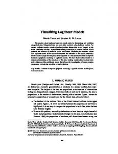
3.12.1 Equal Error Rate (EER) The equal error rate (EER) is the error rate achieved when adjusting the decision threshold such that the number of false positives and the number of false negatives are equal. This error measure is used since it is independent of the class ratio.

3.12.2 Area Under the ROC (AUC) Another popular error measure is the area under the receiver operator characteristic, or AUC for short. The receiver operator characteristic (ROC) is a curve that is drawn by plotting the true positive rate versus the false positive rate of a system for all possible decision thresholds. From this curve it can be seen directly how well a system can be tuned to achieve the desired false positive rates or true positive rates. The AUC is the integral over this curve. An example of a ROC curve is shown in Figure 3.1.

26

Chapter 4 Databases For evaluating our approach, we chose two well-established object recognition datasets: The Caltech dataset and the Pascal Visual Object Classes Challenge 2006 dataset.

4.1 Caltech The Caltech dataset1 consists of three subtasks: Airplanes, faces and motorbikes. For each class, there is a set of foreground images containing objects of the respective 1

http://www.vision.caltech.edu/html-files/archive.html

(a): airplanes

(b): faces

(c): motorbikes

(d): background

Figure 4.1. Example images from the Caltech dataset

27

Chapter 4 Databases

class

train

test

airplanes faces motorbikes

800 436 800

800 434 800

Table 4.1. Number of training and testing examples and ratio of object images vs total images in the training data for the Caltech dataset.

class, and a set of background images, mostly showing office and outdoor scenes. All images are greyscale. Table 4.1 gives an overview of the number of foreground and background images per task. Figure 4.1 shows example images from the dataset. A problem with this dataset is that the foreground images are much larger than the background images. While the foreground images have an average resolution of 700x460 pixels, the average resolution of the background images is only 200x130 pixels. As shown in [Deselaers et al., 2005a], this may lead to the undesirable effect that the classifier ’learns’ the image dimensions. So, we scale all images to a uniform height of 225 pixels, resulting in an average resolution of 340x225 pixels. The Caltech task is known to be an easy task since there is little variance in scale and rotation of the objects and since objects are always photographed from the same view point. Also, object and background images are uniformly distributed in both training and test data. Nevertheless, the Caltech dataset serves as a good baseline since it is relatively small and used extensively in the literature, so many reference results exist. The evaluation error measure for this task is the EER (Section 3.12.1).

4.2 Pascal VOC 2006 The Pascal Visual Object Classes Challenge (VOC) 2006 data [Everingham et al., 2006]2 is a more recent and more challenging dataset than the Caltech dataset. It consists of ten classes comprising man-made objects, animals and people. The VOC 2006 consisted of two tasks: Detecting the presence of an object class, and finding the bounding box of an object. While the second task would certainly be possible with an extension of our approach (cf. [Lampert et al., 2008]), we will only discuss the first task in this work. Figure 4.2 shows some example images from all classes and Table 4.2 shows the number of training and test examples for each class as well as the ratio of object images in the training data. 2

http://pascallin.ecs.soton.ac.uk/challenges/VOC/voc2006/index.html

28

4.2 Pascal VOC 2006

(a): bicycle

(b): bus

(c): car

(d): cat

(e): cow

(f ): dog

(g): horse

(h): motorbike

(i): person

(j): sheep Figure 4.2. Example images from the ten classes of the Pascal VOC 2006 dataset.

29

Chapter 4 Databases

Table 4.2. Number of training and test examples and ratio of object images vs total images in the training data for the Pascal VOC 2006 dataset.

class

train

test

object ratio

bicycle bus car cat cow dog horse motorbike person sheep

2612 2615 2595 2617 2617 2614 2617 2614 2551 2618

2676 2683 2673 2684 2686 2678 2681 2677 2608 2683

0.10 0.07 0.21 0.15 0.08 0.14 0.09 0.09 0.26 0.10

In contrast to the Caltech task there is no explicit set of background images. Instead, all images which do not concern the object of interest are used. The images from the PASCAL task are colour images with an average size of 525x420 pixels. As can be seen in Table 4.2, the training and test sets are larger, and the positive training examples only make up a small share of the training data. The images within each class have a much higher variation regarding object scale, rotation and orientation. Also, the objects may be partially occluded to some degree, making this a much more challenging task than the Caltech task. The evaluation error measure for the PASCAL VOC 2006 data is the area under the ROC (AUC) (Section 3.12.2).

30

Chapter 5 Experiments and Results In this section, we evaluate our model on the Caltech and Pascal VOC 2006 tasks. In particular we answer the questions: • How many densities are required to model the object classes without overfitting to the training data? • Which effect does regularisation (Section 3.9) have on recognition performance? • How many local features per image are needed for best recognition performance? • Which kinds of local features work best with LLMMs? • Can we achieve better recognition using second-order features? • Does falsifying training (Section 3.11) improve the results? • Does model initialisation via discriminative splitting (Section 5.3.2) work as good as the heuristic initialisation using GMDs? • How do log-linear mixture models compare to other current object recognition approaches? Since we initialise our log-linear model parameters using an equivalent GMM, we can easily compare the performances of GMMs and LLMMs: As shown in Section 3.1, LLMMs and GMMs are equivalent. This means if we initialise an LLMM with the parameters of a GMM (using the transformations from Eq. 3.19), the classification before training the LLMM will be the same.

5.1 Baseline Features In our baseline experiments, we use the following feature parameters: • Wavelet interest point detection (cf. Section 2.1.3)

31

Chapter 5 Experiments and Results

Figure 5.1. Baseline extraction points: Top row: Caltech images, bottom row: Pascal images

• 200 local features per image • appearance-based features (cf. Section 2.2.1) – Caltech: 11x11 pixels (grey), PCA reduction to to 40 dimensions – Pascal: 19x19 pixels (colour), PCA reduction to to 40 dimensions Figure 5.1 shows some examples of the feature extraction points for both databases. We use different patch sizes for the two tasks to compensate for the difference in image size. In the Caltech dataset, an image is represented by 200 patches of dimension 11x11 pixels. Assuming that the patches do not overlap, these features cover 28% of an image. When using the same patch size for the Pascal dataset, we would only capture up to 11% of an image, but with patches of dimension 19 times 19, we capture 32.7%, which is closer to the ratio on the Caltech dataset. Note, that the patches for both databases are reduced to 40 dimensions using PCA. Thus, a Caltech image is effectively reduced to 3.6%, and a Pascal image is reduced to 1.2% of its data. This reduction makes training computationally inexpensive, yet the resulting model achieves competitive performance on the Caltech task. We now present our results with the baseline setup. We evaluate models with different numbers of log-linear mixture components, i.e. different values of I in Eq. 3.23. We also examine the effect of regularisation (Section 3.9) on recognition performance. The training procedure is described in Section 3.8. In our experiments, we use a log-linear model with only first-order features, i.e. the Λ terms from Eq. 3.23 are omitted. We evaluate second-order features in Section 5.3.1.

32

5.1 Baseline Features

12

Airplanes GMD Faces GMD Motorbikes GMD Airplanes LLMM Faces LLMM Motorbikes LLMM

10

ER [%]

8

6

4

2

0 1

2

4

8

16 32 densities

64

128

256

512

Figure 5.2. Error rates for different density counts. Dotted lines: GMDs, continuous lines: LLMMs

5.1.1 Results on the Caltech Tasks For our baseline experiments we choose a fixed number of 1,500 RProp iterations. Figure 5.2 shows the error rates achieved on the Caltech database with different density counts I. Dotted lines denote the Gaussian mixture model and continuous lines denote the log-linear mixture model. We see that the LLMM generally performs better than the GMD. In particular, the LLMM achieves much better error rates with much simpler models. For example, the error rates of the LLMM with four densities are all lower than the respective GMD error rates with 512 densities, i.e. a model with 128 times more parameters. The error rate for faces is slightly above the error rates for airplanes and motorbikes since we have only approximately half the training data for this task. The increase starting at about 64 densities is clearly due to overfitting, especially when considering that the error rate on the training images is 0 for two and more densities. Table 5.1 shows how model complexity affects error rate and training time. The EER which is mostly used for evaluations on this dataset in literature is given for comparison. We see that it only slightly differs from the error rate. The table clearly shows that the LLMM can achieve acceptable recognition results using a simple model in a few minutes.

33


Table 5.1. Error rate, model complexity and training time for different numbers of densities on the Caltech airplanes task. The time value incorporates both GMD training and LLMM training, as well as data i/o and model evaluations after each training step. The tests were run on AMD Opteron processors with 2.5GHz.

# densities

# model parameters

ER

EER

training time

1 2 4 8 16 32 64 128 256 512

82 164 328 656 1,312 2,624 5,248 10,496 20,992 41,984

4.13% 2.63% 2.25% 2.38% 2.63% 2.38% 2.88% 4.13% 6.88% 7.13%

4.00% 2.75% 2.75% 2.25% 2.25% 2.50% 3.25% 4.00% 6.25% 7.25%

10min 13min 17min 35min 44min 2h 28min 3h 52min 7h 18min 15h 43min 1d 13h 0min

10

alpha=0 alpha=1e-7

8

ER [%]

6

4

2

0 0

200

400

600

800 iterations

1000

1200

1400

Figure 5.3. The effect of regularisation demonstrated on the Caltech airplanes task using an LLMM with 256 densities and a regularisation weight alpha. alpha=0 means no regularisation.

Regularisation When increasing model complexity while keeping the number of training samples constant, every classifier is prone to overfitting. This explains the ascent in error rate in Figure 5.2. A technique for avoiding overfitting of log-linear models is regularisation, introduced in Section 3.9. Figure 5.3 shows the effect of regularisation on the training process: Two models are trained on the Caltech airplanes dataset,

34


10

10

No regularization Regularization

6

6 ER [%]

8

ER [%]

8

No regularization Regularization

4

4

2

2

0 1e-08

1e-07

1e-06

1e-05

1e-04 alpha

0.001

0.01

0.1

0 1e-08

1e-07

1e-06

1e-05

1e-04 alpha

0.001

0.01

0.1

Figure 5.4. Error rates on the Caltech airplanes task for different regularisation weights alpha (red) and error rate without regularisation (green). Left: LLMM with 8 densities. Right: LLMM with 256 densities.

both with 256 densities. The graphs show the error rates on the test set after each training step. The first experiment was run without regularisation, denoted by the red graph, and the second experiment was run with regularisation, denoted by the green graph. The weighting factor used in the second experiment is 10−7 and was determined experimentally. We see that without regularisation the error rate constantly grows as the model fits to the training data. With regularisation, we first observe a peak in the error rate which then falls and reaches a constantly low level. The regularisation weight α is a sensitive parameter and needs to be chosen carefully. For each number of densities we tested 12 values for α in the range between 10−8 and 0.5. Figure 5.4 shows the error rate plotted against different regularisation values (in red) and the error rate without regularisation (in green). The left plot shows the result for a model with 8 densities, and the right plot shows the result for a model with 256 densities. We see that for the more complex model, we can achieve a significantly better error rate with regularisation (1.88%) than without regularisation (6.88%). For the simpler model, the error rate is not improved with regularisation since this model is less prone to overfitting. Also note that with regularisation, the big model outperforms the small model (1.88% vs. 2.38%). However, this comes at the cost of an almost 30 fold increase in training time. The more the model over-fits the stronger the effect of regularisation becomes. This shown in Figure 5.5. The dotted lines show the original error rates, and the continuous lines show the error rates with regularisation. For each number of densities, we choose the regularisation weight that results in the lowest error rate. For all three tasks regularisation eliminates the overfitting effect. Also, it improves the error rate for the single density models. Between two and 64 densities regularisation does not help to improve recognition.

35


10

10

Airplanes no reg Airplanes reg

6

6 ER [%]

8

ER [%]

8

Faces no reg Faces reg

4

4

2

2

0

0 1

2

4

8

16 32 densities

64

128

256

512

10

1

2

4

8

16 32 densities

64

128

256

512

Motorbikes no reg Motorbikes reg

8

ER [%]

6

4

2

0 1

2

4

8

16 32 densities

64

128

256

512

Figure 5.5. The effect of regularisation on overfitting: Error rates for different numbers of densities. Dotted lines: No regularisation, continuous lines: With regularisation, orange lines: regularisation weight.

For airplanes and motorbikes, even the ER without regularisation shows no significant improvement with more than four densities. For faces, mixture models do not show a significant improvement over a regularised single density model.

Results The principle of Occam’s razor states that model complexity should not be increased if no improvement in prediction can be achieved by doing so. Following this principle we choose four densities per class. Table 5.2 shows our baseline results on the Caltech tasks using a log-linear mixture model with four densities per class. Regularisation was not used since it does not improve the error rate at this number of densities. The respective error rates for Gaussian mixture models are given for reference. We see that we can greatly improve recognition by using log-linear mixture models.

36


80

60

50

50 ER [%]

60

50 40

40 30

30

20

20

20

10

10

10

0 2

4

8 densities

16

32

64

0 1

2

(a): bicycle 80

4

8 densities

16

32

64

1

80

50 ER [%]

60

50 ER [%]

60

40 30

30

20

20

20

10

10

8 densities

16

32

64

2

4

8 densities

16

32

64

1

50 ER [%]

60

50 ER [%]

60

50

40 30

30

20

20

20

10

10

16

32

64

64

GMD LLMM

10

0 8 densities

32

40

30

4

16

70

60

0

8 densities

80

GMD LLMM

70

40

4

(f ): dog

80

GMD LLMM

2

2

(e): cow

70

1

GMD LLMM

0 1

(d): cat 80

64

10

0 4

32

40

30

2

16

70

50

0

8 densities

80

GMD LLMM

70

40

4

(c): car

60

1

2

(b): bus GMD LLMM

70

ER [%]

40

30

1

GMD LLMM

70

60

0

ER [%]

80

GMD LLMM

70

ER [%]

ER [%]

80

GMD LLMM

70

0 1

2

(g): horse

4

8 densities

16

32

64

(h): motorbike 80

1

2

4

8 densities

16

32

64

(i): person GMD LLMM

70 60

ER [%]

50 40 30 20 10 0 1

2

4

8 densities

16

32

64

(j): sheep Figure 5.6. Error rates for different density counts. Dotted lines: GMDs, continuous lines: LLMMs

37


Table 5.2. Overview of Caltech baseline results for a log-linear mixture model with four densities per class.

Task Airplanes Faces Motorbikes

GMD ER

LLMM ER

GMD EER

LLMM EER

8.13% 8.53% 6.50%

2.25% 4.61% 2.50%

6.50% 8.30% 5.25%

2.75% 4.61% 2.75%

5.1.2 Results on the PASCAL VOC 2006 data On the PASCAL VOC 2006 dataset, we only perform experiments with up to 64 densities per class, since training on this dataset takes significantly longer than on the Caltech dataset because we have three times the amount of training data. The experiments with 1 to 16 densities showed convergence after 1,500 training iterations, while the experiments with 32 and 64 densities required 2,500 iterations to achieve convergence. Figure 5.6 shows the error rates that GMDs (dotted) and LLMMs (solid) achieve with increasing number of densities on the PASCAL tasks. Like on the Caltech data, we see that LLMMs always perform much better than GMDs. In contrast to the results on the Caltech task (Figure 5.2), however, there is often no improvement in error rate when increasing the number of densities. But as we see in Figure 5.7 the AUC increases for all subtasks when increasing the number of densities. Like on the Caltech task the biggest improvement over GMDs is achieved with a lower number of densities. The model performs best on the bus (0.90), car (0.89) and motorbike (0.89) subtasks which are all man-made objects with less variety in appearance than animals. On the other hand, animals often have less variance in colour than man-made structures. This shows that the appearance based features we use in the baseline experiments enable colour-invariant recognition. We observe the worst performance on the person task, which have high variety in appearance due to clothing. For the sake of clarity, we present further results mainly on the following three subtasks: • Cars, representing man-made structures • Persons, the most difficult task with high variety in appearance • Sheep, representing animals Saturation in the AUC starts at 32 densities per class. Considering Occam’s razor, we choose this model complexity for further experiments.

38


1

1

GMD LLMM

1

GMD LLMM

0.8

0.8

0.8

0.7

0.7

0.7

0.6

0.6

0.6

0.5

0.5 1

2

4

8 densities

16

32

64

0.5 1

2

(a): bicycle 1

4

8 densities

16

32

64

1

1

0.7

0.7

0.7

0.6

0.6

0.6

0.5 8 densities

16

32

64

2

4

8 densities

16

32

64

1

0.8

0.8

0.7

0.7

0.7

0.6

0.6

0.6

0.5 4

8 densities

16

32

8 densities

16

32

64

GMD LLMM

AUC

0.8 AUC

0.9

AUC

0.9

2

4

1

GMD LLMM

0.9

1

2

(f ): dog

1

0.5

64

GMD LLMM

(e): cow GMD LLMM

32

0.5 1

(d): cat 1

16

AUC

0.8

AUC

0.9

0.8

AUC

0.9

4

8 densities

1

GMD LLMM

0.8

0.5

4

(c): car

0.9

2

2

(b): bus GMD LLMM

1

GMD LLMM

AUC

0.9

AUC

0.9

AUC

0.9

64

0.5 1

2

(g): horse

4

8 densities

16

32

64

(h): motorbike 1

1

2

4

8 densities

16

32

64

(i): person GMD LLMM

0.9

AUC

0.8

0.7

0.6

0.5 1

2

4

8 densities

16

32

64

(j): sheep Figure 5.7. AUCs for different density counts. Dotted lines: GMDs, continuous lines: LLMMs

39


0.9

40

Car Person Sheep Car reg. Person reg. Sheep reg.

35

0.85

30 25 ER [%]

AUC

0.8

0.75

20 15

0.7 Car Person Sheep Car reg. Person reg. Sheep reg.

0.65

0.6 1

2

4

8 densities

16

32

10 5 0 64

1

2

4

8 densities

16

32

64

Figure 5.8. The effect of regularisation on the AUC (left) and error rate (right) of three Pascal VOC 2006 tasks for different numbers of densities. Dotted lines denote models trained without regularisation, continuous lines denote models with regularisation.

Regularisation Figure 5.8 shows the effect of regularisation on the error rate and AUC for different numbers of densities. In contrast to the Caltech tasks (Figure 5.5) regularisation can not improve AUC or ER for single densities. For less than 32 densities, regularisation has a slightly positive impact, but the performance with regularisation is never higher than the performance with 32 densities and no regularisation. Figure 5.9 shows the effect of different regularisation weights on the AUC. The red line shows the results of the experiments with regularisation, and the green line shows the results without regularisation. Only for 16 densities we can achieve a slight improvement over the AUC without regularisation. In the case of 1 and 64 densities, regularisation always decreases the AUC. When considering that finding the optimal regularisation parameter requires many additional training runs, regularisation does not seem to pay off on the PASCAL task. Results The results of our baseline experiments on the PASCAL VOC 2006 task are shown in Table 5.3. The ER is given for reference. Due to the class imbalance (cf. Section 4.1) the ERs have to be considered wrt. the ratio of background and object images.

5.2 Extended Features We now try to improve the baseline results on both the Caltech and PASCAL tasks by adjusting different feature parameters. Our goal is to find out which features

40

5.2 Extended Features

1

0.96

0.96

0.94

0.94

0.92

0.92

0.9

0.9

0.88

0.88

0.86

0.86

0.84

0.84

0.82

0.82

0.8 1e-08

1e-07

1e-06

1e-05 1e-04 alpha

0.001

No regularisation Regularisation

0.98

AUC

AUC

1


0.98

0.01

0.1

0.8 1e-08

1e-07

(a): 1 density

1e-06

1e-05 1e-04 alpha

0.001

0.01

0.1

(b): 16 densities

1


0.98 0.96 0.94

AUC

0.92 0.9 0.88 0.86 0.84 0.82 0.8 1e-08

1e-07

1e-06

1e-05 1e-04 alpha

0.001

0.01

0.1

(c): 64 densities Figure 5.9. AUCs on the PASCAL cars task for different regularisation weights alpha (red) and AUC without regularisation (green).

Table 5.3. Baseline results on the Pascal VOC 2006 task using an LLMM with 32 densities per class.

subtask

ER [%]


10.95 7.72 14.44 15.24 7.89 19.27 13.58 9.11 27.95 8.35

AUC 0.84 0.90 0.88 0.80 0.86 0.72 0.74 0.89 0.72 0.87

41


Table 5.4. The effect of different patch sizes on recognition performance for the Caltech task.

patch size

airplanes EER

faces EER

motorbikes EER

5x5 7x7 11x11 19x19 29x29

6.00% 1.50% 2.75% 3.00% 3.00%

10.14% 3.23% 4.61% 10.14% 13.36%

4.75% 2.00% 2.75% 2.25% 4.75%

2.25% 4.25%

5.53% 8.29%

3.25% 3.25%

5x5, 11x11, 19x19 one model separate models

work best with log-linear mixture models and to find a setup that can achieve results competitive to those found in literature.

5.2.1 Patch Size For our baseline setup, we used a fixed patch size of 11x11 for the Caltech dataset and 19x19 for the PASCAL dataset. These choices were based on reasoning and previous experiments on these datasets. We now want to experimentally determine the patch sizes that are best suited for these tasks. In our experiments, we evaluate patch sizes of 5x5, 7x7, 11x11, 19x19 and 29x29 pixels. Additionally, we examine the combination of patches of different sizes (5x5, 11x11, 19x19). For this combination two approaches are evaluated: • At each interest point, extract patches of multiple sizes and jointly perform a PCA transformation on the extracted patches. Train one combined LLMM. • Extract and PCA transform the patches separately and train an extended LLMM as presented in Section 3.7, i.e. train separate model parameters for each patch size. Either of these approaches has its strengths and weaknesses. The first approach treats patches from multiple scales as if they had the same scale. Through this we may be able to achieve (limited) scale invariance. The second approach trains one model per scale, and thus explicitly takes scale into account and models object parts of different sizes separately. When using this approach there is less training data per parameter since the number of parameters multiplies while the amount of training data stays the same. This may result in a worse model of the training data. For these feature combination approaches we use the same number of patches per image as for the experiments with single patch sizes.

42


Table 5.5. The effect of different patch sizes on recognition performance for the PASCAL task.

patch size

car AUC

person AUC

sheep AUC

3x3 5x5 7x7 11x11 19x19 29x29 5x5, 11x11, 19x19 one model sep. models

0.85 0.91 0.90 0.89 0.89 0.88

0.64 0.71 0.72 0.73 0.72 0.72

0.80 0.87 0.86 0.88 0.86 0.87

0.87 0.85

0.70 0.64

0.88 0.86

With the exception of the patch size the rest of feature and training parameters is the same as in the baseline experiments. Independent of the patch size we apply a PCA reduction to 40 dimensions1 . This means the bigger the patch size is, the higher is the information loss through projection to the 40 dimensional feature space. We deliberately made this choice in order to have the same number of model parameters in all experiments. Table 5.4 shows the results of our experiments on the Caltech tasks. We see that 7x7 pixel patches yield the best results on all three tasks. Combining patches of different dimensions does not lead to better results than with 7x7 pixel patches. On the airplanes and faces tasks the combined approach of feature combination works better than the separate approach because faces and airplanes appear in different scales. On the motorbikes task, both approaches work equally well because all motorbikes in the dataset have approximately the same size, so a scale invariant model does not have an advantage. The results on the PASCAL dataset are shown in Table 5.5. For the person and sheep subtasks we achieve the best result with 11x11 pixel patches. On cars, 5x5 pixel patches perform best. Like on the Caltech task, the feature combination using one model works better than the approach with separate models due to the high variance in object scale. Neither achieves a better performance than a single size model. For future experiments, we choose a patch size of 7x7 for the Caltech task and 11x11 for the PASCAL task. 1

We do not use PCA for the 5x5 pixel patches extracted from the greyscale Caltech images since the feature dimensionality is only 25.

43


Table 5.6. Training times for different numbers of local features per class and different model complexities on the Caltech airplanes and PASCAL car tasks. The training times of the other tasks of the respective datasets are similar. The time format in hours:minutes:seconds. Experiments were performed on 2.8GHz AMD Opteron machines. (a): Caltech airplanes

100 200 500 1000

LF LF LF LF

1 dens.

2 dens.

4 dens.

8 dens.

0:06:49 0:11:32 0:23:57 0:39:17

0:09:03 0:22:53 0:46:41 1:00:17

0:15:26 0:38:12 1:00:10 1:44:31

0:29:00 1:08:06 1:46:35 2:11:03

(b): PASCAL car

100 200 500 1000

LF LF LF LF

1 dens.

2 dens.

4 dens.

8 dens.

16 dens.

32 dens.

64 dens.

0:26:12 0:50:36 1:49:33 3:12:46

0:42:21 1:16:31 2:11:06 5:34:00

0:56:58 2:14:16 3:43:57 9:23:03

1:51:56 3:32:41 9:17:24 15:14:54

3:40:56 6:26:33 15:38:06 28:31:00

5:16:36 12:20:27 23:23:15 55:22:00

13:26:56 18:44:14 67:47:00 125:00:00

5.2.2 Number of Local Features per Image We now want to determine how many patches we need to extract per image to optimally discriminate object from background. Because this parameter affects the amount of training data, we also need to find the optimal model size for each number of patches per image. So, we evaluate our model using 100, 200, 500 and 1,000 patches per image and a model size of 1-16 or 1-64 densities per class for the Caltech and PASCAL tasks respectively. The maximum number of local features (LFs) we extract per image when using an interest point detector depends on the contents of the image. We choose the maximum value of 1,000 patches for Caltech because on 95% of the Caltech images more than 1,000 wavelet interest points are detected. 99% of the Caltech images have more than 500 interest points. On the PASCAL tasks experiments with up to 4,000 LFs were performed. On 99.9% of the images over 1,000 interest points were detected, 95% of the images have over 2,000 interest points and 81% still have over 4,000 interest points. The typical memory usage of the training process with 1,000 LFs per image is 400MB on Caltech and 2GB on PASCAL. These values scale linearly with the amount of training data. The training times for two typical tasks of the two datasets are shown in Table 5.6. We see that depending on the amount of data and the

44


Table 5.7. EER for different numbers of local features and densities on the three Caltech tasks. (a): airplanes

100 200 500 1000

LF LF LF LF

1 dens.

2 dens.

4 dens.

8 dens.

2.0% 2.0% 1.5% 1.75%

2.0% 1.25% 1.5% 1.75%

1.75% 1.5% 2.0% 1.75%

1.5% 1.75% 2.25% 1.25%

(b): faces

100 200 500 1000

LF LF LF LF

1 dens.

2 dens.

4 dens.

8 dens.

3.23% 5.53% 3.69% 5.53%

4.15% 3.69% 4.15% 4.61%

3.23% 3.23% 3.69% 3.69%

3.23% 3.69% 5.53% 4.61%

(c): motorbikes

100 200 500 1000

LF LF LF LF

1 dens.

2 dens.

4 dens.

8 dens.

3.5% 2.5% 2.5% 2.75%

2.25% 3.0% 2.25% 2.25%

2.25% 2.0% 2.25% 1.75%

2.0% 2.0% 2.25% 1.75%

complexity of the model, times are in the range from 7 minutes to 2 hours on Caltech and from 26 minutes to more than a day on PASCAL. Training complexity is linear in both number of training samples and number of densities per class. Depending on the possible applications of LLMMs in object recognition, training time is an important criterion for choosing model and feature parameters. In cases where the training data changes frequently and limited computing power is available, a more resource friendly setup is preferable and tradeoffs in recognition accuracy will be made. The results for the Caltech task are shown in Table 5.7, and the results for the PASCAL VOC 2006 tasks car, person, and sheep are shown in Table 5.8. Surprisingly, using more features does not help always. For example, we achieve an EER of 3.23% on the Caltech faces task using 100 LFs per image, and only up to 3.69% with 1,000 LFs per image. On the PASCAL car task, we achieve an AUC of 0.9 with 100 features, but only 0.84 with 4,000 features. This is in contrast to

45


Table 5.8. AUC for different numbers of local features and densities on PASCAL tasks car, person and sheep. (a): car

100 200 500 1000 2000 4000

LF LF LF LF LF LF

1 dens.

2 dens.

4 dens.

8 dens.

16 dens.

32 dens.

64 dens.

0.86 0.87 0.86 0.84 0.82 0.8

0.88 0.88 0.88 0.86 0.81 0.81

0.86 0.85 0.85 0.83 0.8 0.81

0.84 0.86 0.85 0.86 0.83 0.81

0.87 0.87 0.87 0.86 0.85 0.82

0.89 0.89 0.88 0.85 0.83 0.83

0.9 0.89 0.87 0.86 0.84 0.84

(b): person

100 200 500 1000 2000 4000

LF LF LF LF LF LF

1 dens.

2 dens.

4 dens.

8 dens.

16 dens.

32 dens.

64 dens.

0.71 0.7 0.7 0.67 0.66 0.64

0.72 0.72 0.71 0.66 0.62 0.64

0.7 0.72 0.71 0.68 0.68 0.65

0.67 0.66 0.69 0.65 0.69 0.66

0.69 0.69 0.7 0.66 0.66 0.67

0.7 0.71 0.72 0.71 0.69 0.67

0.73 0.73 0.72 0.71 0.7 0.68

(c): sheep

100 200 500 1000 2000 4000

LF LF LF LF LF LF

1 dens.

2 dens.

4 dens.

8 dens.

16 dens.

32 dens.

64 dens.

0.81 0.82 0.82 0.81 0.8 0.78

0.86 0.87 0.86 0.86 0.83 0.82

0.84 0.81 0.85 0.86 0.86 0.85

0.83 0.84 0.85 0.84 0.83 0.81

0.86 0.85 0.87 0.88 0.85 0.85

0.85 0.87 0.86 0.86 0.86 0.85

0.87 0.88 0.86 0.87 0.87 0.85

[Nowak et al., 2006b] who found that more features can always improve performance when using a bag of visual words approach similar to [Deselaers et al., 2005a]. This does not appear to be the case for LLMMs. An explanation for this behaviour is that the interest point detector returns the interest points sorted by saliency. That is, in our experiments with 100 LFs, we use the 100 most salient points of the image. When increasing the number of LFs we add points with lower saliency that might not add any new information to the

46


5

Airplanes Faces Motorbikes

EER [%]

4

3

2

1

0 100

200

300

400 500 600 700 Local features per image

800

900

1000

Figure 5.10. The best EER (over all density counts) for each number of local features on the Caltech tasks

0.95

Car Person Sheep

0.9

AUC

0.85

0.8

0.75

0.7

0.65 500

1000

1500 2000 2500 3000 Local features per image

3500

4000

Figure 5.11. The best AUC (over all density counts) for each number of local features on the PASCAL tasks

model. Additional points might even disturb the model because they add noise. On the Caltech motorbikes task however, the EER decreases the more data we add. The reason is that nearly all motorbikes in this dataset are shot in front of a white background, causing all interest points to lie on a motorcycle. Therefore, no background clutter is added to the model of the object class when increasing the number of LFs and motorbikes can be modelled more and more accurately. There are two minima on the Caltech airplanes task: 1.25% are achieved using 2 densities and 200 LFs as well as with 8 densities and 1,000 LFs. Here we would

47


decide on the former setup since the model is four times simpler and we only need 1 5 th of the training data, and training is more than five times faster (23 min. vs. 131 min.) On the three PASCAL tasks we examine, 64 densities per class generally perform best, and an increase in the number of LFs does not yield significant improvements, and sometimes even decreases the AUC. In order to find the optimal number of LFs per image, we choose the number of densities that yields the best result for each number of LFs. Figure 5.10 shows the resulting EERs for the Caltech tasks and Figure 5.11 shows the AUCs on the PASCAL tasks. On the Caltech faces and motorbikes tasks, the best EERs are the same for 100 and 200 LFs per image. On the airplanes task, the result improves with LFs. When increasing the feature count to 500, we always observe an increase in EER, and when doubling the feature count again, there are slight increases for airplanes and motorbikes, but only for motorbikes, the EER with 1,000 LFs (1.75%) is lower than the EER with 200 LFs (2.0%). However, this increase is not big enough to justify the five fold increase of training data. For the Caltech tasks we therefore keep the amount of 200 LFs per class from the baseline setup. On the PASCAL tasks, the AUC constantly decreases for more than 200 LFs except for the sheep task where the first maximum is again reached with 1,000 LFs per image. So, on the three PASCAL tasks we observe, 200 LFs per image clearly are the optimal choice.

5.2.3 Types of Local Features In Chapter 2 methods for determining extraction points and descriptors for local features were introduced. In the previous experiments in this chapter, only appearance-based features from wavelet extraction points were used. We now examine how well other interest points and descriptors are suited for object recognition with LLMMs and if the combination of different feature types can improve the results. The extraction methods we examine are: Appearance based features extracted at wavelet points (“Wave”), DoG points, Random points (“Rand”), and grid points, SIFT interest points and descriptors and patch histograms extracted at random points (“Hist”). For the appearance based features the patch dimensions found to be optimal in the previous sections are used: 7x7 pixels for the Caltech tasks and 11x11 pixels for the PASCAL tasks. 200 local features of each type are extracted, except for the grid points that are extracted from a 14x14 grid yielding 196 points. The patch histograms are extracted at random points with an extraction size of 23x23 pixels. Grey histograms with eight bins were extracted from the Caltech images, and colour histograms with four bins per dimension, yielding a total of 64

48


Table 5.9. The performance (in EER) of different types of local features on the Caltech dataset.

airplanes Wave DoG Rand Grid SIFT Grey hist

1.5% 3.5% 1.75% 2.75% 6.25% 10.0%

faces 3.23% 7.37% 2.77% 3.23% 18.89% 23.5%

motorbikes 2.0% 4.75% 4.0% 3.5% 7.25% 9.75%

Table 5.10. The performance (in AUC) of different types of local features on the PASCAL dataset.

Wave DoG Rand Grid SIFT Colour hist

car

person

sheep

0.89 0.88 0.89 0.86 0.87 0.75

0.73 0.69 0.67 0.64 0.65 0.62

0.88 0.89 0.86 0.88 0.81 0.84

bins, were extracted from the PASCAL images. The results on the Caltech tasks are shown in Table 5.9 and the results on the PASCAL tasks are shown in Table 5.10. More intense colours denote better results. Despite their simplicity appearance based features perform best. The best performing interest points are wavelet points. DoG points perform rather bad on the Caltech tasks, but well on the PASCAL tasks. Random points have a slight advantage over grid points, though this may also be noise. We expected a better performance from the SIFT descriptors, which are specially tailored towards robust object recognition, but they are among the worst performing features together with grey and colour histograms. This contradicts with the findings of Mikolajczyk and Schmid [2005] who evaluated different descriptors wrt. their robustness to scale, orientation, lighting and various other properties and found SIFT to perform best on nearly all tasks. On the Caltech airplanes task wavelet interest points perform much better than DoG points, and random points perform nearly as good as wavelet points. As shown in Figure 2.3 wavelet points tend to be more spread across the image while DoG points focus around areas of high contrast. Wavelet and random points perform better on the airplanes task, since most pictures in the airplanes dataset depict flying airplanes. Because the sky is relatively homogeneous, the interest points,

49


Figure 5.12. Interest point detectors on Caltech faces: Most DoG interest points (left) are detected in the background, wavelet features (right) cover both face and background.

and especially the DoG points, focus on the object so that the sky which can serve as an important cue for recognition is underrepresented in the model. The scale independence of DoG points does not bring an advantage here since the airplanes have relatively little variation in size. On the Caltech faces task random points perform best, and grid and wavelet points do slightly worse. DoG points have over twice the EER of wavelet points. We expected that an interest point detector that can robustly detect facial features would have a clear advantage over methods that do not use image contents. A possible explanation for this can be found in [Nowak et al., 2006a] who found that random points can outperform interest points in many settings. Figure 5.12 shows why interest point detectors are not ideal for this task. Because the faces are photographed in offices or outdoors and thus have a feature-rich background, interest point detectors, especially DoG, mostly sample the background and cover little of the face itself. A specialised approach that utilises face detection techniques would have an advantage on this task. On the PASCAL car and sheep tasks appearance based features perform well regardless of the type of interest points. This is because both object classes have typical backgrounds (street scenes for cars and grasslands for sheep) that help in the classification. It was expected that an interest point detector that robustly detects class-specific features would help the classification, but this is not the case. Like on the Caltech faces task DoG points perform worse than wavelet points on the PASCAL person task. In contrast to the Caltech faces task random and grid points perform worse than wavelet points because in the PASCAL dataset persons usually take up much less image space than on Caltech and thus less random points lie on the persons.

50


Table 5.11. Different combinations of local features on the Caltech dataset (EER%). (a): Combinations of extraction points

Wavelet

Grid

Random

Airplanes

Faces

Motorbikes

X X X

1.5 1.75 2.75 3.0 2.0 1.25 1.75

3.23 2.77 3.23 3.69 3.69 1.84 5.53

2.0 4.0 3.5 2.5 2.25 2.75 2.5

X X X X X X

X X

X

(b): Combinations of descriptors

Appearance

SIFT

Histograms

X X X X X X

X X

X X X X

1.5 6.25 10.0 3.0 1.75 2.25 3.25

3.23 18.89 23.5 11.52 4.61 5.99 5.07

2.0 7.25 9.75 5.25 2.5 1.0 1.5

Feature Combinations In the following we examine different combinations of extraction points and and compare their performance to the the individual features presented before. For this we use the extended LLMM introduced in Section 3.7. In the experiments we combine: • Different extraction points: Wavelet, grid (on Caltech), DoG (on PASCAL) and random points, using appearance based features • Different descriptors: Appearance (at wavelet points), SIFT (at DoG points with SIFT extensions) and histograms (at random points) We choose the three best performing extraction points for both datasets, so we use grid points on the Caltech dataset and DoG points on the PASCAL dataset. Our experiments include all subsets of both combinations. The results on the Caltech tasks are shown in Table 5.11 and the results on the PASCAL tasks are shown in Table 5.12. For reference the individual features are included in the tables as well.

51


Table 5.12. Different combinations of local features on the PASCAL dataset (AUC). (a): Combinations of extraction points

Wavelet

DoG

Random

Car

Person

Sheep

X X X

0.89 0.88 0.89 0.9 0.92 0.9 0.91

0.73 0.69 0.67 0.72 0.73 0.75 0.76

0.88 0.89 0.86 0.9 0.91 0.89 0.91

X X X X X X

X X

X

(b): Combinations of descriptors

Appearance

SIFT

Histograms

X X X X X X

X X

X X X X

0.89 0.87 0.75 0.86 0.85 0.92 0.88

0.73 0.65 0.62 0.71 0.7 0.74 0.72

0.88 0.81 0.84 0.83 0.85 0.87 0.84

In most cases feature combinations perform better than individual features. The improvements are remarkable: on the Caltech faces task the best EER with a single type of extraction points is improved by 33% relative through combinations. The combination of wavelet and grid points strongly improves the result on the Caltech airplanes and faces tasks. The AUC achieved on the PASCAL car, person, and sheep tasks is consistently improved by 0.03 using combined extraction points. On the PASCAL car and sheep tasks the combination of wavelet and random points outperforms all individual interest points by at least 0.02 in AUC. When combining all three types of points the AUC on the person task rises from 0.73, using only appearance-based descriptors, to 0.76 which is the best result on this task. The combination of different feature types leads to improvements on the Caltech motorbikes task: the combination of SIFT and appearance based features achieves half of the EER than of appearance based features alone. On the PASCAL cars task this combination improves the result of appearance based features by 0.03 AUC. The results show that combinations of different interest points and descriptors

52

5.3 Variations in training

Table 5.13. Results achieved on the Caltech dataset (left) and the PASCAL dataset (right) when including absolute spatial information in the LLMM

EER %

Baseline

Spatial

AUC

Baseline

Spatial


2.75% 4.61% 2.75%

1.50% 2.77% 1.00%

car person sheep

0.88 0.72 0.87

0.88 0.68 0.86

can capture more image information and thus help in the modelling of the object classes. This shows in clearly improved recognition performance.

5.2.4 Absolute Spatial Information The model extension introduced in Section 3.6 allows to use the absolute positions of local features in images as a cue for object recognition. Naturally this only helps to improve the performance of our system if objects are at roughly the same position. Therefore, we expect improvements on the Caltech dataset but not on the PASCAL dataset. Table 5.13 shows the results achieved on the Caltech and PASCAL datasets. Baseline results are given for comparison. As expected, the results on PASCAL cannot be improved by absolute position information since the objects can be arbitrarily positioned in the images. On the Caltech tasks absolute position information brings a remarkable improvement in recognition performance. Even for the airplanes and faces tasks where the object positions slightly vary the impact is clearly recognisable.

5.3 Variations in training In the previous section we investigated which and how much training data is best suited for object recognition with LLMMs. While the input data was varied, the model and training procedure were mostly kept fixed. Now, we investigate how different parameters for model and training affect the performance. In the following experiments the baseline setups presented in Section 5.1 are used.

5.3.1 Second-order Features So far only first-order features were used i.e. the Λ term in Eq. 3.23 was omitted since it squares the amount of parameters and thus the time needed for training. Now, we consider the full second-order models.

53


1st order train 1st order test 2nd order train 2nd order test

14 12

ER [%]

10 8 6 4 2 0 0

100

200

Iteration

300

400

500

Figure 5.13. Comparison of the progression of the train and test error rate of first and second-order models. Depicted: Caltech faces task, baseline features, 8 densities per class.

Because of the increased amount of parameters second-order models are more prone to overfitting than first-order models if insufficient training data is given. This can be seen in Figure 5.13 that shows the progression of the train and test ER of a first-order model (red) and a second-order model (green) on the Caltech faces task that has only 436 training images. Both models have eight densities per class and are initialised using a Gaussian mixture model. To initialise the first-order model the covariances of the GMD are pooled (cf. Section 3.3). The initial error rate of the second-order model is higher since the unpooled GMD that it is initialised with is more prone to overfitting than the pooled one that we initialise the firstorder model with. The second-order model adjusts to the data much faster than the first-order model resulting in a much steeper initial phase that can be observed on both training and test data. After about 30 iterations, the train error rate of both models is 0. The test error rate of the second-order model starts rising while the error rate of the first-order model continues to decline. This effect can be avoided by either using a second-order model with less densities or by using regularisation. Next, we consider the progression of the error rate of a second-order model during training on a PASCAL task (Figure 5.14). Here, the test error rate remains constant. Because for the PASCAL tasks three times the training data is available overfitting is not as strong as on the Caltech tasks even with a more complex model. In the following we examine the performance of second-order LLMMs with different numbers of densities and different regularisation weights. Figure 5.15 shows the comparison of first and second-order models on the Caltech dataset. The second-order models consistently perform worse than the first-order models due to overfitting. The EERs of the second-order experiments vary more

54


1st order train 1st order test 2nd order train 2nd order test

14 12

ER [%]

10 8 6 4 2 0 0

100

200

Iteration

300

400

500

Figure 5.14. Comparison of the progression of the test error rate of first and second-order models. Depicted: Pascal sheep task, baseline features, 16 densities per class.

12

Airplanes 1st Faces 1st Motorbikes 1st Airplanes 2nd Faces 2nd Motorbikes 2nd

10

EER [%]

8

6

4

2

0 1

2

4

densities

8

16

32

Figure 5.15. First-order models vs. second-order models on the Caltech dataset.

strongly since they have less training data per model parameter which makes the models less stable. The comparison of first and second-order models on the PASCAL task is shown in Figure 5.16. The plot shows the AUC for different numbers of densities. In contrast to the Caltech tasks second-order models perform better than first-order models with the exception of single density models. Clear and consistent improvements can be observed. For example, the AUC on sheep with four densities per class improves from 0.83 to 0.88 and the AUC on person with 32 densities improves from 0.7 to 0.77. On the car and sheep tasks the strongest improvement is observed

55


1

Car 1st Person 1st Sheep 1st Car 2nd Person 2nd Sheep 2nd

0.95

AUC

0.9 0.85 0.8 0.75 0.7 1

2

4

densities

8

16

32

Figure 5.16. First-order models vs. second-order models on the Pascal dataset.

12

Airplanes no reg Faces no reg Motorbikes no reg Airplanes reg Faces reg Motorbikes reg

10

EER [%]

8

6

4

2

0 1

2

4

densities

8

16

32

Figure 5.17. The effect of regularisation on the EER of second-order LLMMs on the Caltech task.

between four and eight densities. Less improvement is observed for higher density counts. On the person task the improvement increases with more densities which was expected due to the high difficulty of the task. Regularisation In Section 5.1.1 we found that regularisation can improve the results of first-order models that are prone to overfitting. We thus expect improvements for second-order models that show strong overfitting behaviour on the Caltech tasks. Figure 5.17 shows that improvements can indeed be achieved but that they differ from task

56


1

Car no reg Person no reg Sheep no reg Car reg Person reg Sheep reg

0.95 0.9

AUC

0.85 0.8 0.75 0.7 0.65 1

2

4

densities

8

16

32

Figure 5.18. The effect of regularisation on the AUC of second-order LLMMs on the PASCAL task.

Table 5.14. Comparison of the best results, model complexity and training time of first and second-order models on the PASCAL tasks.

first-order

car person sheep

second-order

densities

params.

time

AUC

densities

params.

time

AUC

64 128 128

5248 10,496 10,496

41h 51h 52h

0.90 0.75 0.88

32 32 2

105,024 105,024 6,654

85h 77h 7h

0.90 0.77 0.88

to task. On the motorbikes task, there is a consistent improvement of about one percent for all density counts except single densities. On the airplanes task the only improvement is achieved with four densities, and the EER of faces only improves for one and eight densities. But even with regularisation the EERs are much worse than the EERs achieved by first-order models. This is because the Caltech training data is insufficient for training second-order models. On the PASCAL tasks there is less overfitting, so fewer improvements through regularisation are expected. Figure 5.18 shows that there are in fact hardly improvements for the car and person tasks for more than four densities. With less densities the AUC is improved such that the regularisation graph is nearly a flat line for both tasks with the exception of a slight improvement on the car task with 32 densities. On the person subtask there is a consistent increase in AUC for eight and less densities, making the overall graph flatter as well. This suggests that when second-order features are used and regularisation is properly tuned, mixture models have little advantage over single density log-linear models.

57


Table 5.14 gives a pragmatic comparison of first and second-order models. This table shows the best AUC achieved for each class with first and second-order models with regularisation. For a direct comparison model complexity and training times are given. In general, second-order models lead to slight improvements at much higher computational cost. The sheep class appears to be a remarkable exception, since the same AUC can be achieved in a seventh of the time using a simpler secondorder model. It should be noted though that an only slightly worse AUC of 0.87 can be achieved with a first-order model with 8 densities in only 4 hours.

5.3.2 Discriminative Splitting Since the training of LLMMs is a non-convex optimisation problem, the initialisation of the model plays an important role. Experiments with random initial LLMM parameters showed that without initialisation training does not work well on the model. Naturally, a random model achieves an error rate of approximately 50% (given uniform class distribution, on the Caltech tasks). Training the model slightly changes the parameters but does not affect the decisions and the error rate at all. In previous experiments, the LLMMs were initialised with GMDs trained using the EM algorithm (cf. Section 3.3). This initialisation works in practice but makes the training process inconsistent since the training of a GMD is generative while the training of an LLMM is discriminative. An approach for a discriminative initialisation of LLMMs is discriminative splitting, presented in Section 3.10. An important parameter for discriminative splitting is the number of training iterations to perform between two splits. We examine two approaches: 1. 10 training iterations between splits: In the splitting phase the model parameters are only slightly changed and the model is trained to convergence once the desired number of densities exists. 2. 500 training iterations between splits: After each split the model is trained until convergence. Experiments were performed on both the Caltech and the PASCAL tasks using the optimal number of splits determined in Section 5.1: 2 splits on the Caltech tasks and 5 splits on the PASCAL tasks. Figure 5.19 shows the development of the AUC on the PASCAL cars task for both training approaches. The AUCs on both training and testing data are given. When using approach 1 (top), the training and testing AUCs generally rise during the splitting phase with slight drops caused by the disturbance of the model parameters after splitting. After the splitting, the test AUC rapidly decreases due to overfitting, while the training AUC rises rapidly and reaches 1.0 after 300 iterations. After

58


1

PASCAL car test PASCAL car train

0.98

0.96

0.96

0.94

0.94

0.92

0.92 AUC

AUC

1

PASCAL car test PASCAL car train Splits

0.98

0.9

0.9

0.88

0.88

0.86

0.86

0.84

0.84

0.82

0.82

0.8

0.8 10

20

30 Iteration

40

50

0

500

1000

1500 Iteration

2000

2500

(a): Splitting every 10 iterations for 50 iterations. Left: Closeup of the first 60 iterations. Right: Full view of 2550 iterations. 1

PASCAL car test PASCAL car train Splits

0.98 0.96 0.94

AUC

0.92 0.9 0.88 0.86 0.84 0.82 0.8 500

1000

1500 Iteration

2000

2500

(b): Splitting every 500 iterations for 2500 iterations. Figure 5.19. The development of the AUC when training an LLMM with discriminative splitting. Task: PASCAL cars

reaching its minimum the testing AUC slowly rises but does not reach its optimum again. When using approach 2 both the training and testing AUCs increase after the first split, but with every following split the training AUC rises while the testing AUC declines. After the desired number of five splits the testing AUC slowly rises but does not reach the optimum again after 3,000 iterations. We now compare the training of the two discriminative splitting approaches to the training of a model initialised using a GMD that has the same number of densities as the final splitted models (Figure 5.20). On the PASCAL task cars the best AUC is achieved when initialising the LLMM with a GMD. The two discriminative splitting approaches achieve approximately the same maximum, but approach 1 arrives at the maximum earlier. Overall, using GMD initialisation is favourable

59


0.9

8

GMD initialisation 5 * 10 iters 5 * 500 iters

0.89

GMD initialisation 5 * 10 iters 5 * 500 iters

7

0.88 0.87

6 EER

AUC

0.86 0.85

5

0.84 0.83

4

0.82 0.81

3

0.8 0

500

1000 1500 Iteration

2000

2500

0

200

(a): PASCAL car

400

600

800 Iteration

1000

1200

1400

(b): Caltech faces

Figure 5.20. The development of the AUC/EER for GMD initialisation versus the two different discriminative splitting approaches.

Table 5.15. Comparison of GMD initialisation and discriminative splitting on the Caltech and PASCAL tasks. The results for discriminative splitting are the minima/maxima of all EERs/AUCs achieved in training. (a): Caltech

Airplanes Faces Motorbikes

GMD

Splitting 1 opt

Splitting 2 opt

2.75% 4.61% 2.75%

2.75% 2.77% 2.50%

2.50% 4.61% 3.00%

(b): PASCAL

Car Person Sheep

GMD

Splitting 1 opt

Splitting 2 opt

0.90 0.71 0.88

0.87 0.71 0.87

0.87 0.71 0.87

since it achieves much better results. On the Caltech faces task the best EER of 2.8% is achieved using the first splitting approach shortly after the second split. The model initialised with a GMD achieves a slightly worse optimum of 3.2% at the same iteration. Then, its EER rises due to overfitting. Splitting approach 1 achieves the better optimum. Still, GMD initialisation is favourable since it shows the most stable behaviour and achieves approximately the same minimum equally fast as the first splitting approach.

60


Table 5.15 shows a comparison of the results achieved with GMD initialisation to the best results achieved during training with the two splitting approaches. On the Caltech task where only two splits were made, the results for GMD initialisation and splitting are similar. On the faces task the first splitting approach achieves a clearly better EER than the two other approaches but as shown in Figure 5.20 the minimum EER achieved with GMD initialisation is similar. On PASCAL, the results obtained with GMD initialisation are all equally good or better than the results achieved with splitting. Models initialised by splitting are more prone to overfitting. This can likely be avoided using regularisation. Splitting approach 1 was found to be favourable over splitting approach 2 since it achieves results equal or better than approach 2 within less training iterations. On the Caltech task where only two splits were performed results are comparable to results with GMD initialisation, but on PASCAL where five splits were found to be optimal GMD initialisation performs clearly better. The conclusion that splitting only works for initialising models with few densities is backed by the decrease in performance of approach 2 after two or more splits. An advantage of splitting is that it can achieve good results faster, but for density counts higher than 2 GMD outperforms splitting.

5.3.3 Falsifying Training Falsifying training (cf. Section 3.11) has two parameters: The percentage of the training data that is selected in the falsification step and the number of iterations between these steps. We perform experiments with percentages of 12.5%, 25%, 50%, and 75% and iteration counts of 1, 10, 50, 100, and 500. Table 5.16 shows the results on the Caltech dataset and Table 5.17 shows the results on the PASCAL dataset. The respective results without falsifying training are given for comparison. It can be seen that performance decreases with an increasing number of iterations between falsification steps. This is because the more iterations are performed between falsifying steps, the more the model fits to the selected percentage of the training data, thus misclassifying the images that it had classified correctly before. It thus seems optimal to exchange the training data in every step. We further observe that the results improve when increasing the percentage of selected images from 12.5% to 50%. The explanation for this is that the less training data we select, the higher the specialisation to this part of the data gets and the worse the overall performance becomes. This results in an oscillation effect shown in Figure 5.212 . 2

Interestingly, the plot resembles the ECG of a heart attack patient. The author hopes that this is a coincidence

61


Table 5.16. The effect of different falsifying training parameters on the performance on the Caltech dataset. Columns: Percentage of data in each falsifying step. Rows: Iterations between falsifying steps. (a): airplanes, normal tr.: 2.50% EER

iters

12.5%

25%

50%

75%

1 10 50 100 500

3.0% 6.0% 3.5% 9.5% 41.25%

2.75% 2.25% 7.25% 8.75% 4.75%

2.25% 2.25% 3.5% 20.75% 2.25%

2.25% 2.0% 2.5% 2.25% 2.75%

(b): faces, normal tr.: 5.53% EER

iters

12.5%

25%

50%

75%

1 10 50 100 500

4.15% 4.15% 4.61% 11.06% 23.04%

4.15% 4.15% 7.37% 8.29% 21.2%

4.15% 4.61% 6.91% 4.15% 22.58%

5.07% 4.15% 4.15% 5.07% 4.61%

(c): motorbikes, normal tr.: 3.75% EER

iters

12.5%

25%

50%

75%

1 10 50 100 500

2.5% 3.25% 4.0% 3.25% 9.5%

2.5% 2.75% 3.5% 3.5% 4.5%

2.5% 2.75% 2.0% 2.25% 3.0%

2.5% 3.0% 2.5% 2.75% 2.5%

Considering the experiments where training data was exchanged in every step on Caltech, no improvement is observed when increasing the selected percentage from 50% to 75%, so 50% is a good choice. A positive side effect of falsifying training is that training is faster because we use less training data per iteration. Falsifying training improves the results on relatively simple datasets such as Caltech where the hardest training examples still help improve the model. The PASCAL dataset contains images where the object is depicted very small or partially occluded. When only these images are selected as training data recognition becomes worse. Because of this falsifying training has no positive effect on recognition on the PASCAL tasks.

62

5.4 Results and Conclusion

Table 5.17. The effect of different falsifying training parameters on the performance on the PASCAL dataset. Columns: Percentage of data in each falsifying step. Rows: Iterations between falsifying steps (a): car, normal tr. 0.89 AUC

iters

12.5%

25%

50%

75%

1 10 50 100 500

0.84 0.6 0.68 0.38 0.77

0.89 0.88 0.88 0.88 0.88

0.89 0.88 0.88 0.89 0.89

0.89 0.88 0.89 0.88 0.88

(b): person, normal tr. 0.72 AUC

iters

12.5%

25%

50%

75%

1 10 50 100 500

0.66 0.48 0.61 0.43 0.45

0.69 0.51 0.62 0.41 0.64

0.72 0.72 0.72 0.73 0.73

0.72 0.72 0.72 0.73 0.73

(c): sheep, normal tr. 0.86 AUC

iters

12.5%

25%

50%

75%

1 10 50 100 500

0.86 0.88 0.84 0.73 0.79

0.86 0.87 0.86 0.87 0.86

0.86 0.87 0.87 0.86 0.86

0.86 0.87 0.87 0.86 0.86


In this chapter we have examined the effect of several feature and model parameters on the recognition performance. We now summarise the key findings and present results that are based on these findings. We also compare these results with other approaches from the literature.

63


100 iterations, 50 percent GMD init

14 12

ER [%]

10 8 6 4 2 0 0

200

400

600

800 Iteration

1000

1200

1400

1600

Figure 5.21. An example where the wrong choice of parameters leads to error rate oscillation (red). The progression of the error rate during normal training (green) is given for comparison. Task: Caltech faces.

Table 5.18. Results on the Caltech tasks using the final setup.

task

2 dens.

4 dens.

8 dens.

baseline


2.25% 2.30% 1.25%

2.00% 5.99% 0.75%

1.75% 5.53% 1.25%

2.75% 4.61% 2.75%

Table 5.19. Results on the PASCAL tasks using the final setup.

64

task

16 dens.

32 dens.

64 dens.

baseline


0.88 0.95 0.91 0.84 0.89 0.78 0.80 0.92 0.75 0.90

0.87 0.94 0.92 0.86 0.88 0.77 0.82 0.90 0.76 0.89

0.88 0.95 0.91 0.84 0.85 0.79 0.79 0.90 0.74 0.90

0.83 0.90 0.88 0.80 0.86 0.72 0.74 0.89 0.72 0.87


Table 5.20. The tuned setups for the Caltech and PASCAL datasets.

Model complexity Falsifying training Regularisation LFs per image and LF type Patch size Feature types

Absolute spatial information

Caltech

PASCAL

2 – 8 densities 50% each iteration yes 200 7x7 pixels patches at wavelet and grid points, SIFT

32 – 128 densities no no 200 11x11 pixels patches at wavelet, DoG, and random, points, SIFT no

yes

5.4.1 Conclusion Having investigated the questions at the beginning of this chapter we are now able to provide answers: • How many densities are required to model the object classes without overfitting to the training data? This depends on the amount of training images and local features extracted. For the Caltech dataset that has 436-800 training images per task, 4 densities have turned out to be optimal. For the PASCAL VOC 2006 dataset that has about 2,600 training images per task, 32 densities per class are the best choice. We extracted 200 LFs per image. For higher numbers of local features more complex models are necessary. • Which effect does regularisation (Section 3.9) have on recognition performance? We have found that regularisation helps to avoid overfitting if the number of model parameters is too high for the given amount of training data. However, the performance of a too complex model with regularisation is not much better than the performance of an unregularised model with suitable complexity. • How many local features per image are needed for best recognition performance? Contrary to results with other methods [Nowak et al., 2006a] our experiments have clearly showed that 200 local features per image are optimal for most of the Caltech and PASCAL tasks.

65


Table 5.21. Comparison of the results of LLMMs on the Caltech task with other approaches.

approach

airplanes

faces

motorbikes

LLMMs baseline LLMMs improved features LLMMs with spatial positions LLMMs second-order LLMMs disc. splitting LLMMs falsifying training LLMMs combined

2.75% 1.25% 1.50% 5.00% 2.75% 2.25% 1.75%

4.61% 1.84% 2.77% 8.29% 2.77% 4.15% 2.30%

2.75% 1.00% 1.00% 4.00% 2.50% 2.50% 0.75%

GMDs [Hegerath et al., 2006] spatial GMDs [Hegerath et al., 2006] discr. spatial GMDs [Hegerath et al., 2006] discr. BoVW [Deselaers et al., 2005a] Statistical model [Fergus et al., 2003] Texture features [Deselaers et al., 2004] Segmentation [Fussenegger et al., 2004]

0.80% 0.50% 0.50% 1.40% 9.80% 0.80% 2.20%

0.00% 0.00% 0.00% 1.80% 3.60% 1.60% 0.10%

2.30% 0.50% 0.30% 2.40% 7.50% 7.40% 10.40%

• Which kinds of local features work best with LLMMs? The best performing features on the Caltech dataset are appearance based features extracted at wavelet, random and grid points. On the PASCAL dataset we have found appearance-based features extracted at wavelet, DoG, and random points to perform best. SIFT features have performed slightly worse. Combining different types of extraction points and descriptors has helped to improve the results: on the Caltech tasks the best performance was achieved using a combination of patches extracted at wavelet and grid points. The SIFT features have achieved much higher performance when used in combination with patches. On the PASCAL tasks, the combination of patches extracted at wavelet, DoG, and random points has performed best on the person and sheep subtasks. The combination of patches from wavelet points and SIFT has achieved the best result on the cars subtask. The optimal extraction size for appearance based features depends on the image size and the task: on the Caltech dataset where the average image size is 340x255 after rescaling, patches of the size 7x7 pixels have performed best on all tasks. On the PASCAL dataset with an average image size of 525x420, we have found 11x11 pixel patches to be the best choice. We have examined two approaches for combining different patch sizes but neither has performed

66


Table 5.22. Comparison of the results of LLMMs on the PASCAL VOC 2006 task with other approaches.

approach

car

person

sheep

LLMMs baseline LLMMs improved features LLMMs with spatial positions LLMMs second-order LLMMs disc. splitting LLMMs falsifying training LLMMs combined

0.88 0.92 0.88 0.90 0.87 0.89 0.92

0.71 0.76 0.68 0.77 0.71 0.72 0.76

0.87 0.91 0.86 0.88 0.87 0.86 0.90

spatial GMDs [Hegerath et al., 2006] discr. BoVW [Deselaers et al., 2005a] Sparse histograms [Deselaers et al., 2006] TextonBoost [Shotton et al., 2006] Graph Neural Network [Monfardini et al., 2006]

0.94 0.93 0.94 0.89 0.84

0.72 0.76 0.78 0.72 0.66

0.89 0.91 0.91 0.87 0.77

better than the uniformly sized patches. • Can we achieve better recognition using second-order features? On the Caltech dataset, second-order models have showed strong overfitting behaviour. This effect could partially be suppressed with a suitably chosen regularisation weight, but still we have been unable to achieve better results than with first-order features. On the PASCAL task slight improvements in AUC have been observed. Using regularisation we have been able to further improve the results. Second-order models have a much higher computational cost, so they are not applicable in all scenarios. • Does falsifying training (Section 3.11) improve the results? On the relatively simple Caltech dataset we have achieved an improvement in EER using falsifying training by selecting the 50% of the training data that the model performs worst on after every training iteration. On the harder PASCAL dataset falsifying training could not improve the results. • Does model initialisation via discriminative splitting (Section 5.3.2) work as good as the heuristic initialisation using GMDs? Models initialised with discriminative splitting can achieve performance similar to GMDs only when model complexity is as low as 2 to 4 densities per class. We have observed strong overfitting effects on models initialised by splitting, so regularisation is always necessary.

67


5.4.2 Combining all Results We are now interested in the results we can achieve by combining all our findings into one highly tuned setup. We also want to compare the results we achieved to the results from other approaches. The setups for the respective datasets are shown in Table 5.20. We vary the model complexity parameter to find the optimal number of densities for each task. The results on the Caltech tasks are shown in Table 5.18, and the results on the PASCAL tasks are shown in Table 5.19. In Tables 5.21 and 5.22 the results achieved with different settings are summarised and compared to other results from literature. Throughout all object classes we have achieved good improvements over the baseline setup, even for the PASCAL tasks that we did not observe in our experiments. Our results compare well to the results presented in the literature.

68

Chapter 6 Conclusion and Future Work Conclusion In this work, we introduced a novel log-linear mixture model for object recognition in images using local features. Previously, attempts were made to “discriminatively train” GMDs [Hegerath, 2006]. Although this has shown to work in practice, the notion of training generative models “discriminatively” is misleading, as Minka [2005] showed. In [Hegerath, 2006] only the mixture weights of the GMDs were trained discriminatively, whereas the means and covariances of the Gaussian distributions were trained using maximum likelihood, thus creating a hybrid model. In contrast, LLMMs are theoretically sound and fully discriminative. We have shown that LLMMs can outperform GMDs. In particular, the number of model parameters required to achieve optimal results with LLMMs is several orders of magnitude lower than for GMDs. Thus, LLMMs can achieve better results much faster. We have evaluated our model on two standard image recognition datasets: the Caltech dataset and the PASCAL VOC 2006 dataset, and we were able to achieve results competitive with other approaches from the literature. We examined in detail which model, feature-extraction, and training parameters are best suited for object recognition on the two datasets and found well-performing setups for both tasks that will generalise to other tasks. Future Work We discussed an extension to our model for handling absolute patch positions. Modelling relative patch positions, and thus object structure, is still an open problem that can lead to a better modelling of the classes. Our model uses maximum approximation in both the numerator and the denominator. Although this approximation is well-motivated it should be checked if the full sums lead to an improvement in recognition.

69

List of Figures 1.1

2.1 2.2

Example images demonstrating some of the challenges of object recognition. . . . . . . . . . . . . . . . . . . . . . . . . . . . . . . . . . . .

1

The local feature approach . . . . . . . . . . . . . . . . . . . . . . . Four different interest point detectors applied to the same image, set to detect the same number of points. . . . . . . . . . . . . . . . . . . The 200 most salient wavelet points (left) and difference of Gaussian points (right) in four example images from the Pascal VOC 2006 dataset. . . . . . . . . . . . . . . . . . . . . . . . . . . . . . . . . . . The principle of difference of Gaussian interest point detection. I denotes the image, and G(x) denotes a Gaussian kernel with a variance of x. . . . . . . . . . . . . . . . . . . . . . . . . . . . . . . . . . . . . Calculation of SIFT gradient histograms. The figure shows a grid of 8x8 gradient directions being quantised and inserted into 2x2 gradient histograms. In the actual SIFT descriptor, a 16x16 grid and 4x4 histograms are used. . . . . . . . . . . . . . . . . . . . . . . . . . . . PCA transformed patches. Upper row: Original patches, lower row: Backtransformed patches after PCA reduction to 40 dimensions. . .

12

3.1

A typical ROC curve . . . . . . . . . . . . . . . . . . . . . . . . . . .

26

4.1 4.2

Example images from the Caltech dataset . . . . . . . . . . . . . . . 27 Example images from the ten classes of the Pascal VOC 2006 dataset. 29

5.1

Baseline extraction points: Top row: Caltech images, bottom row: Pascal images . . . . . . . . . . . . . . . . . . . . . . . . . . . . . . . Error rates for different density counts. Dotted lines: GMDs, continuous lines: LLMMs . . . . . . . . . . . . . . . . . . . . . . . . . . The effect of regularisation demonstrated on the Caltech airplanes task using an LLMM with 256 densities and a regularisation weight alpha. alpha=0 means no regularisation. . . . . . . . . . . . . . . . . Error rates on the Caltech airplanes task for different regularisation weights alpha (red) and error rate without regularisation (green). Left: LLMM with 8 densities. Right: LLMM with 256 densities. . .

2.3

2.4

2.5

2.6

5.2 5.3

5.4

3 5

8

9

11

32 33

34

35

71

List of Figures

5.5

5.6 5.7 5.8

5.9 5.10 5.11 5.12

5.13

5.14

5.15 5.16 5.17 5.18 5.19 5.20 5.21

The effect of regularisation on overfitting: Error rates for different numbers of densities. Dotted lines: No regularisation, continuous lines: With regularisation, orange lines: regularisation weight. . . . . Error rates for different density counts. Dotted lines: GMDs, continuous lines: LLMMs . . . . . . . . . . . . . . . . . . . . . . . . . . AUCs for different density counts. Dotted lines: GMDs, continuous lines: LLMMs . . . . . . . . . . . . . . . . . . . . . . . . . . . . . . . The effect of regularisation on the AUC (left) and error rate (right) of three Pascal VOC 2006 tasks for different numbers of densities. Dotted lines denote models trained without regularisation, continuous lines denote models with regularisation. . . . . . . . . . . . . . . . . AUCs on the PASCAL cars task for different regularisation weights alpha (red) and AUC without regularisation (green). . . . . . . . . . The best EER (over all density counts) for each number of local features on the Caltech tasks . . . . . . . . . . . . . . . . . . . . . . The best AUC (over all density counts) for each number of local features on the PASCAL tasks . . . . . . . . . . . . . . . . . . . . . Interest point detectors on Caltech faces: Most DoG interest points (left) are detected in the background, wavelet features (right) cover both face and background. . . . . . . . . . . . . . . . . . . . . . . . . Comparison of the progression of the train and test error rate of first and second-order models. Depicted: Caltech faces task, baseline features, 8 densities per class. . . . . . . . . . . . . . . . . . . . . . . Comparison of the progression of the test error rate of first and second-order models. Depicted: Pascal sheep task, baseline features, 16 densities per class. . . . . . . . . . . . . . . . . . . . . . . . . . . First-order models vs. second-order models on the Caltech dataset. . First-order models vs. second-order models on the Pascal dataset. . The effect of regularisation on the EER of second-order LLMMs on the Caltech task. . . . . . . . . . . . . . . . . . . . . . . . . . . . . . The effect of regularisation on the AUC of second-order LLMMs on the PASCAL task. . . . . . . . . . . . . . . . . . . . . . . . . . . . . The development of the AUC when training an LLMM with discriminative splitting. Task: PASCAL cars . . . . . . . . . . . . . . . . . The development of the AUC/EER for GMD initialisation versus the two different discriminative splitting approaches. . . . . . . . . . . . An example where the wrong choice of parameters leads to error rate oscillation (red). The progression of the error rate during normal training (green) is given for comparison. Task: Caltech faces. . . . .

A.1 The user interface of classifire.

72

. . . . . . . . . . . . . . . . . . . . .

36 37 39

40 41 47 47

50

54

55 55 56 56 57 59 60

64 85

List of Figures

A.2 Classifire features. . . . . . . . . . . . . . . . . . . . . . . . . . . . .

86

73

List of Tables 4.1 4.2

Number of training and testing examples and ratio of object images vs total images in the training data for the Caltech dataset. . . . . . Number of training and test examples and ratio of object images vs total images in the training data for the Pascal VOC 2006 dataset. .

Error rate, model complexity and training time for different numbers of densities on the Caltech airplanes task. The time value incorporates both GMD training and LLMM training, as well as data i/o and model evaluations after each training step. The tests were run on AMD Opteron processors with 2.5GHz. . . . . . . . . . . . . . . . 5.2 Overview of Caltech baseline results for a log-linear mixture model with four densities per class. . . . . . . . . . . . . . . . . . . . . . . . 5.3 Baseline results on the Pascal VOC 2006 task using an LLMM with 32 densities per class. . . . . . . . . . . . . . . . . . . . . . . . . . . 5.4 The effect of different patch sizes on recognition performance for the Caltech task. . . . . . . . . . . . . . . . . . . . . . . . . . . . . . . . 5.5 The effect of different patch sizes on recognition performance for the PASCAL task. . . . . . . . . . . . . . . . . . . . . . . . . . . . . . . 5.6 Training times for different numbers of local features per class and different model complexities on the Caltech airplanes and PASCAL car tasks. The training times of the other tasks of the respective datasets are similar. The time format in hours:minutes:seconds. Experiments were performed on 2.8GHz AMD Opteron machines. . . . 5.7 EER for different numbers of local features and densities on the three Caltech tasks. . . . . . . . . . . . . . . . . . . . . . . . . . . . . . . . 5.8 AUC for different numbers of local features and densities on PASCAL tasks car, person and sheep. . . . . . . . . . . . . . . . . . . . . . . . 5.9 The performance (in EER) of different types of local features on the Caltech dataset. . . . . . . . . . . . . . . . . . . . . . . . . . . . . . 5.10 The performance (in AUC) of different types of local features on the PASCAL dataset. . . . . . . . . . . . . . . . . . . . . . . . . . . . . . 5.11 Different combinations of local features on the Caltech dataset (EER%).

28 30

5.1

34 38 41 42 43

44 45 46 49 49 51

75

List of Tables

5.12 Different combinations of local features on the PASCAL dataset (AUC). . . . . . . . . . . . . . . . . . . . . . . . . . . . . . . . . . . 5.13 Results achieved on the Caltech dataset (left) and the PASCAL dataset (right) when including absolute spatial information in the LLMM . . . . . . . . . . . . . . . . . . . . . . . . . . . . . . . . . . . 5.14 Comparison of the best results, model complexity and training time of first and second-order models on the PASCAL tasks. . . . . . . . 5.15 Comparison of GMD initialisation and discriminative splitting on the Caltech and PASCAL tasks. The results for discriminative splitting are the minima/maxima of all EERs/AUCs achieved in training. . . 5.16 The effect of different falsifying training parameters on the performance on the Caltech dataset. Columns: Percentage of data in each falsifying step. Rows: Iterations between falsifying steps. . . . . . . . 5.17 The effect of different falsifying training parameters on the performance on the PASCAL dataset. Columns: Percentage of data in each falsifying step. Rows: Iterations between falsifying steps . . . . 5.18 Results on the Caltech tasks using the final setup. . . . . . . . . . . 5.19 Results on the PASCAL tasks using the final setup. . . . . . . . . . 5.20 The tuned setups for the Caltech and PASCAL datasets. . . . . . . . 5.21 Comparison of the results of LLMMs on the Caltech task with other approaches. . . . . . . . . . . . . . . . . . . . . . . . . . . . . . . . . 5.22 Comparison of the results of LLMMs on the PASCAL VOC 2006 task with other approaches. . . . . . . . . . . . . . . . . . . . . . . .

76

52

53 57

60

62

63 64 64 65 66 67

Glossary AUC

area under the ROC.

BFGS

Broyden-Fletcher-Goldfarb-Shanno.

CV

cross validation.

DoG

difference of Gaussians.

EER EM ER

equal error rate. expectation maximization. error rate.

GD GIS GMD GMM

Gaussian density. generalised iterative scaling. Gaussian mixture density. Gaussian mixture model.

IDM iid IRMA

image distortion model. independent and identically-distributed. Image Retrieval in Medical Applications.

kNN

k-nearest-neighbour.

LBFGS LF LLM LLMM

limited memory BFGS method. local feature. log-linear model. log-linear mixture model.

ML MMI

maximum likelihood. maximum mutual information.

77

Glossary

PCA

principal components analysis.

ROC RProp

receiver operator curve. resilient backpropagation.

SIFT SVD SVM

Scale-Invariant Feature Transform. singular value decomposition. support vector machine.

USPS

US Postal Service.

78

Appendix A Software For the experiments in this work, the following software was used: • lfllmm, described below • classifire, described below • extractlf, a local feature extractor, part of the Flexible Image Retrieval Engine FIRE1 • extractsift, a SIFT extractor using the SIFT++2 library • sed, grep, awk, gnuplot, octave and many other free Linux command line tools • Many custom bash and Python scripts

lfllmm lfllmm is an LLMM based tool for object recognition in images. Its main features are: • Training of GMDs with the EM algorithm. • Initialisation of LLMMs using GMDs. • Training LLMMs with a gradient method, limited memory BFGS methods (LBFGSs) [Liu and Nocedal, 1989], or Rprop [Riedmiller and Braun, 1993]. • LLMM initialisation by discriminative splitting. • Falsifying training. • Detailed monitoring of model and decisions in the training process. 1 2

http://www-i6.informatik.rwth-aachen.de/~deselaers/fire/ http://vision.ucla.edu/~vedaldi/code/siftpp/siftpp.html

79

Appendix A Software

lfllmm was developed in the course of this thesis. It uses libraries from the FIRE and loglin frameworks from the Chair of Computer Science 6 at RWTH Aachen University of Technology.

Reference lfllmm is a command-line tool. It is called by giving a set of options and a series of commands to be executed. The call syntax is as follows: lfllmm Options: -L, --numlocalfeatures= --noLLMM -t, --trainfile= -T, --testfile= --initPoolMode=(no|cluster|class) --initDisturbMode=(var|mean|const) --initSplitMode=(all|largest|variance) --initMaxSplits= --initMinObs= --initIterBetweenSplits= --initMinVar= --initEpsilon= --initSuffixIdx= --noSuffixCheck --saveDerivatives= --normParameters --normParametersTo= -2, --secondOrder -r, --regularize -R, --regWeight= --falsifyingTraining=

--falsifyingTrainingNPercent=

--writeProbsEveryStep= --writeModelEveryStep= --writeGMDEverySplit=

--iterOffset= --writeGMDMemberships= -h, --help

80

number of local features per image only train GMD, don’t train LLMM training data (fire filelist) test data (fire filelist) pool mode for ML initialization distrub mode for ML initialization (splitting) split mode for ML initialization maximal number of splits for ML initialization minimal number of observations per cluster for ML initialization iterations between splits for ML initialization minimum variance for ML initialization split epsilon for ML initialization the index of the suffix of the features for GMD training, default: 0 Don’t check consistency of GMD suffices with data suffices. a filename prefix to save derivatives every iteration norm model parameters in every iteration specify the length of the parameter vector after norming (default: 1.0) use second order features use square regularizer weight for regularization (default:0.5) If set, falsifying training is used, and new training samples are selected every N iterations When using falsifying training, set the percentage of worst training samples to select. Default: 20.0 write probfile every lbfgs iteration, appends iteration to filename write model in every training iteration, append iteration to filename write GMD before every split. The filename will be .suffix_split.gmd Constant offset for iteration in case training is continued write the GMD’s class- and cluster memberships of each training sample show help and exit

Commands: gmdinit:NO=i allgmdinit makeLLMM graddesc:ITER=i lbfgs:MAXITER=i rprop:MAXITER=i split zeroinit=i randominit=i norm=l divide=d makeSecond evaltrain evaltest saveallgmds=name loadallgmds=name savegmd:FILE=file:NO=i loadgmd:FILE=file:NO=i save=file load=file cleanLLMdata cleanGMDdata writeprobs=file repeat:next=n:times=t

Train the GMD with the i-th suffix. Train GMDs for all loaded suffices. Convert a GMD to an LLMM. Perform i gradient descent iterations. LBFGS training performing a maximum of i iterations. Rprop training performing a maximum of i iterations. Discriminative splitting: Split every density in two. Initialise LLMM with i densities and all parameters set to 0. Initialise LLMM with i densities and random parameters. Norm the LLMM to length l. Divide all LLMM parameters by d. Adds second order features to a first order LLMM. Evalate the model on the training data. Evalate the model on the testing data. Save all GMDs to ..gmd. Load all GMDs from ..gmd. Save GMD for suffix nr. i to Load GMD for suffix nr. i from Save LLMM to Load LLMM from Free training and testing data loaded for LLMM. Free training and testing data loaded for GMD. Write the class probabilities for all test images to file. Repeat the next n commands t times.

Input files Local features are extracted with extractlf, except for SIFT features that are extracted using extractsift. All local features for an image are stored in a single local feature file that is a text file, optionally compressed with gzip. In order to be compatible with lfllmm, local feature files must be named after the images whose features they contain and add a suffix to their filename. For example, SIFT features extracted from squirrel.jpg could be named squirrel.jpg.sift. The number of local features extracted may be greater than the number of local features used in training. The number of local features to load into lfllmm is specified with the -L parameter. The file lists that specify training and testing data have to be in the FIRE filelist format. The beginning of a typical file list is: FIRE_filelist classes yes descriptions no featuredirectories no path /work/cv/weyand/llmm/caltech/images suffix pca.patches-wave200xy-ws3-gray-pca40.lf.gz suffix pca.patches-ux14-uy14-ws3-gray-pca40.lf.gz suffix pca40.sift file airplanes_side/0609.png 1 file airplanes_side/0540.png 1 file airplanes_side/0690.png 1 ...

81

Appendix A Software

file background-airplanes/image_0482.png 0 file background-airplanes/image_0177.png 0 file background-airplanes/image_0648.png 0 ...

• path gives the base path of the image dataset. The images must be located in this path or in sub-folders of this path, as the path will be prepended to the feature filenames. • Each suffix line specifies one local feature type extracted as described above. The name of the feature type is a suffix to the filename of the image. For example, the SIFT features of the first file in the file list would be stored in airplanes side0609.png.pca40.sift. In the LLMM each suffix corresponds to a set of log-linear parameters as described in Section 3.7. • file specifies the filename of an image followed by its class, which is usually 0, for background, and 1, for object.

Usage We explain the usage of lfllmm by some examples from this work. A simple example A simple example for the usage of lfllmm is the training of the Caltech baseline setup (Table 5.2): lfllmm -t lists/fire-airplanes-lf-sp200pca40winsize5-train \ -T lists/fire-airplanes-lf-sp200pca40winsize5-test \ -L 200 --initMaxSplits=2 \ allgmdinit makeLLMM rprop:MAXITER=1500

Given this command line, lfllmm will perform the following actions: 1. Load the local features for each image in the training and testing file lists. For each image, a maximum of 200 features is loaded. 2. Train a GMD with 4 densities per class. 3. Initialise an LLMM with the GMD as described in Section 3.3. 4. Train the LLMM using Rprop. Perform 1,500 iterations. Evaluate the model on training and testing data after each iteration. In practice, we want to monitor the development of classification decisions and save the GMD and LLMMs models for later reproduction of the experiments. We thus extend the above command line:

82

lfllmm -t lists/fire-airplanes-lf-sp200pca40winsize5-train \ -T lists/fire-airplanes-lf-sp200pca40winsize5-test \ -L 200 --initMaxSplits=2 \ --writeProbsEveryStep=probs/airplanes_2split.probs \ --writeModelEveryStep=models/airplanes_2split.llmm \ allgmdinit savegmd:NO=0:FILE=models/airplanes_2split.gmd makeLLMM \ evaltrain evaltest \ writeprobs=probs/airplanes_2split.init.probs \ save=models/airplanes_2split.init.llmm \ rprop:MAXITER=1500 \ save=models/airplanes_2split.llmm \ writeprobs=probs/airplanes_2split.probs

When invoked using this command line, lfllmm will additionally: • save the GMD to models/airplanes 2split.gmd • save the LLMM after initialisation and before training to models/airplanes 2split.llmm • save the LLMM after every Rprop iteration to models/airplanes 2split.llmm , counting up i every iteration. • save the final LLMM to models/airplanes 2split.llmm. • save the classification decisions after initialisation to probs/airplanes 2split.init.probs. • save the classification decisions after every Rprop iteration to probs/airplanes 2split.probs. • save the final classification decisions to probs/airplanes 2split.probs. The files containing the classification decisions have one line per image. A line L consists of the log-likelihood of the object class log(p(1|{xL 1 })) − log(p(0|{x1 }))) followed by the ground truth class. These files can be used to calculate error measures such as the EER and the AUC and plot the receiver operator characteristic (ROC) curve. An advanced example The experiments with multiple feature types were performed by invoking lfllmm multiple times: first, the GMDs were trained for each suffix independently. Then, the LLMMs were initialised by combining the GMDs corresponding to multiple feature types. This has the advantage that GMD training is parallelised. We now show how the experiment with combined appearance-based and SIFT features presented in Table 5.12 was conducted. First, the GMDs were trained by calling:

83

Appendix A Software

lfllmm -t lists/sheep_trainval_wave200_ws5.fire \ -T lists/sheep_test_wave200_ws5.fire \ -L 200 \ --writeGMDEverySplit=models/sheep_wave200_ws5 \ --initMaxSplits=6 --noLLMM \ gmdinit

and lfllmm -t lists/sheep_trainval_sift200.fire \ -T lists/sheep_test_sift200.fire \ -L 200 \ --writeGMDEverySplit=models/sheep_sift200 \ --initMaxSplits=6 --initPoolMode=class --noLLMM \ gmdinit

These calls will each output 7 GMDs: one single Gaussian model and one GMD after each split. For the subsequent LLMM training we use the GMDs with 32 densities per class that were output after the 5th split. After we have prepared a file list with the suffices wave200 ws5 and sift200 we call lfllmm with this command line: lfllmm -t lists/sheep_trainval_wave200_ws5-sift200.fire \ -T lists/sheep_test_wave200_ws5-sift200.fire \ -L 200 \ --writeProbsEveryStep=probs/sheep_5split_wave200_ws5-sift200.probs \ --writeModelEveryStep=models/sheep_5split_wave200_ws5-sift200.llmm \ loadgmd:NO=0:FILE=models/sheep_wave200_ws5_5split.gmd \ loadgmd:NO=1:FILE=models/sheep_sift200_5split.gmd \ makeLLMM evaltrain evaltest \ writeprobs=probs/sheep_5split_wave200_ws5-sift200.init.probs \ save=models/sheep_5split_wave200_ws5-sift200.init.llmm \ rprop:MAXITER=2500 evaltrain evaltest \ save=models/sheep_5split_wave200_ws5-sift200.llmm \ writeprobs=probs/sheep_5split_wave200_ws5-sift200.probs

Here, we call loadgmd once for each GMD. The indices given as the NO parameter must be in the order of their occurrence in the file list.

84

Figure A.1. The user interface of classifire.

ClassiFIRE The tool classifire is built on top of extractlf and lfllmm and provides a graphical user interface for experimenting with LLMMs. Its main features are: • Easy-to-learn and intuitive user interface (Figure A.1). • Image preprocessing and feature extraction, GMD and LLMM training, and classification each with only one mouse click (Figure A.2a). • Visualisation of local feature positions and extraction sizes. • Visualisation of LF alignments in the LLMM through differently coloured LFs (Figure A.2b). • Local feature close-up view (appearance-based features only). • Local feature detail view (Figure A.2c). classifire enables easy exploration of different feature extraction settings. It gives an insight into model decisions through the visualisation of the alignment and allows for experimentation with small setups.

85

Appendix A Software

(a)

(b): Alignment visualisation

(c): Local feature details

Figure A.2. Classifire features.

86

Bibliography A. L. Berger, S. A. Della Pietra, and V. J. Della Pietra. A maximum entropy approach to natural language processing. Computational Linguistics, 22(1):39– 72, Mar. 1996. J. C. Bezdek and R. J. Hathaway. Convergence of alternating optimization. Neural, Parallel Sci. Comput., 11(4):351–368, 2003. C. Buck, T. Gass, A. Hannig, J. Hosang, S. Jonas, J.-T. Peter, P. Steingrube, and J. H. Ziegeldorf. Data-Mining-Cup 2007: Vorhersage des Einl¨ oseverhaltens. Informatik Spektrum, 2008. in press. A. P. Dempster, N. M. Laird, and D. B. Rubin. Maximum likelihood from incomplete data via the EM algoritm. Journal of the Royal Statistical Society Series B, 39(1):1–38, Jan. 1977. T. Deselaers. Image Retrieval, Object Recognition, and Discriminative Models. PhD thesis, RWTH Aachen University, Aachen, Germany, Sept. 2008. T. Deselaers, D. Keysers, and H. Ney. Features for image retrieval: A quantitative comparison. In Deutsche Arbeitsgemeinschaft f¨ ur Mustererkennung Symposium, volume 3175 of Lecture Notes in Computer Science, pages 228–236, T¨ ubingen, Germany, Sept. 2004. T. Deselaers, D. Keysers, and H. Ney. Discriminative training for object recognition using image patches. In IEEE Conference on Computer Vision and Pattern Recognition, volume 2, pages 157–162, San Diego, CA, June 2005a. T. Deselaers, D. Keysers, and H. Ney. Improving a discriminative approach to object recognition using image patches. In Deutsche Arbeitsgemeinschaft f¨ ur Mustererkennung Symposium, volume 3663 of Lecture Notes in Computer Science, pages 326–333, Vienna, Austria, Aug. 2005b. T. Deselaers, A. Hegerath, D. Keysers, and H. Ney. Sparse patch-histograms for object classification in cluttered images. In Deutsche Arbeitsgemeinschaft f¨ ur Mustererkennung Symposium, volume 4174 of Lecture Notes in Computer Science, pages 202–211, Berlin, Germany, Sept. 2006.

87

Appendix A Bibliography

T. Deselaers, T. Weyand, and H. Ney. Image retrieval and annotation using maximum entropy. In Evaluation of Multilingual and Multi-modal Information Retrieval – Seventh Workshop of the Cross-Language Evaluation Forum, CLEF 2006, volume 4730 of Lecture Notes in Computer Science, pages 725–734, Alicante, Spain, 2007. M. Everingham, A. Zisserman, C. K. I. Williams, and L. Van Gool. The PASCAL Visual Object Classes Challenge 2006 (VOC2006) Results. Technical report, PASCAL Network of Excellence, 2006. R. Fergus, P. Perona, and A. Zissermann. Object class recognition by unsupervised scale-invariant learning. In IEEE Conference on Computer Vision and Pattern Recognition, pages 264–271, Blacksburg, VG, June 2003. R. Fergus, P. Perona, and A. Zisserman. A sparse object category model for efficient learning and exhaustive recognition. In IEEE Conference on Computer Vision and Pattern Recognition, volume 2, pages 380–389, San Diego, CA, USA, June 2005. IEEE. M. Fussenegger, A. Opelt, A. Pinz, and P. Auer. Object recognition using segmentation for feature detection. In International Conference on Pattern Recognition, volume 3, pages 41–48, Cambridge, UK, Aug. 2004. A. Hegerath. Patch-based object recognition. Master’s thesis, Human Language Technology and Pattern Recognition Group, RWTH Aachen University, Aachen, Germany, Mar. 2006. A. Hegerath, T. Deselaers, and H. Ney. Patch-based object recognition using discriminatively trained gaussian mixtures. In British Maschine Vision Conference, volume 2, pages 519–528, Edinburgh, UK, Sept. 2006. J. Jeon and R. Manmatha. Using maximum entropy for automatic image annotation. In Proceedings of the 3rd International Conference on Image and Video Retrieval, pages 24–32, 2004. D. Keysers, F.-J. Och, and H. Ney. Maximum entropy and Gaussian models for image object recognition. In Deutsche Arbeitsgemeinschaft f¨ ur Mustererkennung Symposium, pages 498–506, Z¨ urich, Switzerland, Sept. 2002. D. Keysers, T. Deselaers, and T. M. Breuel. Optimal geometric matching for patch-based object detection. Electronic Letters on Computer Vision and Image Analysis, 6(1):44–54, June 2007. J. Kittler. On combining classifiers. IEEE Transaction on Pattern Analysis and Machine Intelligence, 20(3):226–239, Mar. 1998.

88


C. H. Lampert, M. B. Blashko, and T. Hofmann. Beyond sliding windows: Object localization by efficient subwindow search. In IEEE Conference on Computer Vision and Pattern Recognition, Anchorage, AK, USA, June 2008. Institute of Electrical and Electronics Engineers. J. A. Lasserre, C. M. Bishop, and T. P. Minka. Principled hybrids of generative and discriminative models. In IEEE Conference on Computer Vision and Pattern Recognition, pages 87–94, New York City, NY, USA, June 2006. IEEE. S. Lazebnik, C. Schmid, and J. Ponce. A maximum entropy framework for partbased texture and object recognition. In International Conference on Computer Vision, volume 1, pages 832–838, Bejing, China, Oct. 2005. B. Leibe and B. Schiele. Scale invariant object categorization using a scale-adaptive mean-shift search. In Symposium of the German Association for Pattern Recognition (DAGM), number 3175 in Lecture Notes in Computer Science, pages 145– 153, Aug. 2004. Y. Linde, A. Buzo, and R. Gray. An algorithm for vector quantization design. In IEEE Transactions on Communications, volume 28, pages 84–95, Jan. 1980. D. Liu and J. Nocedal. On the limited memory method for large scale optimization. Mathmatical Programming B, 45(3):503–528, 1989. E. Loupias, N. Sebe, S. Bres, and J. Jolion. Wavelet-based salient points for image retrieval. In International Conference on Image Processing, volume 2, pages 518–521, Vancouver, Canada, Sept. 2000. D. G. Lowe. Distinctive image features from scale-invariant keypoints. International Journal of Computer Vision, 60(2):91–110, Feb. 2004. A. Mauser, I. Bezrukov, T. Deselaers, and D. Keysers. Predicting customer behavior using naive bayes and maximum entropy – Winning the Data-Mining-Cup 2004. In Informatiktage der Gesellschaft f¨ ur Informatik, St. Augustin, Germany, Apr. 2005. K. Mikolajczyk and C. Schmid. A performance evaluation of local descriptors. IEEE Transaction on Pattern Analysis and Machine Intelligence, 10(27):1615– 1630, oct 2005. T. Minka. Discriminative models, not discriminative training. Technical Report TR-2005-144, Microsoft Research Cambridge, Cambridge, UK, Oct. 2005. G. Monfardini, V. D. Massa, F. Scarselli, and M. Gori. Graph neural networks for object localization. In ECAI, pages 665–, 2006.

89


E. Nowak, F. Jurie, and B. Triggs. Sampling strategies for bag-of-features image classification. In European Conference on Computer Vision, Lecture Notes in Computer Science, Graz, Austria, May 2006a. E. Nowak, F. Jurie, and B. Triggs. Sampling strategies for bag-of-features image classification. In European Conference on Computer Vision, Graz, Austria, May 2006b. F. Och and H. Ney. Discriminative training and maximum entropy models for statistical machine translation. In Annual Meeting of the Assoc. for Computational Linguistics, pages 295–302, Philadelphia, PA, USA, July 2002. Best Paper Award. R. Paredes, J. Perez-Cortes, A. Juan, and E. Vidal. Local representations and a direct voting scheme for face recognition. In Workshop on Pattern Recognition in Information Systems, pages 71–79, Set´ ubal, Portugal, July 2001. R. Paredes, D. Keysers, T. M. Lehmann, B. B. Wein, H. Ney, and E. Vidal. Classification of medical images using local representations. In Bildverarbeitung f¨ ur die Medizin, pages 171–174, Leipzig, Germany, Mar. 2002. F. Perronnin, C. Dance, G. Csurka, and M. Bressan. Adapted vocabularies for generic visual categorization. In European Conference on Computer Vision, Graz, Austria, May 2006. M. Riedmiller. RPROP – Description and implementation details. Technical report, Institut f¨ ur Logik, Komplexit¨ at und Deduktionssystme, University of Karlsruhe, Karlsruhe, Germany, Jan. 1994. M. Riedmiller and H. Braun. A direct adaptive method for faster backpropagation learning: The RPROP algorithm. In IEEE International Conference on Neural Networks, pages 586–591, San Francisco, CA, USA, Mar. 1993. J. Shotton, J. Winn, C. Rother, and A. Criminisi. TextonBoost: Joint appearance, shape and context modeling for multi-class object recognition and segmentation. In European Conference on Computer Vision, volume 3951 of Lecture Notes in Computer Science, pages 1–15, Graz, Austria, May 2006. L. Zhu, Y. Chen, X. Ye, and A. Yuille. Hidden conditional random fields for gesture recognition. In Computer Vision and Pattern Recognition, volume 1, pages 1–8, June 2008. C. L. Zitnick, J. Sun, R. Szeliski, and S. Winder. Object instance recognition using triplets of features symbols. Technical report, Microsoft Research, Redmond, WA, USA, 2007.

90

Log-Linear Mixture Models for Patch-Based Object Recognition

Log-Linear Mixture Models for Patch-Based Object Recognition

Suggest Documents

Visualizing Loglinear Models

A Mixture Density Based Approach to Object Recognition for Image

Subspace Gaussian Mixture Models for Speech Recognition - Microsoft

Object recognition with hierarchical stel models

Subordinate class recognition using relational object models

Subordinate class recognition using relational object models

GAUSSIAN SCALE MIXTURE MODELS FOR

Trained 3D models for CNN based object recognition - DFKI

Univariate and Bivariate Loglinear Models for Discrete Test Score ...

Rcapture: Loglinear Models for Capture-Recapture in R - IDG.pl

Non-rigid multi-modal object tracking using Gaussian mixture models

Non-rigid multi-modal object tracking using Gaussian mixture models

Fitting loglinear Bradley-Terry models (LLBT) for ... - Psychologie aktuell

Univariate and Bivariate Loglinear Models for Discrete Test Score

Selective Search for Object Recognition

Gaussian mixture models

Lecture 16: Mixture models

l1-penalization for mixture regression models

Reduced models for mixture-averaged diffusion

gaussian mixture models optimization for counting

Mixture Models for Dynamic Statistical Pressure Snakes

L1-Penalization for Mixture Regression Models

Poisson Mixture Regression Models for Heart ...

ICA MIXTURE MODELS FOR UNSUPERVISED ... - CiteSeerX