Logic Programming and Model Checking? - CiteSeerX

Logic Programming and Model Checking? Baoqiu Cui, Yifei Dong, Xiaoqun Du, K. Narayan Kumar, C. R. Ramakrishnan, I. V. Ramakrishnan, Abhik Roychoudhury, Scott A. Smolka, David S. Warren Department of Computer Science SUNY at Stony Brook Stony Brook, NY 11794{4400, USA http://www.cs.sunysb.edu/lmc

Abstract. We report on the current status of the LMC project, which

seeks to deploy the latest developments in logic-programming technology to advance the state of the art of system speci cation and veri cation. In particular, the XMC model checker for value-passing CCS and the modal mu-calculus is discussed, as well as the XSB tabled logic programming system, on which XMC is based. Additionally, several ongoing eorts aimed at extending the LMC approach beyond traditional nite-state model checking are considered, including compositional model checking, the use of explicit induction techniques to model check parameterized systems, and the model checking of real-time systems. Finally, after a brief conclusion, future research directions are identi ed.

1 Introduction In the summer of 1997, C.R. Ramakrishnan, I.V. Ramakrishnan, Smolka, and Warren were awarded a four-year NSF Experimental Software Systems (ESS) grant1 to investigate the idea of combining the latest developments in concurrency research and in logic programming to advance the state-of-the art of system speci cation and veri cation. This was the rst year of the ESS program at NSF, and its goal is to support experimental investigations by research teams dedicated to making fundamental progress in software and software engineering. The ESS program director is Dr. William W. Agresti. The current primary focus of our ESS-sponsored project is model checking [CE81,QS82,CES86], the problem of determining whether a system speci cation possesses a property expressed as a temporal logic formula. Model checking has enjoyed wide success in verifying, or nding design errors in, real-life systems. An interesting account of a number of these success stories can be found in [CW96b]. Research supported in part by NSF grants CDA{9303181, CCR{9404921, CCR{ 9505562, CDA{9504275, CCR{9705998, CCR{9711386 and AFOSR grants F4962095-1-0508 and F49620-96-1-0087. 1 There are two additional co-Principal Investigators on the grant who are no longer at Stony Brook: Y.S. Ramakrishna of Sun Microsystems and Terrance Swift located at the University of Maryland, College Park.

?

We call our approach to model checking logic-programming-based model checking , or LMC for short, and it is centered on two large software sys-

tems developed independently at SUNY Stony Brook: the Concurrency Factory [CLSS96] and XSB [XSB98]. The Concurrency Factory is a speci cation and veri cation environment supporting integrated graphical/textual speci cation and simulation, and model checking in the modal mu-calculus [Koz83] temporal logic. XSB is a logic programming system that extends Prolog-style SLD resolution with tabled resolution . The principal merits of this extension are that XSB terminates on programs having nite models, avoids redundant subcomputations, and computes the well-founded model of normal logic programs. Veri cation systems equipped with model checkers abound. For example, http://www.csr.ncl.ac.uk:80/projects/FME/InfRes/tools lists over 50 speci cation and veri cation toolkits, most of which support some form of model checking. Although these tools use dierent system-speci cation languages and property-speci cation logics, the semantics of these logics and languages are typically speci ed via structural recursion as (least, greatest, alternating) xed points of certain types of functionals. It is therefore interesting to note that the semantics of negation-free logic programs are given in terms of minimal models, and Logic Programming (LP) systems attempt to compute these models. The minimal model of a set of Horn clauses is equivalent to the least xed point of the clauses viewed as equations over sets of atoms. Hence, model checking problems involving least xed points can be naturally and concisely cast in terms of logic programs. Problems involving greatest xed-point computations can be easily translated into least xed-point computations via the use of logical negation. However, Prolog-style resolution is incomplete, failing to nd minimal models even for datalog (function-free) programs. Moreover, the implementation of negation in Prolog diers from the semantics of logical negation in the model theory. Consequently, traditional Prolog systems do not oer the needed support to directly implement model checkers. As alluded to above, evaluation strategies such as tabling [TS86,CW96a] overcome these limitations (see Section 2.2). Hence, tabled logic programming systems appear to oer a suitable platform for implementing model checkers. The pertinent question is whether one can construct a model checker using this approach that is ecient enough to be deemed practical. The evidence we have accumulated during the rst year of our LMC project indicates that the answer to this question is most de nitely \yes." In particular, we have developed XMC [RRR+97], a model checker for Milner's CCS [Mil89] and the alternation-free fragment [EL86] of the modal mu-calculus. The full value-passing version of CCS is supported, and a generalized pre x operator is used that allows arbitrary Prolog terms to appear as computational units in XMC system speci cations. Full support for value-passing is essential in a speci cation language intended to deal with real-life systems such as telecommunications and security protocols.

XMC is written in approximately 200 lines of XSB tabled-logic-programming Prolog code, and is primarily intended for the model checking of nite-state systems, although it is capable of handling certain kinds of in nite-state systems, such as those exhibiting \data independence" [Wol86]. With regard to the eciency issue, XMC is highly competitive with state-of-the-art model checkers hand-coded in C/C++, such as SPIN [HP96] and the Concurrency Factory [CLSS96]. This performance can be attributed in part to various aspects of the underlying XSB implementation, including its extensive support of tabling and the use of trie data structures to encode tables. In [LRS98] we describe how XMC can be extended to the full modal mu-calculus. Buoyed by the success of XMC, we are currently investigating ways in which the LMC approach can be extended beyond traditional nite-state model checking. In particular, the following eorts are underway. { An LMC-style speci cation of a model checker is given at the level of semantic equations, and is therefore not limited to any speci c system-speci cation language or logic. For example, we have built a compositional model checker, simply by encoding the inference rules of the proof system as Horn clauses (Section 4.1). { Traditionally, model checking has been viewed as an algorithmic technique, although there is a urry of recent activity on combining model checking with deductive methods. Observe that (optimized) XSB meta-interpreters can be used to execute arbitrary deductive systems. Hence, the LMC approach oers a unique opportunity to fully and exibly integrate algorithmic and deductive model checking, arguably the most interesting problem being currently researched by the veri cation community. To validate this claim, we have been experimenting with ways of augmenting XMC with the power of induction, with an eye toward the veri cation of parameterized systems (Section 4.2). { By using constraints (as in Constraint LP [JL87]) to nitely represent in nite sets and tabled resolution to eciently compute xed points over these sets, we are looking at how tabled constraint LP can be used to verify real-time systems (Section 4.3). The rest of the paper is structured follows. Section 2 shows how model checking can be essentially viewed as a problem of xed-point computation, and how xed points are computed in XSB using tabled resolution. Section 3's focus is our XMC model checker, and Section 4 describes ongoing work on extending the XMC technology beyond traditional nite-state model checking. After a brief conclusion, Section 5 identi es several promising directions for future research.

2 Preliminaries In this section we describe the essential computational aspects of model checking and tabled logic programming. This side-by-side presentation exposes the primary rationale for the LMC project.

2.1 Model Checking As remarked in the Introduction, model checking is essentially a problem of xedpoint computation. To substantiate this view, consider an example. Suppose we have a transition system T (transition systems are often used to model systems in the model-checking framework) and we wish to check if the start state of T satis es the CTL branching-time temporal logic formula EFp. This will prove to be true just in case there is a run of the system in which a state satisfying the atomic proposition p is encountered. Let S0 be the set of states of T that satisfy EFp. If a state s satis es p, written s ` p, then clearly it satis es EFp. Further if s and t are states such that t ` EFp and s has a transition to t, then s ` EFp as well. In other words, if S is a set of states each of that satis es EFp and EFp : 2T ! 2T is the function given by EFp(S) = fs j s ` pg [ fs j s ! t ^ t 2 Sg then EFp(S )  S0 . As a matter of fact, S0 is the least xed point of EFp. Thus, one way to compute the set of states that satisfy EFp is to evaluate the least xed point of the function EFp. Assuming that T is nite-state, by the Knaster-Tarski theorem, it suces to start with the empty set of states and repeatedly apply the function EFp till it converges. There is a straightforward Horn-clause encoding of the de ning equation of EFp. Tabled LP systems can evaluate such programs eciently, and hence yield an ecient algorithm for model checking EFp. This observation forms the basis for the XMC model checker (Section 3). Other temporal logic properties of interest may involve the computation of greatest xed points. For example, consider the CTL formula AGp asserting that p holds at all states and along all runs. The set of states satisfying this formula (which turns out to be the negation of the formula EF :p) is the greatest xed point of the function AGp given by: AGp(S) = fs j s ` pg \ fs j s ! t ) t 2 Sg Once again, using Knaster-Tarski, the set of states satisfying the property AGp may be computed by starting with the set of all states and repeatedly applying the function AGp till it converges. More complicated properties involve the nesting of least and greatest xedpoint properties and their computation becomes a more complex nesting of iterations. The modal mu-calculus, the logic of choice for XMC, uses explicit least and greatest xed-point operators and consequently subsumes virtually all other temporal logics in expressive power.

2.2 The XSB Tabled Logic Programming System The fundamental theorem of logic programming [Llo84] is that, given a set of Horn clauses (i.e., a \pure" Prolog program), the set of facts derivable by SLD

resolution (the computational mechanism of Prolog) is the same as the set of facts logically implied by the Horn clauses, which is the same as the set of facts in the least xed point of the Horn clauses considered as set equations. From this result it might seem obvious that logic programming is well suited to solving general xed-point problems and could be directly applied to model checking This, however, is not the case. The foundational theorem on xed points is weak in that it ensures only the existence of successful computations (SLD derivations); but there may be in nitely many computations that do not lead to success. This means that while a standard Prolog engine may be able to show that a particular fact is in the least xed point of its rules, it can never show that a fact is not in the xed point when there are in nitely many unsuccessful computation paths, which is the case for the xed points needed for model checking. And even if the fact is in the xed point, Prolog's search strategy may not nd it. So even though the semantics of logic programming is a useful semantics for model checking, its computation mechanism of SLD is too weak to be practical. The XSB system implements SLG resolution [CW96a], which to a rst approximation can be understood as a tabled version of SLD resolution. This means that XSB can avoid rederiving a fact that it has previously tried to derive. (In the procedural interpretation of Horn clauses, this means that XSB will never make two calls to the same procedure passing the same arguments.) It is easy to see that for a system that has only nitely many possibly derivable facts, as for example in a nite-state model checking problem, XSB will always terminate. To see how this works in practice, consider the following logic program: reach(X,Y) :- trans(X,Y). reach(X,Y) :- trans(X,Int), reach(Int,Y).

which de nes reachability in a transition system. We assume that the predicate de nes a transition relation, meaning that the system can make a direct transition from state X to state Y. Given a de nition of the trans relation, these rules de ne reach to be true of a pair (X,Y) if the system can make a (nonempty) sequence of transitions starting in state X and ending in state Y. trans could be de ned by any set of facts (and/or rules), but for our motivating example, we'll assume it is de ned simply as:

trans(X,Y)

trans(a,b). trans(b,c). trans(c,b).

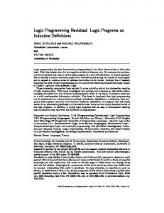
Given a query of reach(a,X), which asks for all states reachable starting from state a, Prolog (using SLD resolution) will search the tree indicated in Figure 1. The atoms to the left of the :- symbols in the tree nodes capture the answers; the list of atoms to the right are waiting to be resolved away. Each path from the root to a leaf is a possible SLD derivation, or in the procedural interpretation of Prolog programs are computation paths through the nondeterministic Prolog program. Notice that the correct answers are obtained, in the three leaves. However, the

reach(a,X) :- reach(a,X) reach(a,X) :- trans(a,X)

reach(a,X) :- trans(a,Intb),reach(Intb,X)

reach(a,b) :-

reach(a,X) :- reach(b,X) reach(a,X) :- trans(b,X) reach(a,c) :-

reach(a,X) :- trans(b,Intc),reach(Intc,X) reach(a,X) :- reach(c,X)

reach(a,X) :- trans(c,X)

reach(a,.X) :- trans(c,Intd),reach(Intd,X)

reach(a,b) :-

reach(a,X) :- reach(b,X)

o

o o o

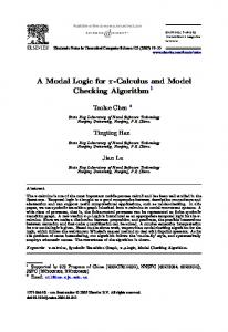
Fig. 1. In nite SLD tree for reach(a,X) point of more interest is that this is an in nite tree, branching in nitely to the lower right. Notice that the lower right node is identical to an ancestor four nodes above it. So the pattern will repeat in nitely, and the computation will never come back to say it has found all answers. A query such as reach(c,a) would go into an in nite loop, never returning to say that a is not reachable from c. Now let us look at the same example executed using SLG resolution in XSB. The program is the same, but we add a directive :- table reach/2. to indicate that all subgoals of reach should be tabled. In this case during execution, an invocation of a reach subgoal creates a new subtree with that subgoal at its root if there is no such tree already. If there is such a tree, then the answers from that tree are used, and no new (duplicate) tree is created. Figure 2 shows the initial partial computation of the same query to the point where the subgoal reach(b,X) is about to be invoked, at the lower right node of that tree. Since reach(a,X) :- reach(a,X) reach(a,X) :- trans(a,X)

reach(a,X) :- trans(a,Intb),reach(Intb,X)

reach(a,b) :-

reach(a,X) :- reach(b,X)

Fig. 2. Initial SLG subtree for reach(a,X) there is no subtree for this subquery, a new one is created and computation

continues with that one yielding another subtree, as shown in Figure 3. Now here reach(b,X) :- reach(b,X) reach(b,X) :- trans(b,X) reach(b,c) :-

reach(b,X) :- trans(b,Intc),reach(Intc,X) reach(b,X) :- reach(c,X)

Fig. 3. Partial SLG subtree for reach(b,X)

reach(c,X) :- reach(c,X) reach(c,X) :- trans(c,X) reach(c,b) :-

reach(c,X) :- trans(c,Intc),reach(Intc,X) reach(c,X) :- reach(b,X)

Fig. 4. Partial SLG subtree for reach(c,X) again a new subgoal, reach(c,X), is invoked, leading to a new subtree, which is shown in Figure 4. Here again we have encountered a subgoal invocation, this time of reach(b,X), and a tree for this subgoal already exists; it is in Figure 3. So no more trees are created (at least at this time.) Now we can use answers in the subtrees to answer the queries in the trees that generated them. For example we can use the answer reach(c,b) in Figure 4 to answer the query of reach(c,X) generated in the lower rightmost node of Figure 3. This results in another answer in Figure 3, reach(b,b). Now the two answers in the tree for reach(b,X) can be returned to the call that is the lower rightmost node of Figure 4, as well as to the lower rightmost node of Figure 2. After all these answers have been returned, no new subgoals are generated, and the computation terminates, having reached a xed point. The nal state of the tree of Figure 2 is shown in Figure 5. The nal forms of the other subtrees reach(a,X) :- reach(a,X) reach(a,X) :- trans(a,X)

reach(a,X) :- trans(a,Intb),reach(Intb,X)

reach(a,b) :-

reach(a,X) :- reach(b,X) reach(a,c) :-

reach(a,b) :-

Fig. 5. The nal SLG subtree for reach(a,X)

are similar. This very simple example shows how tabling in XSB terminates on computations that would be in nite in Prolog. All recursive de nitions over nite sets will terminate in a similar way. Finite-state model checkers are essentially more complicated versions of this simple transitive closure example.

3 Model Checking of Finite-State Systems In this section we present XMC, our XSB-based model checker for CCS and the modal mu-calculus. We rst focus on the alternation-free fragment of the modal mu-calculus, to illustrate the strikingly direct encoding of its semantics as a tabled logic program. The full modal mu-calculus is treated next using a sophisticated semantics for negation developed within the logic-programming community. Finally, we show how the structural operational semantics of CCS, with full value-passing support, can also be naturally captured as a tabled logic program.

3.1 Model Checking the Alternation-Free Modal Mu-Calculus The modal mu-calculus [Koz83] is an expressive temporal logic whose semantics is usually described over sets of states of labeled transition systems. We encode the logic in an equational form, the syntax of which is given by the following grammar:

F ?! Z j tt j ff j F _ F j F ^ F j diam(A, F ) j box(A, F ) D ?! Z += F (least xed point) j Z -= F (greatest xed point) In the above, Z is a set of formula variables (encoded as Prolog atoms) and A is a set of actions; tt and ff are propositional constants; _ and ^ are standard logical connectives; and diam(A, F ) (possibly after action A formula F holds) and box(A, F ) (necessarily after action A formula F holds) are dual modal operators. For example, a basic property, the absence of deadlock, is expressed in this logic by a formula variable deadlock free de ned as: deadlock_free -= box(-, deadlock_free) /\ diam(-, tt)

where the `-' in box and diam formulas stand for any action. The formula states, essentially, that from every reachable state (box(-,deadlock free)) a transition is possible (diam(-,tt)). We assume that the labeled transition system corresponding to the process speci cation is given in terms of a set of facts trans(Src, Act, Dest), where Src, Act, and Dest are the source state, label and target state, respectively, of each transition. The semantics of the modal mu-calculus is speci ed declaratively in XSB by providing a set of rules for each of the operators of the logic, as follows:

models(State_S, tt). models(State_S, (F1 \/ F2)) models(State_S, (F1 \/ F2))

:- models(State_S, F1). :- models(State_S, F2).

models(State_S, (F1 /\ F2))

:- models(State_S, F1), models(State_S, F2).

models(State_S, diam(A, F))

:- trans(State_S, A, State_T), models(State_T, F).

models(State_S, box(A, F))

:- findall(T, trans(State_S, A, T), States_L), map_models(States_L, F).

Consider the rule for diam. It declares that a state State S (of a process) satis es a formula of the form diam(A, F) if State S has an A transition to some state State T and State T satis es F. The semantics of logic programs are based on minimal models, and accordingly XSB directly computes least xed points. Hence, the semantics of the modal mu-calculus's least xed-point operator can be directly encoded as: models(State_S, Z)

:- Z += F, models(State_S, F).

To compute greatest xed points in XSB, we exploit its capability to handle normal logic programs: programs with rules whose right-hand side literals may be negated using XSB's tnot, which performs negation by failure in a tabled environment. In particular, we make use of the duality X:F (X ) = :X::F (:X ), and encode the semantics of greatest xed-point operator as: models(State_S, Z)

:- Z -= F, negate(F, NF), tnot(models(State_S, NF)).

The auxiliary predicate negate(F, NF) is de ned such that NF is a positive formula equivalent to (:F). For alternation-free formulas, the encoding yields dynamically strati ed programs (i.e., a program whose evaluation does not involve traversing loops with negation), and has a two-valued minimal model. In [SSW96] it was shown that the evaluation method underlying XSB correctly computes this class of programs. Tabling ensures that each explored system state is visited only once in the evaluation of a modal mu-calculus formula. Consequently, the XSB program will terminate under XSB's tabling method when there are a nite number of states in the transition system.

3.2 Model Checking the Full Modal Mu-Calculus

Intuitively, the alternation depth of a modal mu-calculus formula [EL86] f is the level of nontrivial nesting of xed points in f with adjacent xed points being of dierent type. When this level is 1, f is said to be \alternation-free". When this level is greater than 1, f is said to \contain alternation." The full modal mu-calculus refers to the class of formulas of all possible alternation depths.

In contrast to the alternation-free fragment of the modal mu-calculus, when a formula contains alternation, the resultant XSB program is not dynamically strati ed, and hence the well-founded model may contain literals with unknown values [vRS91]. For such formulas, we need to evaluate one of the stable models of the resultant program [GL88], and the choice of the stable model itself depends on the structure of alternation in the formula. Such a model can be computed by extending the well-founded model. When the well-founded model has unknown values, XSB constructs a residual program which captures the dependencies between the predicates with unknown values. We compute the values of these remaining literals in the preferred stable model by invoking the stable model generator smodels [NS96] on the residual program. The algorithm used in smodels recursively assigns truth values to literals until all literals have been assigned values, or an assignment is inconsistent with the program rules. When an inconsistency is detected, it backtracks and tries alternate truth assignments for previously encountered literals. By appropriately choosing the order in which literals are assigned values, and the default values, we obtain an algorithm that correctly computes alternating xed points. Initial experiments indicate that XMC computes alternating xed points very eciently using the above strategy, even outperforming existing model checkers crafted to carry out the same kind of computation. Details appear in [LRS98].

3.3 On-the-Fly Construction of Labeled Transition Systems

The above encoding assumes that processes are given as labeled transition systems. For processes speci ed using a process algebra such as CCS [Mil89], we can construct the labeled transition system on the y, using CCS's structural operational semantics. In eect, we can treat trans as a computed (IDB) relation instead of as a static (EDB) relation, without changing the de nition of models. Below, we sketch how the trans relation can be obtained for processes speci ed in XL (a syntactically sugared version of value-passing CCS), the process speci cation language of XMC. The syntax of processes in our value-passing language is described by the following grammar: E ?! PN j in(A) j out(A) j code(C ) j if(C , E , E ) E o E j E '||' E j E # E j E n L j E @ F Def ?! (PN ::= E) In the above, E is a process expression; PN is (parameterized) process name, represented as a Prolog term; C is a computation, (e.g., X is Y+1); Process in(a(t)) inputs a value over port a and uni es it with term t; out(a(t)) outputs term t over port a. Process if(C , E1, E2 ) behaves like E1 if computation C succeeds and otherwise like E2. Operator o is generalized pre xing. The remaining operators are like their CCS counterparts (modulo occasional changes in syntax to avoid clashes with Prolog lexicon). For example, # is nondeterministic choice; '||' is parallel composition; @ is relabeling, where F is a list of

substitutions; and `n' is restriction, where L is a list of port names. Recursion is provided by a set of de ning equations , Def, of the form PN ::= E . The formal semantics of our language is given using structural operational semantics, closely paralleling that of CCS [Mil89]. Due to space limitations, we present here the axioms and inference rules for only a few key constructs. In order to emphasize the highly declarative nature of our encoding, these are presented exactly as they are encoded in the Prolog syntax of XSB. trans(in(A), in(A), nil). trans(out(A), out(A), nil). trans(code(X), _, code) :- call(X). trans(P1 o P2, A, Q) :- trans(P1, A, Q1), (Q1 == code -> trans(P2, A, Q); (Q1 == nil -> Q = P2 ; Q = Q1 o P2))). trans(if(X, P1, P2), A, Q) :- call(X) -> trans(P1, A, Q) ; trans(P2, A, Q). trans( P '||' Q, A, P1 '||' Q ) :- trans(P, A, trans( P '||' Q, A, P '||' Q1) :- trans(Q, A, trans( P '||' Q, tau, P1 '||' Q1) :- trans(P, A, trans(Q, B,

P1). Q1). P1), Q1), comp(A, B).

comp(in(A), out(A)). comp(out(A), in(A)). trans(P, A, Q) :-

P ::= R, trans(R, A, Q).

In the above, A -> B ; C is Prolog syntax for if A then B else C. The trans predicate is of the form trans(P, A, Q) meaning that process P performs an A transition to become process Q. The axiom for input says that in(A) can execute an in(A) transition and then terminate; similarly for the output axiom. The axiom for internal computation forces the evaluation of X and then terminates (without exercising any transition). The rule for generalized pre x states that P1 o P2 behaves like P1 until P1 terminates; at that point it behaves as P2. The conditional process if(X, P1, P2) behaves like P1 if evaluation of X succeeds, and like P2 otherwise. Finally, the rules for parallel composition state that P '||' Q can perform an autonomous A transition if either P or Q can (the rst two rules), and P '||' Q can perform a synchronizing tau transition if P and Q can perform \complementary" actions (the last rule); i.e., actions of the form in(A) and out(A). The nal rule above captures recursion: a process P behaves as the process expression R used in its de nition. To illustrate the syntax and semantics of XL, our value-passing language, consider the following speci cation of a channel chan (with input port get and output port give) implemented as a bounded buer of size N.

chan(N, Buf) ::= code(length(Buf, Len)) o if( (Len == 0) , receive_only(N, Buf) , if( (Len == N) , send_only(N, Buf) , receive_only(N, Buf) # send_only(N, Buf) )). receive_only(N, Buf) ::= in(get(Msg)) o chan(N, [Msg|Buf]). send_only(N,Buf) ::= code(rm_last(Buf,Msg,RBuf)) o out(give(Msg)) o chan(N,RBuf).

In the above de nition rm last(Buf,Msg,RBuf) is a computation, de ned in Prolog, that removes the last message Msg from Buf, resulting in a new (smaller) buer RBuf.

3.4 Implementation and Performance

The implementation of the XMC system consists of the de nition of two predicates models/2 and trans/3; in addition, it contains a compiler to translate input XL representation to one with smaller terms that is more appropriate for ecient runtime processing. Overall the system consists of less than 200 lines of well-documented tabled Prolog code. Preliminary experiments show that the ease of implementation does not penalize the performance of the model checker. In fact, XMC has been shown (see [RRR+97]) to consistently outperform the Concurrency Factory's model checker [CLSS96] and virtually match the performance of SPIN [HP96] on a well-known set of benchmarks. We recently obtained results from XMC on the i-protocol, a sophisticated sliding-window protocol used for le transfers over serial lines, such as telephone lines. The i-protocol is part of the protocol stack of the GNU UUCP package available from the Free Software Foundation, and consists of about 300 lines of C code. Table 1 contains the execution-time and memory-usage requirements for XMC, SPIN, COSPAN [HHK96], and SMV [CMCHG96] applied to the i-protocol to detect a non-trivial livelock error that can occur under certain message-loss conditions. This livelock error was rst detected using the Concurrency Factory. Run-time statistics are given for window sizes W = 1 and W = 2, with the livelock error present (~ xed) and not present ( xed). All results were obtained on an SGI IP25 Challenge machine with 16 MIPS R10000 processors and 3GB of main memory. Each individual execution of a veri cation tool, however, was carried out on a single processor with 1.8GB of available main memory. As can be observed from Table 1, XMC performs exceptionally well on this demanding benchmark. This can be attributed to the power of the underlying Prolog data structuring facility (the i-protocol makes use of non-trivial data structures such as arrays and records), and the fact that data structures in XSB are evaluated lazily.

Version

Tool

Completed? Memory Time (MB) (min:sec) W=1 ~ xed COSPAN Yes 4.9 0:41 SMV Yes 4.0 41:52 SPIN Yes 749 0:10 XMC Yes 18.4 0:03 W=1 xed COSPAN Yes 116 24:21 SMV Yes 5.3 74:43 SPIN Yes 820 1:02 XMC Yes 128 0:46 W=2 ~ xed COSPAN Yes 13 1:45 SMV No 28 >35 hrs SPIN Yes 751 0:12 XMC Yes 68 0:11 W=2 xed COSPAN Yes 906 619:49 SMV No | | SPIN Yes 1789 6:23 XMC Yes 688 3:48 Table 1. i-protocol model-checking results.

4 Beyond Finite-State Model Checking In Section 3 we provided evidence that nite-state model checking can be ef ciently realized using tabled logic programming. We argue here that tabled LP is also a powerful and versatile vehicle for verifying in nite-state systems. In particular, three applications of tabled logic programming to in nite-state model checking are considered. In Section 4.1, we show how an XMC-style model checker can be extended with compositional techniques. Compositional reasoning can be used to establish properties of in nite-state systems that depend only on some nite subpart. Section 4.2 treats parameterized systems. Finally, in Section 4.3, the application of tabled LP to real-time systems is discussed.

4.1 Compositional Model Checking

Consider the XL process A o nil. Clearly it satis es the property diam(A,tt). We can use this fact to establish that (A o nil) # T also satis es diam(A,tt), without consideration of T. This observation forms the basis for compositional model checking , which seeks to solve the model checking problem for complex systems in a modular fashion. Essentially, this is accomplished by examining the syntactic structure of processes rather than the transition relation. (Recall, that the XMC model checker, presented in Section 3, does exactly the latter in its computation of the predicate trans/3.) Besides yielding potentially signi cant eciency gains, the compositional approach is intriguing also when one considers that the T in our example may well have been in nite-state or even unde ned.

Andersen, Stirling and Winskel [ASW94] present an elegant compositional proof system for the veri cation of processes de ned in a synchronous process calculus similar to Milner's SCCS [Mil83] with respect to properties expressed in the modal mu-calculus. A useful feature of their system is the algorithmic nature of the rules. The only nondeterminism in the choice of the next rule to apply arises from the disjunction operator in the logic and the choice of action in the process. Both of these sources of nondeterminism are unavoidable. In this respect, it diers from many systems reported in literature which require a clever choice of intermediate assertions to guide the choice of rules. Andersen et al. in [ASW94] also present an encoding of CCS into their synchronous process calculus and consequently it is possible to use their proof system to verify CCS processes. This encoding, however, has two disadvantages. First, the size of the alphabet increases exponentially with the number of parallel components, and, secondly, the translation of the CCS parallel composition operator is achieved via a complex nesting of synchronous parallel, renaming, and restriction operators. To mitigate the problems with their proof system in the context of CCS, we have adapted it to work directly for CCS processes under the restriction that relabeling operators use only injective functions. Our system retains the algorithmic nature of their system, yet incorporates the CCS parallel composition operator and avoids the costly alphabet blowup. This adaptation is achieved by providing rules at three levels as opposed to two in [ASW94]. The rst level deals with processes that are not in the scope of a parallel composition operator, the second for processes in the scope of a parallel composition operator, and the third for processes appearing in the scope of relabeling and parallel composition operators.

A Level-1 Rule: models(P1 # P2, box(A,F)) :- models(P1, box(A,F)), models(P2, box(A,F)).

A Level-2 Rule: models((P1 # P2) '||'

A Level-3 Rule:

P3, box(A,F)) :models(P1 '||' P3, box(A, F)), models(P2 '||' P3, box(A, F)).

models((B o P1) @ R '||' P2, box(A,F)) :maps(R,B,C), models(C o (P1 @ R) '||' P2, box(A,F)).

Our system is sound for arbitrary processes and complete for nite-state processes. It has been implemented using XSB in the same declarative fashion as our XMC model checker. The compositional system is expected to improve on XMC's space eciency by avoiding the calculation of intermediate states and by reusing subproofs, though worst-case behavior is unchanged. Performance evaluation is ongoing.

Our compositional system can indeed provide proofs for properties of partially de ned processes as illustrated by the following example from [ASW94]. Let p ::= (tau o p) # T and q ::= (tau o q) # T where T is an unspeci ed process. The formula x += box(tau, x) expresses the impossibility of divergence. The following is a proof that p '||' q may possibly diverge. models(p '||' q, x) ?- models(p '||' q, box(tau, x)) ?- models((tau o p) # T) '||' q, box(tau, x)) ?- models((tau o p) '||' q, box(tau, x)) ?- models(p '||' q, x) ?- fail.

4.2 Model Checking Parameterized Systems using Induction We have thus far described how inference rules for a variety of veri cation systems can be encoded and evaluated using XSB. These inference systems specify procedures that are primarily intended for model checking nite-state systems. We now sketch how more powerful deductive schemes oer (albeit incomplete) ways to verify properties of parameterized systems . A parameterized system represents an in nite family of nite-state systems; examples include an n-bit shift register and a token ring containing an arbitrary number of processes. An in nite family of shift registers can be speci ed in XL as follows: reg(0) :== bit reg(s(N)) :== (bit @ [get/temp] || reg(N) @ [give/temp]) \ {temp} bit :== in(get) o out(give) o bit

In the above speci cation, natural numbers are represented using successor notation (0, s(0), s(s(0)), : : :) and reg(n) de nes a shift register with n + 1 bits. Now consider what happens when the query models(reg(M), ), for some nontrivial property  and M unbound (thereby representing an arbitrary instance of the family), is submitted to an XMC-style model checker. Tabled evaluation of this query will attempt to enumerate all values of M such that reg(M) models the formula . Assuming there are an in nite number of values of M for which this is the case, the query will not terminate. Hence, instead of attempting to enumerate the set of parameters for which the query is true, we need a mechanism to derive answers that compactly describe this set. For this purpose, we exploit XSB's capability to derive conditional answers: answers whose truth has not yet been (or cannot be) independently established. This mechanism is used already in XSB for handling programs with non-strati ed negation under well-founded semantics. For instance, for the program fragment p :- q. q :- tnot r. r :- tnot q. XSB generates three answers: one for p that is conditional on the truth of q, and one each for q and r, both conditional on the falsity of the other. Now, if r can be proven false independently, conditional

answers for q and p can be simpli ed : both can be marked as unconditionally true. Our approach to model checking parameterized systems is to implement a scheme to uncover the inductive structure of a veri cation proof based on the above mechanism for marking and simplifying conditional answers. Consider, again, the query models(reg(M), ). When resolving this query, we will encounter two cases, corresponding to the de nition of the reg family: (i) M = 0, and (ii) M = s(N), corresponding to the base case and the recursive case, respectively. For the base case, the model checking problem is nite-state and the query models(reg(0), ) can be completely evaluated by tabled resolution. For the recursive case, we will eventually encounter a subgoal of the form models(reg(N), 0 ), where 0 is some subformula of . For simplicity of exposition, consider the case in which  = 0. Under tabled resolution, since this subgoal is a variant of one seen before, we will begin resolving answers to models(reg(N), ) from the table of models(reg(M), ), and eventually add new answers to models(reg(M), ). This naive strategy leads to an in nite computation. However, instead of generating (enumerating) answers for models(reg(N), ) for adding answers to models(reg(M), ), we can generate one conditional answer, of the form: models(reg(M),

)

:- M = s(N), models(reg(N),

).

which captures the dependency between the two sets of answers. In eect, we have evaluated away the nite parts of the proof, \skipping over" the in nite parts while retaining their structure. For instance, in the above example, we skipped over models(reg(N), ) (i.e., did not attempt to establish its truth independently), and retained the structure of the in nite part by marking the truth of models(reg(s(M)), ) as conditional on the truth of models(reg(N), ). Using this mechanism, we are left with a residual program, a set of conditional answers that re ects the structure of the inductive proof. The residual program, in fact, computes exactly the set of instances of the family for which the property holds, and hence compactly represents a potentially in nite set. Resolution as sketched above, by replacing instances of heads (left-hand sides) of rules by the corresponding bodies (right-hand sides) unfolds the recursive structure of the speci cation. In order to make the structure of induction explicit, it is often necessary to perform folding steps, where instances of rule bodies are replaced by the corresponding heads. In [RRRS98] we describe how tabled resolution's ability to compute conditional answers, and folding mechanisms can be combined to reveal the structure of induction. It should be noted that although we have a representation for the (in nite) set of instances for which the property holds, the proof is not yet complete; we still need to show that the set of instances we have computed covers the entire family. What we have done is to simply evaluate away the nite parts, leaving behind the core induction problem, which can then be possibly solved using theorem provers. In many cases, however, the core induction problem is simple enough that the proof can be completed by heuristic methods that attempt to nd a counter example, i.e., an instance of the family that is not generated by the

residual program. For example, we have successfully used this counter-example technique to verify certain liveness properties of token rings and chains (shift registers), and soundness properties of carry look-ahead adders.

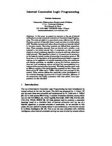
4.3 Model Checking Real-Time Systems Another kind of in nite-state system we are interested in is real-time systems . Most embedded systems such as avionics boxes and medical devices are required to satisfy certain timing constraints, and real-time system speci cations allow a system designer to explicitly capture these constraints. Real-time systems are often speci ed as timed automata [AD94]. A timed automaton consists of a set of locations (analogous to states in a nite automaton), and a set of edges between locations denoting transitions. Locations as well as transitions may be decorated with constraints on clocks . An example of a timed automaton appears in Figure 6. A state of a timed automaton comprises a location and an assignment of values to clock variables. Clearly, since clocks range over in nite domains, timed automata are in nite-state automata. Real-time extensions to temporal logics, such as timed extensions of the modal mu-calculus [ACD93,HNSY94,SS95], are used to specify the properties of interest. Traditional model-checking algorithms do not directly work in the case of real-time systems since the underlying state-space is in nite. The key then is to consider only nitely many regions of the state space. In [AD94] it is shown that when the constraints on clocks are restricted to those of the form X < Y + c where X and Y are clock variables and c is a constant, the state space of a timed automaton can be partitioned into nitely many stable regions|sets of indistinguishable elements of the state space. For example, in the automaton of Figure 6, states hL0 ; t = 3i and hL0 ; t = 4i are indistinguishable. States hL0 ; t = 4i and hL0 ; t = 6i, however, can be distinguished, since only from the latter can we make a transition to hL1 ; t = 6i, where an a-transition is enabled.

t>1

t>2

b

a

L0

a

L1

d

c

reset t

t>5

L2 t