int. j. remote sensing, 1998 , vol. 19, no. 18 , 3499± 3514
Logistic regression modelling of multitemporal Thematic M apper data for burned area mapping N. KOUTSIAS³ and M. KARTERIS Department of Forestry and Natural Environment, Laboratory of Forest Management and Remote Sensing, Box 248 , Aristotelian University, 540 06 Thessaloniki, Greece (Received 2 7 May
1997;
in ® nal form 2 4 December 1 9 9 7 )
This study focused on the development of a logistic regression model for burned area mapping using two Landsat- 5 Thematic Mapper (TM) images. Logistic regression models were structured using the spectral channels of the two images as explanatory variables. The overall accuracy of the results and other statistical indications denote that logistic regression modelling can be used successfully for burned area mapping. The model that consisted of the spectral channels TM4 , TM7 and TM1 and had an overall accuracy of 97 .62 %, proved to be the most suitable. Moreover, the study concluded that the spectral channel TM4 was the most sensitive to alterations of the spectral response of the burned category pixels, followed by TM7 . Abstract.
1.
Introduction
A well structured decision-making system for the management of forest ® res needs a complete and accurate geographical database of burned areas. Appropriate statistics of ® re occurrence on a permanent basis will help ® re managers to better understand the ® re problem, including the reasons for ® re ignition and spreading. On the other hand, the collection of those statistics should rely on cost-e ective, quick and accurate methods. Satellite remote sensing seems to be a promising approach for collecting information on ® re occurrence, since it provides the necessary means of gathering information of the Earth’s surface in a less expensive and timely fashion. Among the multivariate techniques used to predict a binary dependent variable from a set of independent variables, multiple regression and discriminant analysis are widely applied. However, both techniques show limited value when the dependent variables takes only two values, that is, whether an event occurs or not. Under these circumstances, the assumption needed to test the hypothesis in regression analysis are violated (Norusis 1990 ). In such cases, another multivariate technique, that of logistic regression which is used for estimating the probability of an event occurring, is applied. So far, various logistic regression models have been structured and evaluated in a wide range of applications. This approach proved useful in examining the relationship between a set of independent variables and a dependent variable which takes only two dichotomous values (Pereira and Itami 1991 , Boxall and McFarlane 1995 , Bian and West 1997 , Narumalani et al. 1997 , van Deventer et a l. 1997 ). Especially in the ® elds of remote sensing, Geographic Information System ³ E-mail:
[email protected] 0 143 ± 1161 / 98 $12 .0 0
Ñ
1998 Taylor & Francis Ltd
3500
N. Koutsias and M. Karteris
(GIS) and wild® res, logistic regression modelling has been applied to examine the relationship between National Fire Danger Rating System (NFDRS) indices and ® re occurrence (Loftsgaarden and Andrews 1992 ), to predict the daily people-caused ® re occurrence (Martell et a l. 1987 ), to predict post-® re mortality in certain species (Ryan and Reinhardt 1988 ), and to model the distribution of ® re occurrence probability for estimating ® re danger (Chou et a l. 1990 , Chou 1992 ). In the case of burned area mapping, logistic regression models can be structured for estimating the probability based on whether or not a pixel belongs to a burned area and consequently can be classi® ed as burned or unburned. The nature of the problem allows the structure and evaluation of such regression models, since the dependent variable in this case can be treated as a variable which takes only two dichotomous values. The problem now is how to classify the pixels of a satellite image having a criterion whether or not a pixel belongs to a burned area. The main advantage of this approach is the simpli® cation of the problem. Consequently, in order to be able to structure a logistic regression model, it is necessary to determine certain training areas on a satellite image for which it is known that they belong either to burned or to unburned areas. In the case of burned category pixels, the dependent variable is coded to the value 1 , while for the unburned pixels the dependent variable is coded to the value 0 . The set of the independent variables consists of the spectral channels of the pre® re and post-® re satellite image and consequently the values of each independent variable are actually the radiometric values of the pixels in each spectral channel. 2.
M aterials and methods 2 .1 . Stu dy a rea an d ex p lan ato ry va riab les In September 1992 a large ® re occurred in the northern part of Attica in Greece (® gure 1 ) over Lake Marathon and burned about 5500 h. This was the study area
for the application of the logistic regression model in burned area mapping. For this purpose, two successive satellite images of Landsat- 5 Thematic Mapper (TM) taken on 26 August (before the ® re) and 11 September ( just after the ® re) were acquired. A subset including a broad area around the ® re extent was extracted from the two original satellite images (® gures 2 and 3 ) and constituted the basic source of information. To make feasible the incorporation and further coprocessing of the two satellite images, geometric registration, based on the manual identi® cation of 36 control points over both images with a maximum accepted RMS error of 0 .5 , was applied to the data set. Afterwards, one of the two images was transformed to ® t geometrically with the other, using a ® rst-order polynomial and nearest neighbour resampling method (Fonseca and Manjunath 1996 ). An evaluation of the geometric registration technique applied in this data set showed a satisfactory overall success, although in some cases small deviations appeared due to radiometric deviations between the two images and temporal changes in land cover/ use (clouds, etc.). The evaluation of the geometric registration was performed based on the di erence of Normalized Di erence Vegetation Index (NDVI) values of the pre- and post-® re satellite images. The last step of the image pre-processing procedure was the radiometric restoration and image-to-image matching. Simple statistics such as mean, minimum, maximum, etc., were extracted from both images, since the radiometric restoration in this study concerned only the haze removal based on the minimum values in each
L ogistic regression modelling for burned area mapping
3501
Figure 1 . Geographical location of the study area.
spectral channel (Sabins 1986 ). The minimum value of each spectral channel was subtracted from each pixel brightness in that channel. Having completed all the pre-processing procedures for making the two images compatible, a common window of 600 rows and 663 columns was extracted. The ® nal window included 12 spectral channels (except TM6 ) that were treated in further analysis as the explanatory variables. 2 .2 . L o gistic reg ression mo d el fo r b u rne d a rea ma p pin g
In the case of a multivariate data set, such as in remotely sensed data taken from LANDSAT TM, the probability of an event occurring is given by the following general regression model (Mendenhall and Sincich 1996 ): E (y)=
exp (b 0 + b 1 X 1 + b 2 X 2 + . . . + b k X k ) 1 + exp (b 0 + b 1 X 1 + b 2 X 2 + .. . + b k X k )
where y=
G
1
0
(1 )
if category A occurs if category B occurs
E (y)= P (Category A occurs) = p , X 1 , X 2 , ..., X k are quantitative or qualitative independent variables and b 0 , b 1 , ..., b k are the estimated coe cients. In addition to linear regression in which the coe cients of the model are estimated using the method of
3502
N. Koutsias and M. Karteris
Figure 2 . The Landsat- 5 TM satellite image acquired on 26 August 1992 before the ® re.
least squares, in logistic regression the coe cients of the model are estimated using the maximum likelihood method. In other words, the selected coe cients are those which make the observed results most likely (Norusis 1990 ). For burned area mapping the above general regression model remains the same, while the event is de® ned whether or not the pixel belongs to the burned area. Thus, the logistic expression denotes the probability based on whether a pixel belongs to a burned area. In this case, the set of the independent variables consists of the spectral channels of two Landsat images taken before and after the ® re. 2 .3 . E stab lishm ent of th e d a ta set
Having completed all the necessary actions to establish the database concerning the broad area around the ® re perimeter, the next and most crucial step was to obtain a satisfactory sample size from both images. In other words, it was necessary to determine certain areas and code them either with the value 1 when the sample corresponded to burned area or 0 when the sample corresponded to unburned areas. The success of the logistic regression modelling was dependent upon the accurate location of these sampling areas. A certain set of prerequisites should be ful® lled to ensure the validity of the
L ogistic regression modelling for burned area mapping
3503
Figure 3 . The Landsat- 5 TM satellite image acquired on 11 September 1992 , just after the ® re. The spectral channels TM7 , TM4 and TM1 displayed in red, green and blue colour plane enhance the discrimination of burned areas. The burned areas appear as dark red, while vegetative areas are green, the sea dark blue and the bare land, clouds and urban areas are white.
development, evaluation and application of the logistic regression model, as well as the interpretation of the results. These prerequisites were the following: 1 . The sampling areas corresponding to the burned and unburned areas should be accurately determined over both satellite images. The analysis showed that the colour composite consisting of TM7 , TM4 and one of TM1 , TM2 or TM3 displayed in red, green and blue colour plane, respectively, allowed better visual location of these sampling areas. This speci® c false colour composite enhanced the visual discrimination between burned land and other land cover/ use categories. The burned areas appeared as dark red, while vegetation areas appeared as green, the sea as dark blue and the bare land, clouds and urban areas as white. 2 . The sample size for the burned and the unburned areas should be about the same. The analysis showed that if the sample size di ers greatly between burned and
3504
N. Koutsias and M. Karteris
unburned areas, the results would be biased. Moreover, for both cases, a satisfactory absolute sample size should be obtained. 3 . The sampled areas should represent all the variability occurring on the satellite images, within and outside the burned area. The analysis showed that the exclusion of certain characteristics, such as clouds or shadows, creates undesirable results. In other words, the sampling areas should be determined based on the same criteria followed in the case of a detailed supervized classi® cation. Based on the above prerequisites, 11 small windows each consisting of 36 rows and 31 columns ( 1116 pixels in each window), were assessed on both images. Six of the 11 windows represented the whole variability outside the burned area and were coded with the value of 0 , while the rest represented the whole variability inside the burned area and were coded with the value of 1 . Thus, the sample size of the burned area consisted of 5580 pixels and the unburned area 6696 . The ® nal step in preparing the data set was to extract the radiometric values included in the identi® ed windows and store them in an ASCII format ® le. This data set consisted of 12 276 observations, 12 explanatory independent variables and one response-dependent variable. 3.
Results and discussion 3 .1 . E valuatio n of th e da ta set
Before continuing with logistic regression analysis, a simple statistical evaluation of the 11 sampling areas was performed to acquire a ® rst indication about the level of discrimination between burned and unburned samples. The statistical analysis was directed to show the distribution of each spectral channel to the overall discrimination and how well each channel performs in discriminating and mapping burned areas. Some of the simple statistics and the histogram data plots which were extracted from both satellite images are depicted in ® gures 4 and 5 . Regarding the discrimination between burned and unburned samples, it is apparent (® gure 5 ) that among spectral channels the re¯ ective infrared channel (TM4 ) o ered the highest discrimination. The spectral response of the burned category pixels has been decreased compared to the pre-® re condition. The average radiometric value of the sampling area before the ® re was 43 .12 , while it had been reduced to 17 .56 after the ® re. The reduction is due to the removal of the vegetation layer which re¯ ects large amounts of the incident radiation in this spectral channel. The second channel that performs well in the discrimination of burned and unburned areas is the mid-infrared (TM7 ). The spectral response of the burned category pixels, in addition to spectral channel TM4 , increased considerably compared with the pre® re condition. The average radiometric value before the ® re was 23 .11 while the corresponding value after the ® re increased to 40 .20 . The spectral response of burned pixels in the visible part of the electromagnetic spectrum slightly increased compared with the pre-® re situation, although such an increase was not signi® cant. Finally, in spectral channel TM5 the spectral response of burned pixels was not altered between the pre- and post-® re satellite images, since the mean radiometric values were 52 .65 and 51 .37 , respectively. Consequently, this spectral channel does not o er any di erentiation between burned and unburned areas. Regarding the histogram data plots of the sampling area corresponding to the unburned case, it was evident that the spectral response of the sampling pixels in the pre- and post-® re image was similar. This means that the haze removal applied
L ogistic regression modelling for burned area mapping
3505
( a)
( b)
Figure 4 . Histogram data plots and simple statistics of a random sampling of the burned area, on the pre-® re satellite image (a ) and on the post-® re satellite image (b ).
to both images eliminated the atmospheric in¯ uence and produced a new data set in which unchanged areas had a similar spectral response. 3 .2 . Structure a nd ev alua tion o f log istic reg ression mo d els
After the preparation of the sampled data set and having acquired a ® rst indication about the potential di erentiation between burned and unburned areas o ered
3506
N. Koutsias and M. Karteris
Figure 5 . Histogram data plots of a random sampling of the burned area. The histogram data appearing in black corresponds to the pre-® re image data, while the grey corresponds to the post-® re image data. It is evident that among spectral channels, TM4 and TM7 o er the highest discrimination between burned and unburned areas.
by each spectral channel, the next step was to create and evaluate the logistic regression models. Apart from the structure and evaluation of the ® nal model, speci® c objectives of the regression analysis were to quantify the performance of each spectral channel in the overall discrimination of burned areas and compare the results with those obtained with the histogram data plot comparisons. In logistic regression, as well as in multiple regression, it is di cult to estimate the contribution of individual variables
L ogistic regression modelling for burned area mapping
3507
in predicting the response variable, since the contribution of each variable depends on other variables presented in the model. This problem is especially noticeable when the independent variables are highly correlated (Norusis 1990 ) as in the case of TM data. To overcome these limitations regarding the interpretation of the coe cients of the model, six di erent models consisting of one spectral channel from both satellite images were structured and evaluated. Before presenting the results acquired from the above six logistic models, a few points concerning the criteria used to evaluate how well a logistic regression model predicts the response variable should be clari® ed. The ® rst indication is taken from the classi® cation table (table 1 ) based on the comparisons between the predicted and the observed outcomes. Apart from the overall weighted percentage of correct classi® ed observations, the sub-accuracies of the burned and unburned cases should be taken into consideration. In general, good models are those which result in high overall per cent accuracy with the prerequisite that both of the two groups contribute the same to the ® nal overall accuracy. Table 1 summarizes the results taken from the structure of a logistic regression model. Although table 1 provides the overall weighted percentage of correct classi® ed observations, however it does not reveal the distribution of the estimated probabilities of the two groups. This limitation was overcome by displaying the histogram plot of the estimated probabilities (® gure 6 ). In the case that the model successfully distinguishes the two groups of the dependent variable, then these groups should be clustered at their respective ends of the plot. According to these two criteria, the performance of the logistic model is determined upon how well the model classi® es the observations. In addition, a di erent approach to assess the goodness of ® t of the model is to examine certain statistics, such as the Õ 2 times the log of the likelihood (Õ 2 LL) and the goodness of ® t statistic. Good models are considered to be those that result in small values of Õ 2 LL and the goodness of ® t statistic. Table 1 . Classi® cation table for observed and predicted results of a logistic regression model. Observed
Unburned ( 0 ) Burned ( 1 )
Predicted
Percentage correct
Unburned ( 0 )
Burned ( 1 )
4490 3212
2206 2368
67 .05 % 42 .44 %
Overall:
5 5 .8 7 %
Figure 6 . Observed groups and predicted probabilities using a logistic regression model. The initial values of the model ( 0 ± 1 ) have been rescaled to 0 ± 100 .
3508
N. Koutsias and M. Karteris
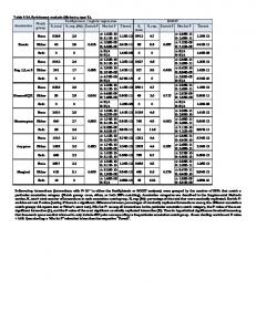
Table 2 summarizes the results acquired from the construction of the models, which include only one spectral channel from pre- and post-® re satellite image. The overall percentage of correct classi® ed observations in each logistic model indicates the performance of each model and consequently determines the contribution of each spectral channel to the discrimination and mapping of burned areas. The conclusion that arise from table 2 are exactly the same as those extracted from the statistical analysis and histogram data plot comparisons. Again, the spectral channel TM4 , before and after the ® re, provided the highest accuracy ( 89 .89 %), which denotes that the spectral information content in this channel contributes signi® cantly in burned area mapping. The spectral channel TM4 proved to be the most sensitive regarding alterations in spectral response of the pixels of the burned areas. The spectral channel with the second highest contribution to burned area discrimination was TM7 , for which the overall percentage of correctly classi® ed observations was 82 .84 %. Regarding the visible channels, TM1 seems to be the most valuable among the three, since its overall accuracy was 55 .87 % compared to TM2 and TM3 where it was 43 .68 % and 33 .02 %, respectively. Finally, for the spectral channel TM5 the overall accuracy was 49 .67 % (table 2 ). However, this value did not re¯ ect the real performance of the model, since it was estimated from the weighted mean of both sub-accuracies, which were 86 .87 % for unburned and only 5 .04 % for burned observations. Actually, this model predicted the unburned observations well ( 86 .87 %), but did not predict the burned observations ( 5 .04 %). This case denotes that the evaluation of the performance of the model should rely upon di erent criteria. Conclusions extracted from the interpretation of the classi® cation tables and the histogram data plot comparisons, were also veri® ed, by comparing the statistics of Õ 2 times the log likelihood and the goodness of ® t statistic. 3 .3 . Deve lop men t a nd a p plica tion o f th e log istic reg ression mo d els
Having determined the performance of each spectral channel to the overall discrimination of burned and unburned areas, three di erent logistic regression models were constructed and tested. The ® rst included only the two channels that performed best, that is TM4 and TM7 , before and after the ® re. Thus, four explanatory variables (TM4 , TM7 of both satellite images) set up the data set. Table 3 summarizes the results of the model which presented an overall accuracy of 97 .69 %, while the Õ 2 LL was 1788 .4 and the goodness of ® t statistic 27075 .09 . The second model included the three spectral channels that performed best, that is TM4 , TM7 and TM1 . The overall accuracy in this case was 97 .79 % while the Õ 2 LL was 1702 .2 and the goodness of ® t 18370 .58 . The results are summarized in table 4 . Finally, the third logistic regression model included all spectral channels, before and after the ® re. In this case, the model gave the maximum performance in predicting the response variable. Its overall accuracy was 97 .96 %, while the Õ 2 LL was 1547 and the goodness of ® t 6906 .5 . Table 5 summarizes the results of the third model. In comparison, these three models are similar in performance, since their overall accuracy does not signi® cantly di er. However, other statistics such as the goodness of ® t and Õ 2 LL, as well as the graphs which represent the distribution of the estimated probabilities for the prediction of the response variable, which better justify the performance of each model, should be taken into consideration in the ® nal
Unburned ( 0 ) Burned ( 1 )
Observed
5 5 .8 7 %
Overall:
3594 5121
Unburned ( 0 )
3 3 .0 2 %
Overall:
5817 5299
Unburned ( 0 )
Overall:
879 281
Burned ( 1 )
4 9 .6 7 %
86 .87 % 5 .04 %
Percentage correct
53 .67 % 8 .23 %
3102 459
Burned ( 1 )
Percentage correct
67 .05 % 42 .44 %
Percentage correct
2206 2368
Burned ( 1 )
Model 5 : TM5 before and after the ® re event Predicted
Unburned ( 0 ) Burned ( 1 )
Observed
4490 3212
Unburned ( 0 )
Model 3 : TM3 before and after the ® re event Predicted
Unburned ( 0 ) Burned ( 1 )
Observed
Model 1 : TM1 before and after the ® re event Predicted
Unburned ( 0 ) Burned ( 1 )
Observed
Overall:
2735 1401
Burned ( 1 )
5876 421
Unburned ( 0 )
Overall:
820 5159
Burned ( 1 )
5895 1306
Unburned ( 0 )
Overall:
801 4274
Burned ( 1 )
Model 6 : TM6 before and after the ® re event Predicted
Unburned ( 0 ) Burned ( 1 )
Observed
3961 4179
Unburned ( 0 )
Model 4 : TM4 before and after the ® re event Predicted
Unburned ( 0 ) Burned ( 1 )
Observed
Model 2 : TM2 before and after the ® re event Predicted
8 2 .8 4 %
88 .04 % 76 .59 %
Percentage correct
8 9 .8 9 %
87 .75 % 92 .46 %
Percentage correct
4 3 .6 8 %
59 .15 % 25 .11 %
Percentage correct
Table 2 . Classi® cation tables for the logistic regression models which include only one channel from the pre-® re and post-® re satellite images.
L ogistic regression modelling for burned area mapping 3509
N. Koutsias and M. Karteris
3510
Table 3 . Classi® cation table and statistical performance of the ® rst model (variables: TM4 and TM7 before and after ® re). Observed
Unburned ( 0 ) Burned ( 1 )
Predicted
Percentage correct
Unburned ( 0 )
Burned ( 1 )
6609 196
87 5384
98 .70 % 96 .69 %
Overall:
9 7 .6 9 %
log likelihood = 1788 .42 Goodness of ® t = 27075 .09 2
Õ
Table 4 . Classi® cation table and statistical performance of the second model (variables: TM4 , TM7 and TM1 ). Observed
Unburned ( 0 ) Burned ( 1 )
Predicted
Percentage correct
Unburned ( 0 )
Burned ( 1 )
6614 189
82 5391
98 .78 % 96 .61 %
Overall:
9 7 .7 9 %
log likelihood = 1702 .20 Goodness of ® t = 18370 .58 2
Õ
Table 5 . Classi® cation table and statistical performance of the third model (variables: all spectral bands). Observed
Unburned ( 0 ) Burned ( 1 )
Predicted
Percentage correct
Unburned ( 0 )
Burned ( 1 )
6620 175
76 5405
98 .86 % 96 .86 %
Overall:
9 7 .9 6 %
Õ
log likelihood = 1547 .81 Goodness of ® t = 6906 .53
2
conclusions. In this study those graphs have been produced after the application of each model for the whole image. The estimated coe cients of each logistic model as well as other statistics which re¯ ect the contribution of each variable to the overall performance, are presented in table 6 . In this table the column heading B represents the estimated coe cients of each explanatory variable. The standard errors of the logistic regression coe cients are shown in column labelled SE, while the Wald statistic and its signi® cance level is shown in column labelled Wald and p , respectively. The partial correlation between the dependent variable and each of the independent variables is given in the column labelled R , which indicates the behaviour of the likelihood of the event occurring in relation to the behaviour of the independent variable. These statistics give an indica-
L ogistic regression modelling for burned area mapping
3511
Table 6 . Parameter estimates for the three logistic regression models. Variables
B
SE
Wald
p
R
First model: T M 4 and T M 7 before and after the ® re
TM4 Ð Post TM7 Ð Post TM4 Ð Pre TM7 Ð Pre Constant
0 .4413 0 .3958 0 .2100 0 .1438 4 .7512
Õ
Õ
Õ
0 .0137 0 .0121 0 .0085 0 .0084 0 .1779
1031 .58 1064 .63 603 .69 293 .26 713 .40
0 .0000 0 .0000 0 .0000 0 .0000 0 .0000 Õ
Õ
Second model: T M 4 , T M 7 and T M 1 before and after the ® re
TM1 Ð Post TM4 Ð Post TM7 Ð Post TM1 Ð Pre TM4 Ð Pre TM7 Ð Pre Constant
0 .0857 0 .3990 0 .4531 0 .0164 0 .1575 0 .1548 2 .7709
Õ
Õ
Õ
Õ
Õ
0 .0111 0 .0140 0 .0149 0 .0108 0 .0108 0 .0118 0 .3100
59 .77 811 .24 922 .53 2 .29 213 .24 172 .15 79 .87
0 .0000 0 .0000 0 .0000 0 .1294 0 .0000 0 .0000 0 .0000
T hird model: all spectral bands before and after the ® re
TM1 Ð Post TM2 Ð Post TM3 Ð Post TM4 Ð Post TM5 Ð Post TM7 Ð Post TM1 Ð Pre TM2 Ð Pre TM3 Ð Pre TM4 Ð Pre TM5 Ð Pre TM7 Ð Pre Constant
Õ
Õ
Õ
Õ
Õ
Õ
0 .0827 0 .1615 0 .1420 0 .3661 0 .1107 0 .5759 0 .0075 0 .2683 0 .2081 0 .1245 0 .1193 0 .3166 3 .4317
0 .0235 0 .0596 0 .0412 0 .0232 0 .0138 0 .0268 0 .0257 0 .0650 0 .0420 0 .0146 0 .0146 0 .0272 0 .4637
12 .37 7 .35 11 .90 247 .95 64 .58 462 .82 0 .08 17 .05 24 .50 72 .37 66 .61 135 .72 54 .78
0 .0004 0 .0067 0 .0006 0 .0000 0 .0000 0 .0000 0 .7706 0 .0000 0 .0000 0 .0000 0 .0000 0 .0000 0 .0000
0 .2467 0 .2506 0 .1886 0 .1312
0 .9179 0 .6710 1 .5733 0 .9837 1 .1705 0 .8566
0 .9206 0 .8509 1 .1526 0 .6935 0 .8952 1 .7788 1 .0075 1 .3077 0 .8121 1 .1326 1 .1267 0 .7286
B, estimated coe cients of each explanatory variable.
tion of the signi® cance of each variable, although to estimate the actual contribution of each variable, it would be necessary to build a model with and without that variable and test the results. As has been mentioned, the behaviour of each variable depends on the other variables in the model, especially when the independent variables are highly correlated. The ® nal evaluation of the three speci® ed logistic models, as well as the selection of one of them relied on the following three criteria: 1 . How distinct was the distribution of the estimated probabilities of the response
variable; highly discrete groups indicate good performance. 2 . How many channels are included in the model which is related to the total cost; less variables indicate time and money savings. 3 . The ® nal accuracy of the classi® cation results; high accuracy indicate good performance. Based on the above criteria there was no signi® cant di erence among the three models, although a detailed examination of the frequency value led to the conclusion that the second model (TM4 , TM7 , TM1 ) gave a slightly better performance. Moreover, the ® rst and second model satis® ed the second criterion since they
N. Koutsias and M. Karteris
3512
Table 7 . Accuracy assessment of the results of the three logistic regression models for burned area mapping. Category information Observed Unburned ( 0 ) Burned ( 1 )
Estimated Unburned ( 0 ) Burned ( 1 ) Unburned ( 0 ) Burned ( 1 )
Overall
First model Cell count 332 615 323 259 9356 65 185 4371 60 814
% accuracy 97 .19 2 .81 6 .71 93 .29 96 .54
Second model Cell count 332 615 323 166 9449 65 185 3963 61 222
% accuracy 97 .16 2 .84 6 .08 93 .92 97 .62
Third model Cell count 332 615 323 709 9906 65 185 4085 61 100
% accuracy 97 .02 2 .98 6 .27 93 .73 96 .73
included 4 and 6 variables, respectively, in contrast to the third model which included 12 . Finally, based on the visual evalution of the spatial distribution of the classi® cation results, all three models showed a similar behaviour, although a detailed examination led to the conclusion that model 2 (TM4 , TM7 , TM1 ) performed slightly better. Evaluating the classi® cation results of the logistic regression model, the overall success of the proposed methodology was evident, although in some cases small deviations appeared due to geometric misregistration in local level, radiometric deviations between the two images, and the temporal changes in land cover/ use. All these deviations can be easily eliminated by applying `clumping’ and `sieving’ techniques supported in ERDAS 7 .5 version. 4.
Accuracy assessment
After the application of the three di erent logistic regression models and having acquired a ® rst indication about how successful the analysis was based on the statistical indications, the last step was the evaluation of the classi® cation results and the accuracy assessment. Since there were no available detailed maps or aerial photographs depicting the actual boundaries of the burned area, the accuracy assessment relied on information derived from manual interpretation of the satellite image taken after the ® re event. The colour composite of TM7 , TM4 and TM1 , displayed in red, green and blue colour planes respectively was used to extract the exact boundaries of the burned area. Although the methodology applied does not ensure a perfect means to achieve a reference map of the burned area, it can be applied to acquire one more indication about the success of the logistic regression modelling approach. Table 7 provides the results of the accuracy assessment of the three logistic regression models. From this table, it is obvious that all three logistic regression models performed well for burned area mapping without having signi® cant di erences. However, the second model has been chosen, since it produces slightly better results. 5.
Conclusions
The primary objective of this study was to examine whether logistic regression modelling of Landsat- 5 TM data acquired before and after a ® re could be applied
L ogistic regression modelling for burned area mapping
3513
in burned area mapping. The statistical indications, which have arisen from the structure and application of the logistic regression models and the estimated accuracies, show that the proposed methodology can be applied in burned area mapping with promising results. The estimated accuracies of above 90 %, based on data derived by manual interpretation of the post-® re satellite image for the three structured logistic models, are considered to be very high. The logistic model consisting of the spectral channels TM4 , TM7 and TM1 presented the maximum overall accuracy ( 97 .62 %) and proved to be the most suitable for burned area mapping. Apart from the structure and application of the ® nal logistic model, another objective of this study was the estimation of the performance of each spectral channel in the overall discrimination of burned areas. The spectral channel TM4 proved to be the most sensitive regarding alterations in spectral response of the burned pixels and consequently performed the best. The spectral channel with the second highest contribution to burned area discrimination was TM7 . Regarding the visible part of the electromagnetic spectrum, the spectral channel TM1 seemed to be the most valuable among the three, while the spectral channel TM5 did not o er any distinctiveness. In conclusion, logistic regression modelling applied to multitemporal satellite data proved to be a suitable statistic tool in predicting a dependent variable that takes only two values and consequently can be used in a classi® cation process when the classi® cation problem can be de® ned in a dichotomous way. However, further research, which will include comparisons with other techniques and evaluation of the proposed methodology in other cases, is needed in order to develop an operational and accurate method for burned area mapping using satellite data. Acknowledgments
This research was (in part) supported by the EC Environment and Climate Research Programme (contact ENV4 -CT95 -0256 Climatology and Natural Hazards). References B ian, L ., and W est, E ., 1997 , GIS modeling of elk calving habitat in a prairie environment with statistics. P hoto grammetric E ngine ering and R emo te Sensing, 6 3 , 161 ± 167 . B oxall, P . C ., and M c F arlane, B . L ., 1995 , Analysis of discrete, dependent variables in
human dimensions research: participation in residential wildlife appreciation: W ild life Society B ulletin , 2 3 , 283 ± 289 . C hou, Y . H ., 1992 , Management of wild® res with a geographical information system. Inte rnatio nal Journal of G eographica l Info rmatio n Syste ms, 6 , 123 ± 140 . C hou, Y . H ., M innich, R . A ., S alazar, L . A ., P ower, J . D ., and D ezzani, R . J ., 1990 , Spatial autocorrelation of wild® re distribution in the Idyllwild Quadrangle, San Jacinto Mountain, California. P hoto grammetric E ngine ering and R emo te Sensing, 5 6 , 1507 ± 1513 . F onseca, L . M . G ., and M anjunath, B . S ., 1996 , Registration techniques for multisensor remotely sensed imagery. P hoto grammetric E ngine ering and R emo te Sensing, 6 2 , 1049 ± 1056 . L oftsgaarden, D . O ., and A ndrews, P . L ., 1992 , Constructing and testing logistic regression models for binary data: applications to the National Fire Danger Rating System. General Technical Report INT-286 , US Department of Agriculture, Forest Service, Intermountain Forest and Range Experiment Station, 36 pp. M artell, D . L ., O takel, S ., and S tocks, B . J ., 1987 , A logistic model for predicting daily people-caused ® re occurrence in Ontario. C anadian Journal of F orest R esearch, 1 7 , 394 ± 401 .
3514
N. Koutsias and M. Karteris
M endenhall, W ., and S incich, T ., 1996 , A Second Course in Statistics: Regression Analysis (Englewoods Cli s, NJ: Prentice-Hall), 899 pp. N arumalani, S ., J ensen, J . R ., A lthausen, J . D ., B urkhalter, S ., and M ackey, H . E ., J r,
1997 , Aquatic macrophyte modeling using GIS and logistic multiple regression. P hoto grammetric E ngine ering and R emo te Sensing, 6 3 , 41 ± 49 . N orusis, M . J ., 1990 , SPSS/ PC + Advanced Statistics[ 4 .0 for the IBM PC / XT / AT and PS / 2 (SPSS Inc), pp. 39 ± 61 . P ereira, J . M . C ., and I tami, R . M ., 1992 , GIS-based habitat modeling using logistic multiple regression: a study of the Mt. Graham Red Squirrel. P hoto grammetric E ngine ering and R emo te Sensing, 5 7 , 1475 ± 1486 . R yan, K . C ., and R einhardt, E . D ., 1988 , Predicting post® re mortality of seven western conifers. C anadian Journal of F orest R esearch, 1 8 , 1291 ± 1297 . S abins, F . F ., J r, 1986 , R emo te Sensing, P rinciple s and Inte rpretation (New York: Freeman), 426 pp. van D eventer, A . P ., W ard, A . D ., G owda, P . H ., and L yon, J . G ., 1997 , Using Thematic Mapper data to identify contrasting soil plains and tillage practices. P hoto grammetric E ngine ering and R emo te Sensing, 6 3 , 87 ± 93 .