Loop Summarization using State and Transition

Noname manuscript No. (will be inserted by the editor)

Loop Summarization using State and Transition Invariants Daniel Kroening · Natasha Sharygina · Stefano Tonetta · Aliaksei Tsitovich · Christoph M. Wintersteiger

the date of receipt and acceptance should be inserted later

Abstract This paper presents algorithms for program abstraction based on the principle of loop summarization, which, unlike traditional program approximation approaches (e.g., abstract interpretation), does not employ iterative fixpoint computation, but instead computes symbolic abstract transformers with respect to a set of abstract domains. This allows for an effective exploitation of problemspecific abstract domains for summarization and, as a consequence, the precision of an abstract model may be tailored to specific verification needs. Furthermore, we extend the concept of loop summarization to incorporate relational abstract domains to enable the discovery of transition invariants, which are subsequently used to prove termination of programs. Well-foundedness of the discovered transition invariants is ensured either by a separate decision procedure call or by using abstract domains that are well-founded by construction. We experimentally evaluate several abstract domains related to memory operations to detect buffer overflow problems. Also, our light-weight termination analysis is demonstrated to be effective on a wide range of benchmarks, including OS device drivers. Keywords Program Abstraction · Loop Summarization · Loop Invariants · Transition Invariants · Termination D. Kroening University of Oxford, UK N. Sharygina University of Lugano, Switzerland S. Tonetta Fondazione Bruno Kessler, Trento, Italy A. Tsitovich University of Lugano / Phonak AG, Switzerland C. M. Wintersteiger Microsoft Research, Cambridge UK

2

D. Kroening, N. Sharygina, S. Tonetta, A. Tsitovich and C. M. Wintersteiger

1 Introduction Finding good abstractions is key to further extension of the applicability of formal methods to real problems in software and hardware engineering. Building a concise model that represents the semantics of a system with sufficient precision is the objective of research in this area. Loops in programs are the Achilles’ heel of program verification. Sound analysis of all program paths through loops requires either an explicit unwinding or an over-approximation (of an invariant) of the loop. Unwinding is computationally too expensive for many industrial programs. For instance, loops greatly limit the applicability of bounded model checking (BMC) [8]. In practice, if the bound on the number of loop iterations cannot be pre-computed (the problem is undecidable by itself), BMC tools simply unwind the loop a finite number of times, thus trading the soundness of the analysis for scalability. Other methods rely on sufficiently strong loop invariants; however, the computation of such invariants is an art. Abstract interpretation [22] and counterexample-guided abstraction refinement (CEGAR) [12] use saturating procedures to compute over-approximations of the loop. For complex programs, this procedure may require many iterations until the fixpoint is reached or the right abstraction is determined. Widening is a remedy for this problem, but it introduces further imprecision, yielding spurious behavior. Many approximation techniques furthermore assume that loops terminate, i.e., that every execution reaches the end of the loop after a finite number of iterations. Unfortunately, it is not the case for many real applications (some loops are even designed to be infinite). Thus, (non-) termination should be taken into account when constructing approximations. In this paper, we focus on effective program abstraction and, to that end, we propose a loop summarization algorithm that replaces program fragments with summaries, which are symbolic abstract transformers. Specifically, for programs with no loops, an algorithm precisely encodes the program semantics into symbolic formulæ. For loops, abstract transformers are constructed based on problemspecific abstract domains. The approach does not rely on fixpoint computation of the abstract transformer and, instead, constructs the transformer as follows: an abstract domain is used to draw a candidate abstract transition relation, giving rise to a candidate loop invariant, which is then checked to be consistent with the semantics of the loop. The algorithm allows tailoring of the abstraction to each program fragment and avoids any possibly expensive fixpoint computation and instead uses a finite number of relatively simple consistency checks. The checks are performed by means of calls to a SAT or SMT-based decision procedure, which allows to check (possibly infinite) sets of states within a single query. Thus, the algorithm is not restricted to finite-height abstract domains. Our technique is a general-purpose loop and function summarization method and supports relational abstract domains that allow the discovery of (disjunctively well-founded) transition invariants (relations between pre- and poststates of a loop). These are employed to address the problem of program termination. If a disjunctively well-founded transition invariant exists for a loop, we can conclude that it is terminating, i.e., any execution through a loop contains a finite number of loop iterations. Compositionality (transitivity) of transition invariants is exploited

Loop Summarization using State and Transition Invariants

3

to limit the analysis to a single loop iteration, which in many cases performs considerably better in terms of run-time. We implemented our loop summarization technique in a tool called Loopfrog and we report on our experience using abstract domains tailored to the discovery of buffer overflows on a large set of ANSI-C benchmarks. We demonstrate the applicability of the approach to industrial code and its advantage over fixpointbased static analysis tools. Due to the fact that Loopfrog only ever employs a safety checker to analyze loop bodies instead of unwindings, we gain large speedups compared to state-ofthe-art tools that are based on path enumeration. At the same time, the falsepositive rate of our algorithm is very low in practice, which we demonstrate in an experimental evaluation on a large set of Windows device drivers. Outline This paper is structured as follows. First, in Section 2 we provide several basic definitions required for reading the paper. Then, Section 3 presents our method for loop summarization and sketches the required procedures. Next, in Section 4 the algorithm is formalized and a proof of its correctness is given. Background on termination and the algorithm extension to support termination proofs is presented in Section 5. Implementation details and an experimental evaluation are provided in Section 6. Related work is discussed in Section 7. Finally, Section 8 gives conclusions and highlights possible future research directions.

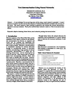
2 Loop Invariants Informally, an invariant is a property that always holds for (a part of) the program. The notion of invariants of computer programs has been an active research area from the early beginnings of computer science. A well-known instance are Hoare’s rules for reasoning about program correctness [37]. For the case of looping programs fragments, [37] refers to loop invariants, i.e., predicates that hold upon entry to a loop and after each iteration. As a result, loop invariants are guaranteed to hold immediately upon exit of the loop1 . For example, “p-a ≤ length(a)” is a loop invariant for the loop in Figure 1. Important types of loop invariants that are distinguished and used in this work are state invariants and transition invariants. Formally, a program can be represented as a transition system P = hS, I, Ri, where: – S is a set of states; – I ⊆ S is the set of initial states; – R ⊆ S × S is the transition relation. We use the relational composition operator ◦ which is defined for two binary relations Ri ⊆ S × S and Rj ⊆ S × S as Ri ◦ Rj := (s, s0 ) ∈ S × S

∃s00 ∈ S . (s, s00 ) ∈ Ri ∧ (s00 , s0 ) ∈ Rj .

To simplify the presentation, we also define R1 := R and Rn := Rn−1 ◦ R for any relation R : S × S. 1 Here we only consider structured loops or loops for which the exit condition is evaluated before an iteration has changed the state of any variables.

4


vi p=a; while(*p!=0){ if(*p==’/’) *p=0; p++; }

*p!=0

p=a

*p==’/’ *p!=’/’

*p==0

p++

*p=0

vo Fig. 1: The example of a program and its program graph

Note that a relation R is transitive if it is closed under relational composition, i.e., when R ◦ R ⊆ R. The reflexive and non-reflexive transitive closures of R are denoted as R∗ and R+ respectively. The set of reachable states is then defined as R∗ (I) := {s ∈ S ∃s0 ∈ I . (s0 , s) ∈ R∗ }. We now discuss two kinds of invariants, state invariants and transition invariants. For historical reasons, state invariants are often referred to simply as invariants; we will use the term “state invariant” when it is necessary to stress its difference to transition invariants. Definition 1 (State Invariant) A state invariant V for program P represented by a transition system hS, I, Ri is a superset of the reachable state space, i.e., R∗ (I) ⊆ V . In contrast to state invariants that represent the safety class of properties, transition invariants, introduced by Podelski and Rybalchenko [49], enable reasoning about liveness properties and, in particular, about program termination. Definition 2 (Transition Invariant [49]) A transition invariant T for program P represented by a transition system hS, I, Ri is a superset of the transitive closure of R restricted to the reachable state space, i.e., R+ ∩ (R∗ (I) × R∗ (I)) ⊆ T . State and transition invariants can be used together during loop summarization to preserve both safety- and liveness-related semantics of a loop in its abstraction. Our experiments with a static analyser tailored to buffer overflows focus on state invariants, while our experiments with termination analysis mainly use transition invariants.

3 Loop Summarization with State Invariants Algorithm 1 presents an outline of loop summarization. The function Summarize traverses the control-flow graph of the program P and calls itself recursively for each block with nested loops. If a block is a loop without nested loops, it is summarized using the function SummarizeLoop and the resulting summary replaces the original loop in P 0 . Thereby, outer loops also become loop-free, which enables further progress.


5

Algorithm 1: Routines of loop summarization Summarize(P ) input: program P output: Program summary begin foreach Block B in ControlFlowGraph(P ) do if B has nested loops then B :=Summarize(B) else if B is a single loop then B :=SummarizeLoop(B) endif 11 end foreach 12 return P 13 end 1 2 3 4 5 6 7 8 9 10

14 15 16 17 18 19 20 21 22

SummarizeLoop(L) input: Single-loop program L (over variable set X) output: Loop summary begin I := > foreach Candidate C in PickInvariantCandidates(L) do if IsStateInvariant(L, C) then I := I ∧ C endif 23 end foreach 24 return “X pre := X; havoc(X); assume(I(X pre ) =⇒ I(X));” 25 end 26 27 28 29 30 31

IsStateInvariant(L, C) input: Single-loop program L (over variable set X), invariant candidate C output: TRUE if C is an invariant for L; FALSE otherwise begin return Unsat(¬(L(X, X 0 ) ∧ C(X) ⇒ C(X 0 ))) end

The function SummarizeLoop computes the summaries. A very imprecise over-approximation is to replace a loop with a program fragment that “havocs” the state by setting all variables that are (potentially) modified during loop execution to non-deterministic values. To improve the precision of these summaries, we strengthen them by means of (partial) loop invariants. SummarizeLoop has two subroutines that are related to invariant discovery: PickInvariantCandidates, which returns a set of “invariant candidates” depending on an abstract interpretation selected for the loop and IsStateInvariant, which establishes whether a candidate is an actual loop invariant (a state invariant in this case). Note that this summarization algorithm only uses state invariants and does not take loop termination into account. State invariants over-approximate the set

6


of states that a loop can reach but do not provide any information about the progress of the loop. Thus, the summaries computed by the algorithm are always terminating program fragments. The abstraction is a sound over-approximation, but it may be too coarse for programs that contain unreachable paths. We address this issue in Section 5.

4 Summarization using Symbolic Abstract Transformers In the following subsections we formally describe the steps of our summarization approach. We first present necessary notation and define summarization as an over-approximation of a code fragment. Next, we show that a precise summary can be computed for a loop-free code fragment, and we explain how a precise summary of a loop body is used to obtain information about the computations of the loop. Finally, we give a bottom-up summarization algorithm applicable to arbitrary programs.

4.1 Abstract interpretation To formally state the summarization algorithm and prove its correctness we rely on abstract interpretation [22]. It constructs an abstraction of a program using values from an abstract domain by iteratively applying the instructions of a program to abstract values until a fixpoint is reached. Formally: Definition 3 A program graph is a tuple G = hPL, E, pli , plo , L, Ci, where – – – –

PL is a finite non-empty set of vertices called program locations; pli ∈ PL is the initial location; plo ∈ PL is the final location; E ⊆ PL × PL is a non-empty set of edges; E ∗ denotes the set of paths, i.e., the set of finite sequences of edges; – L is a set of elementary commands; – C : E → L associates a command with each edge.

A program graph is often used as an intermediate modeling structure in program analysis. In particular, it is used to represent the control-flow graph of a program. Example 1 To demonstrate the notion of a program graph we use the program fragment in Figure 1 as an example. On the left-hand side, we provide the program written in the programming language C. On the right-hand side, we depict its program graph. Let S be the set of states, i.e., the set of valuations of program variables. The ˙ A, set of commands L consists of tests LT and assignments LA , i.e., L = LT ∪L where: – a test q ∈ LT is a predicate over S (q ⊆ S); – an assignment e ∈ LA is a map from S to S.


7

A program P is then formalized as the pair hS, Gi, where S is the set of states and G is a program graph. We write L∗ for the set of sequences of commands. Given a program P , the set paths(P ) ⊆ L∗ contains the sequence C(e1 ), . . . , C(en ) for every he1 , .., en i ∈ E ∗ . The (concrete) semantics of a program is given by the pair hA, τ i, where: – A is the set of assertions of the program, where each assertion p ∈ A is a predicate over S (p ⊆ S); A(⇒, false, true, ∨, ∧) is a complete Boolean lattice; – τ : L → (A → A) is the predicate transformer. ˆ ti, where Aˆ is a complete lattice of the An abstract interpretation is a pair hA, ˆ ˆ is a predicate transformer. Note that form A(v,⊥, >, t, u), and t : L → (Aˆ → A) hA, τ i is a particular abstract interpretation called the concrete interpretation. In the following, we assume that for every command c ∈ L, the function t(c) (predicate transformer for command c) is monotone (which is the case for all natural predicate transformers). Given a predicate transformer t, the function ˆ is recursively defined as follows: t˜ : L∗ → (Aˆ → A) t˜(p)(φ) =

φ if p is empty t˜(e)(t(q)(φ)) if p = q; e for a q ∈ L, e ∈ L∗ .

Example 2 We continue using the program in Figure 1. Consider an abstract domain where abstract state is a four-tuple hpa , za , sa , la i. The first member, pa is the offset of the pointer p from the base address of the array a (i.e., p − a in our example), the Boolean za holds if a contains the zero character, the Boolean sa holds if a contains the slash character, la is the index of the first zero character if present. The predicate transformer t is defined as follows: t(p = a)(φ) = φ[pa := 0] for any assertion φ; t(∗p ! = 0)(φ) = φ ∧ (pa 6= la ) for any assertion φ; t(∗p == 0)(φ) = φ ∧ za ∧ (pa ≥ la ) for any assertion φ; t(∗p ==0 /0 )(φ) = φ ∧ sa for any assertion φ; t(∗p ! =0 /0 )(φ) = φ for any assertion φ; φ[za := true, la := pa ] if φ ⇒ (pa < la ) t(∗p = 0)(φ) = φ[za := true] otherwise; t(p++)(φ) = φ[pa := pa + 1] for any assertion φ. (We used φ[x := v] to denote an assertion equal to φ apart from the variable x that takes value v.) ˆ ti and an element φ ∈ A, ˆ Given a program P , an abstract interpretation hA, we define the Merge Over all Paths MOP P (t, φ) as MOP P (t, φ) :=

G

t˜(π)(φ) .

π∈paths(P )

ˆ Given two complete lattices A(v, ⊥, >, t, u) and Aˆ0 (v0 , ⊥0 , >0 , t0 , u0 ), the pair 0 ˆ ˆ of functions hα, γi, with α : A → A and γ : Aˆ0 → Aˆ is a Galois connection iff α and γ are monotone and satisfy: for all φ ∈ Aˆ : φ v γ(α(φ)) for all φ0 ∈ Aˆ0 : α(γ(φ0 )) v0 φ0 .

8


ˆ ti is a correct over-approximation of the conAn abstract interpretation hA, crete interpretation hA, τ i iff there exists a Galois connection hα, γi such that for all φ ∈ Aˆ and p ∈ A, if p ⇒ γ(φ), then α(MOP P (τ, p)) v MOP P (t, φ) (i.e., MOP P (τ, p) ⇒ γ(MOP P (t, φ))).

4.2 Computing Abstract Transformers In order to implement abstract interpretation for a given abstract domain, an algorithmic description of the abstract predicate transformer t(p) for a specific command p ∈ L is required. These transformers are frequently hand-coded for a given programming language and a given domain. Reps et al. describe an algorithm that computes the best possible (i.e., most precise) abstract transformer for a given finite-height abstract domain automatically [52]. Graf and Sa¨ıdi’s algorithm for constructing predicate abstractions [30] is identified as a special case. The algorithm presented by Reps et al. has two inputs: a formula Fτ (q) , which represents the concrete semantics τ (q) of a command q ∈ L symbolically, and ˆ It returns the image t(q)(φ) of the predicate transformer an assertion φ ∈ A. t(q). The formula Fτ (q) is passed to a decision procedure, which is expected to provide a satisfying assignment to the variables. The assignment represents one concrete transition (p, p0 ) ∈ A×A. The transition is abstracted into a pair (φ, φ0 ) ∈ ˆ and a blocking constraint is added to remove this satisfying assignment. Aˆ × A, The algorithm iterates until the formula becomes unsatisfiable. An instance of the algorithm for the case of predicate abstraction is the implementation of SatAbs described in [15]. SatAbs uses a propositional SAT-solver as decision procedure for bit-vector arithmetic. The procedure is worst-case exponential in the number of predicates, and thus, alternatives have been explored. In [42, 39] a symbolic decision procedure generates a symbolic formula that represents the set of all solutions. In [43], a first-order formula is used and the computation of all solutions is carried out by an SMT-solver. In [9], a similar technique is proposed where BDDs are used in order to efficiently deal with the Boolean component of Fτ (q) .

4.3 Abstract summarization The idea of summarization is to replace a code fragment, e.g., a procedure of the program, by a summary, which is a representation of the fragment. Computing an exact summary of a program (fragment) is undecidable in the general case. We therefore settle for an over-approximation. We formalize the conditions the summary must fulfill in order to have a semantics that over-approximates the original program. We extend the definition of a correct over-approximation (from Section 4.1) to programs. Given two programs P and P 0 , we say that P 0 is a correct over-approximation of P iff for all p ∈ A(⇒, false, true, ∨, ∧), M OPP (τ, p) ⇒ M OPP 0 (τ, p). Definition 4 (Abstract Summary) Given a program P , and an abstract interˆ ti with a Galois connection hα, γi with hA, τ i, we denote the abstract pretation hA, summary of P by SumhA,ti ˆ (P ). It is defined as the program hU, Gi, where U denotes the universe of program variables and G = h{vi , vo }, {hvi , vo i}, vi , vo , {a}, Ci


9

and {a} together with C(hvi , vo i) = a, where a is a new (concrete) command such that τ (a)(p) = γ(MOP P (t, α(p))). ˆ ti is a correct over-approximation of hA, τ i, the abstract sumLemma 1 If hA, mary SumhA,ti (P ) is a correct over-approximation of P . ˆ Proof Let P 0 = SumhA,ti ˆ (P ). For all p ∈ A, M OPP (τ, p)) ⇒ γ(M OPP (t, α(p)))[by def. of correct over-approx.] = τ (a)(p)[by Definition 4] = M OPP 0 (τ, p) [MOP over a single-command path]. The following sections discuss our algorithms for computing abstract summaries. The summarization technique is first applied to particular fragments of the program, specifically to loop-free (Section 4.4) and single-loop programs (Section 4.5). In Section 4.6, we use these procedures as subroutines to obtain the summarization of an arbitrary program. We formalize code fragments as program sub-graphs. Definition 5 Given two program graphs G = hV, E, vi , vo , L, Ci and G0 = hV 0 , E 0 , vi0 , vo0 , L0 , C 0 i, G0 is a program sub-graph of G iff V 0 ⊆ V , E 0 ⊆ E, and C 0 (e) = C(e) for every edge e ∈ E 0 . 4.4 Summarization of loop-free programs Obtaining MOP P (t, φ) is as hard as assertion checking on the original program. Nevertheless, there are restricted cases where it is possible to represent MOP P (t, φ) using a symbolic predicate transformer. Let us consider a program P with a finite number of paths, in particular, a program whose program graph does not contain any cycles. A program graph G = hV, E, vi , vo , L, Ci is loop-free iff G is a directed acyclic graph. In the case of a loop-free program P , we can compute a precise (not abstract) summary by means of a formula FP that represents the concrete behavior of P . This formula is obtained by converting P to static single assignment (SSA) form, whose size is linear in the size of P (this step is beyond the scope of this work; see [14] for details). Example 3 We continue the running example (Fig. 1). The symbolic transformer of the loop body P 0 is represented by: ((∗p =0 /0 ∧ a0 = a[∗p = 0]) ∨ (∗p 6=0 /0 ∧ a0 = a)) ∧ (p0 = p + 1) . Recall the abstract domain from Ex. 2. We can deduce that: 1. if m < n, then MOP P 0 (t, (pa = m∧za ∧(la = n)∧¬sa )) = (pa = m+1∧za ∧la = n ∧ ¬sa ) 2. MOP P 0 (t, za ) = za . This example highlights the generic nature of our technique. For instance, case 1 of the example cannot be obtained by means of predicate abstraction because it requires an infinite number of predicates. Also, the algorithm presented in [52] cannot handle this example because assuming the string length has no a-priori bound, the lattice of the abstract interpretation has infinite height.

10


4.5 Summarization of single-loop programs We now consider a program that consists of a single loop.

Definition 6 A program P = hU, Gi is a single-loop program iff G = hV, E, vi , vo , L, Ci and there exists a program sub-graph G0 and a test q ∈ LT such that q vo

vi

– G0 = hV 0 , E 0 , vb , vi , L0 , C 0 i with – V 0 = V \ {vo }, – E 0 = E \ {hvi , vo i, hvi , vb i}, – L0 = L \ q, – C 0 (e) = C(e) for all e ∈ E 0 , – G0 is loop-free. – C(hvi , vb i) = q, C(hvi , vo i) = q.

q vb G0

We first record the following simple lemma.

ˆ ti, if Lemma 2 Given a loop-free program P , and an abstract interpretation hA, MOP P (t, ψ) v ψ, then, for all repetitions of loop-free paths of a program P , i.e., for all π ∈ (paths(P ))∗ , t˜(π)(ψ) v ψ. Proof If MOP P (t, ψ) = π∈paths(P ) t˜(π)(ψ) v ψ, then, for all paths π ∈ paths(P ), t˜(π)(ψ) v ψ. Thus, by induction on repetitions of loop-free paths, for all paths π ∈ (paths(P ))∗ , t˜(π)(ψ) v ψ. F

The following can be seen as the “abstract interpretation analog” of Hoare’s rule for while loops.

Theorem 1 Given a single-loop program P with guard q and loop body P 0 , and an ˆ ti, let ψ be an assertion satisfying MOP P 0 (t, t(q)(ψ)) abstract interpretation hA, ˆ tψ i be a new abstract interpretation s.t. v ψ and let hA,

MOP P (tψ , φ) =

t(q)(ψ) if φ v ψ > elsewhere.

ˆ ti is a correct over-approximation, then hA, ˆ tψ i is also a correct over-approxIf hA, imation.


11

Proof If φ v ψ, ˆ ti is a correct over-approximation] α(MOP P (τ, p)) v MOP P (t, p) [hA, G = t˜(π)(φ) [by definition of MOP ] π∈paths(P )

v

G

t˜(π)(ψ)

[φ v ψ]

π∈paths(P )

t˜((π 0 ; q)∗ )(ψ) [P is a single-loop program]

G

=

π∈(q;π 0 )∗ ,π 0 ∈paths(P 0 )

t˜((q)∗ )(t˜((π 0 )∗ )(ψ))

G

=

[by definition of t˜]

π∈(q;π 0 )∗ ,π 0 ∈paths(P 0 )

G

v t(q)(

t˜((π 0 )∗ )(ψ))

[t is monotone]

π∈(q;π 0 )∗ ,π 0 ∈paths(P 0 )

v t(q)(ψ)

[by Lemma 2]

Otherwise, trivially α(MOP P (τ, p)) v > = MOP P (tψ , φ). In other words, if we apply the predicate transformer of the test q and then the transformer of the loop body P 0 to the assertion ψ, and we obtain an assertion at least as strong as ψ, then ψ is a state invariant of the loop. If a stronger assertion φ holds before the loop, the predicate transformer of q applied to φ holds afterwards. Theorem 1 gives rise to a summarization algorithm. Given a program fragment and an abstract domain, we heuristically provide a set of formulas, which encode that a (possibly infinite) set of assertions ψ are invariant (for example, x0 = x encodes that every ψ defined as x = c, with c a value in the range of x, is an invariant). We apply a decision procedure to check if the formulas are unsatisfiable (see IsStateInvariant(L,C) in Algorithm 1). The construction of the summary is then straightforward: given a single-loop ˆ ti, and a state invariant ψ for the loop program P , an abstract interpretation hA, ˆ tψ i be the abstract interpretation as defined in Theorem 1. We denote body, let hA, ˆ the summary SumhA,t ˆ ψ i (P ) by SlS(P, A, tψ ) (Single-Loop Summary). ˆ ti is a correct over-approximation of hA, τ i, then SlS(P, A, ˆ Corollary 1 If hA, tψ ) is a correct over-approximation of P . Example 4 We continue the running example from Figure 1. Recall the abstract domain in Ex. 2. Let P 0 denote the loop body of the example program and let q denote the loop guard. By applying the symbolic transformer from Ex. 3, we can check that the following conditions hold: 1. MOP P 0 (t, t(q)(φ)) v φ for any assertion ((pa ≤ la ) ∧ za ∧ ¬sa ). 2. MOP P 0 (t, t(q)(φ)) v φ for the assertion za . Thus, we summarize the loop with the following predicate transformer: (za → za0 ) ∧ (((pa ≤ la ) ∧ za ∧ ¬sa ) → ((p0a = la0 ) ∧ za0 ∧ ¬s0a )) .

12


Algorithm 2: Arbitrary program summarization 1 Summarize(P )

2 3 4 5 6 7 8 9 10 11

12 13

14 15 16 17 18 19

input : program P = hU, Gi output: over-approximation P 0 of P begin hT, >i :=sub-graph dependency tree of P ; Pr := P ; for each G0 such that G > G0 do hU, G00 i:=Summarize(hU, G0 i); Pr := Pr where G0 is replaced with G00 ; update hT, >i; end for if Pr is a single loop then ˆ ti := choose abstract interpretation for Pr ; hA, /* Choice of abstract interpretation defines set of candidate assertions ψ, which are checked to hold in the next step. */ ψ := test state invariant candidates for t on Pr ; ˆ tψ ); P 0 := SlS(Pr , A, /* Those ψ that hold on Pr form the single-loop summary (SlS). */ endif else /* Pr is loop-free */ P 0 := SumhA,τ i (Pr ); endif return P 0 end

4.6 Summarization for programs with multiple loops We now describe an algorithm for over-approximating a program with multiple loops that are possibly nested. Like traditional algorithms (e.g., [56]), the dependency tree of program fragments is traversed bottom-up, starting from the leaves. The code fragments we consider may be function calls or loops. We treat function calls as arbitrary sub-graphs (see Definition 5) of the program graph, and do not allow recursion. We support irreducible graphs using loop simulation [2]. Specifically, we define the sub-graph dependency tree of a program P = hU, Gi as the tree hT, >i, where – – – – –

the set of nodes of the tree are program sub-graphs of G; for G1 , G2 ∈ T , G1 > G2 iff G2 is a program sub-graph of G1 with G1 6= G2 ; the root of the tree is G; every leaf is a loop-free or single-loop sub-graph; every loop sub-graph is in T .

Algorithm 2 takes a program as input and computes its summary by following the structure of the sub-graph dependency tree (Line 3). Thus, the algorithm is


13

called recursively on the sub-program until a leaf is found (Line 5). If it is a single loop, an abstract domain is chosen (Line 11) and the loop is summarized as described in Section 4.5 (Line 13). If it is a loop-free program, it is summarized with a symbolic transformer as described in Section 4.4 (Line 16). The old subprogram is then replaced with its summary (Line 7) and the sub-graph dependency tree is updated (Line 8). Eventually, the entire program is summarized. Theorem 2 Summarize(P ) is a correct over-approximation of P . Proof We prove the theorem by induction on the structure of the sub-graph dependency tree. In the first base case (Pr is loop-free), the summary is precise by construction and is thus a correct over-approximation of P . In the second base case (Pr is a single loop), by hypothesis, each abstract interpretation chosen at Line 11 is a correct over-approximation of the concrete interpretation. Thus, if P is a single-loop or a loop-free program, P 0 is a correct over-approximation of P (resp. by Theorem 1 and by definition of abstract summary). In the inductive case, we select a program subgraph G0 and we replace it with G00 , where hU, G00 i=Summarize(hU, G0 i). Through the induction hypothesis, we obtain that hU, G00 i is a correct over-approximation of hU, G0 i. Thus, for all p ∈ A, MOP hU,G0 i (τ, p) ⇒ MOP hU,G00 i (τ, p). Note that G00 contains only a single command g. We want to prove that for all p ∈ A, MOP P (τ, p) ⇒ MOP P 0 (τ, p) (for readability, we replace the subscript “(πi ; πg ; πf ) ∈ paths(P ), πg ∈ paths(hU, G0 i), and πi ∩ G0 = ∅” with ∗ and “π ∈ paths(P ), and π ∩ G0 = ∅” with ∗∗): G

MOP P (τ, p) =

τ˜(π)(p)

[by definition of MOP ]

π∈paths(P )

=

G

τ˜(πf )(˜ τ (πg )(˜ τ (πi )(p))) ∪

∗

G

τ˜(π)(p)

⇒

G

=

G

τ˜(πf )(MOP hU,G00 i (˜ τ , (˜ τ (πi )(p)))) ∪

∗

G

τ˜(π)(p) [G00 is an over-approx.]

∗∗

τ˜(πf )(MOP hU,(G00 ;πi )i (τ, p)) ∪

∗

=

[G0 is a subgraph]

∗∗

G

τ˜(π)(p)


∗∗

G

MOP π[g/πg ] (τ, p)

[by induction on length of paths]

π∈paths(P )

=

G

MOP π (τ, p)

[by definition of π 0 ]

π∈paths(P 0 )

= MOP π0 (τ, P )


The precision of the over-approximation is controlled by the precision of the symbolic transformers. However, in general, the computation of the best abstract transformer is an expensive iterative procedure. Instead, we use an inexpensive syntactic procedure for loop-free fragments. Loss of precision only happens when summarizing loops, and greatly depends on the abstract interpretation chosen in Line 11.

14


Note that Algorithm 2 does not limit the selection of abstract domains to any specific type of domain, and that it does not iterate the predicate transformer on the program. Furthermore, this algorithm allows for localization of the summarization procedure, as a new domain may be chosen for every loop. Once the domains are fixed, it is also straightforward to monitor the progress of the summarization, as the number of loops and the cost of computing the symbolic transformers are known—another distinguishing feature of our algorithm. The summarization can serve as an over-approximation of the program. It can be trivially analyzed to prove unreachability, or equivalently, to prove assertions.

4.7 Leaping counterexamples Let P 0 denote the summary of the program. The program P 0 is a loop-free sequence of symbolic summaries for loop-free fragments and loop summaries. A counterexample for an assertion in P 0 follows this structure: for loop-free program fragments, it is identical to a concrete counterexample. Upon entering a loop summary, the effect of the loop body is given as a single transition in the counterexample: we say that the counterexample leaps over the loop. Example 5 Consider the summary from Ex. 4. Suppose that in the initial condition, the buffer a contains a null terminating character in position n and no 0 /0 character. If we check that, after the loop, pa is greater than the size n, we obtain a counterexample with p0a = 0, p1a = n. The leaping counterexample may only exist with respect to the abstract interpretations used to summarize the loops, i.e., the counterexample may be spurious in the concrete interpretation. Nevertheless, leaping counterexamples provide useful diagnostic feedback to the programmer, as they show a (partial) path to the violated assertion, and contain many of the input values the program needs to violate the assertion. Furthermore, spurious counterexamples can be eliminated by combining our technique with counterexample-guided abstraction refinement, as we have an abstract counterexample. Other forms of domain refinement are also applicable.

5 Termination Analysis using Loop Summarization In this section we show how to employ loop summarization with transition invariants to tackle the problem of program termination.

5.1 The termination problem The termination problem (also known as the uniform halting problem) is has roots in Hilbert’s Entscheidungsproblem and can be formulated as follows: In finite time, determine whether a given program always finishes running or could execute forever.


15

Undecidability of this problem was shown by Turing [57]. This result sometimes gives rise to the belief that termination of a given program can never be proven. In contrast, numerous algorithms that prove termination of many realistic classes of programs have been published, and termination analysis now is at a point where industrial application of termination proving tools for specific programs is feasible. One key fact underlying these methods is that termination may be reduced to the construction of well-founded ranking relations [58]. Such a relation establishes an order between the states of the program by ranking each of them, i.e., by assigning a natural number to each state such that for any pair of consecutive states si , si+1 in any execution of the program, the rank decreases, i.e., rank(si+1 ) < rank(si ). The existence of such an assignment ensures well-foundedness of the given set of transitions. Consequently, a program is terminating if there exists a ranking function for every program execution. Podelski and Rybalchenko proposed disjunctive well-foundedness of transition invariants [49] as a means to improve the degree of automation of termination provers. Based on this discovery, the same authors together with Cook gave an algorithm to verify program termination using iterative construction of transition invariants—the Terminator algorithm [17, 18]. This algorithm exploits the relative simplicity of ranking relations for a single path of a program. It relies on a safety checker to find previously unranked paths of a program, computes a ranking relation for each of them individually, and disjunctively combines them in a global (disjunctively well-founded) termination argument. This strategy shifts the complexity of the problem from ranking relation synthesis to safety checking, a problem for which many efficient solutions exist (mainly by means of reachability analysis based on Model Checking). The Terminator algorithm was successfully implemented in tools (e.g., the Terminator [18] tool, ARMC [50], SatAbs [21]) and applied to verify industrial code, most notably, Windows device drivers. However, it has subsequently become apparent that the safety check is a bottleneck of the algorithm, consuming up to 99% of the run-time [18, 21] in practice. The runtime required for ranking relation synthesis is negligible in comparison. A solution to this performance issue is Compositional Termination Analysis (CTA) [40]. This method limits path exploration to several iterations of each loop of the program. Transitivity (or compositionality) of the intermediate ranking arguments is used as a criterion to determine when to stop the loop unwinding. This allows for a reduction in run-time, but introduces incompleteness since a transitive termination argument may not be found for each loop of a program. However, experimental evaluation on Windows device drivers confirmed that this case is rare in practice. The complexity of the termination problem together with the observation that most loops have, in practice, (relatively) simple termination arguments suggests the use of light-weight static analysis for this purpose. In particular, we propose a termination analysis based on the loop summarization algorithm described in Section 3. We build a new technique for termination analysis by 1) employing an abstract domain of (disjunctively well-founded) transition invariants during summarization and 2) using a compositionality check as a completeness criterion for the discovered transition invariant.

16


5.2 Formalism for reasoning about termination As described in Section 2, we represent a program as a transition system P = hS, I, Ri, where: – S is a set of states; – I ⊆ S is the set of initial states; – R ⊆ S × S is the transition relation. We also make use of the notion of (disjunctively well-founded) transition invariants (Definition 2, page 4) introduced by Podelski and Rybalchenko [49]. Definition 7 (Well-foundedness) A relation R is well-founded (wf.) over S if for any non-empty subset of S, there exists a minimal element (with respect to R), i.e., ∀X ⊆ S . X 6= ∅ =⇒ ∃m ∈ X, ∀s ∈ X, (s, m) ∈ / R. The same does not hold for the weaker notion of disjunctive well-foundedness. Definition 8 (Disjunctive Well-foundedness [49]) A relation T is disjunctively well-founded (d.wf.) if it is a finite union T = T1 ∪ · · · ∪ Tn of well-founded relations. The main result of the work [49] concludes program termination from the existence of disjunctively well-founded transition invariant. Theorem 3 (Termination [49]) A program P is terminating iff there exists a d.wf. transition invariant for P . This result is applied in the Terminator2 algorithm [18], which automates construction of d.wf. transition invariants. It starts with an empty termination condition T = ∅ and queries a safety checker for a counterexample—a computation that is not covered by the current termination condition T . Next, a ranking relation synthesis algorithm is used to obtain a termination argument T 0 covering the transitions in the counterexample. The termination argument is then updated as T := T ∪ T 0 and the algorithm continues to query for counterexamples. Finally, either a complete (d.wf.) transition invariant is constructed or there does not exist a ranking relation for some counterexample, in which case the program is reported as non-terminating.

5.3 Compositional termination analysis Podelski and Rybalchenko [49] remarked an interesting fact regarding the compositionality (transitivity) of transition invariants: If T is transitive, it is enough to show that T ⊇ R instead of T ⊇ R+ to conclude termination, because a compositional and d.wf. transition invariant is well-founded, since it is an inductive transition invariant for itself [49]. Therefore, compositionality of a d.wf. transition invariant implies program termination. To comply with the terminology in the existing literature, we define the notion of compositionality for transition invariants as follows: 2 The Terminator algorithm is referred to as Binary Reachability Analysis (BRA), though BRA is only a particular technique to implement the algorithm (e.g., [21]).


17

Definition 9 (Compositional Transition Invariant [49, 40]) A d.wf. transition invariant T is called compositional if it is also transitive, or equivalently, closed under composition with itself, i.e., when T ◦ T ⊆ T . This useful property did not find its application in termination analysis until 2010. To understand its value we need to look closer at the transitive closure of program’s transition relation R. The safety checker in the Terminator algorithm verifies that a candidate transition invariant T indeed includes R+ restricted to the reachable states. Note that the (non-reflexive) transitive closure of R is essentially an unwinding of program loops: R+ = R ∪ (R ◦ R) ∪ (R ◦ R ◦ R) ∪ . . . =

∞ [

Ri .

i=1

Thus, instead of searching for a d.wf. transition invariant that is a superset of R+ , we can therefore decompose the problem into a series of smaller ones. We can consider a series of loop-free programs in which R is unwound k times, i.e., the program that contains the transitions in R1 ∪ . . . ∪ Rk . As was shown in [40], Sk if there is a d.wf. Tk with j=1 Rj ⊆ Tk and Tk is also transitive, then Tk is a compositional transition invariant for P . This idea results in an algorithm that constructs d.wf. relations Ti for incrementally deep unwindings of P until it finally finds a transitive Tk , which proves termination of P . In [40], this algorithm was named Compositional Termination Analysis (CTA).

5.4 From Terminator via CTA to a light-weight static analysis Terminator is a complete algorithm (relative to completeness of the ranking procedure). Note that CTA is not even complete relative to the completeness of the ranking procedure for terminating programs even if they are finite-state. This is due to the fact that T is not guaranteed to ever become transitive, even if it contains R+ . The Terminator strategy can be seen as a “proof by construction”: it explicitly builds the valid terminating argument for every path in a program. CTA combines “proof by construction” with a “proof by induction”: it first tries to construct a base step and then check the inductiveness. Inductive proofs are hard to find, and the implementation reported in [40] can only compute very simple inductive arguments. However, as it was shown in [40], for loops in industrial applications such as Windows device drivers, that CTA performs considerably better than Terminator. This observation suggests an even more light-weight proof strategy—from a mix of “proof by construction” with “proof by induction” to a pure “proof by induction”: we propose to replace ranking synthesis-based transition invariant discovery with abstract domain-based transition invariant discovery. Instead of a complex base case, we “guess” several variants of the loop using lightweight static analysis methods and then check if the inductive argument happens to hold as well. This method is of course incomplete, but avoids expensive path enumeration inside the safety checker. We apply a variant of our loop summarization algorithm with specific relational domains for this purpose.

18


5.5 Loop summarization with transition invariants We introduce a method that allows transition invariants to be included for strengthening of loop summaries. This increases the precision of the summaries by allowing loop termination to be taken into account. According to Definition 2, a binary relation T is a transition invariant for a program P if it contains R+ (restricted to the reachable states). Note, however, that transitivity of T is also a sufficient condition when T is only a superset of R: Theorem 4 A binary relation T is a transition invariant for the program hS, I, Ri if it is transitive and R ⊆ T . Proof From transitivity of T it follows that T + ⊆ T . Since R ⊆ T it follows that R+ ⊆ T . This simple fact allows for an integration of transition invariants into the loop summarization framework by a few adjustments to the original algorithm. Consider line 19 of Algorithm 1 (page 5), where candidate invariants are selected. Clearly, we need to allow selection of transition invariants here, i.e., invariant candidates now take the relational form C(X, X 0 ), where X 0 is the post-state of a single iteration of L. What follows is a check for invariance of C over L(X, X 0 ), i.e., a single unwinding of the loop. Consider the temporary (sub-)program hS, S, Li to represent the execution of the loop from a non-deterministic entry state. A transition invariant for this program is required to cover L+ , which, according to Theorem 4, is implied by L ⊆ C and transitivity of C. The original invariant check in IsTransitionInvariant establishes L ⊆ C, when the check for unsatisfiability receives the more general formula L(X, X 0 ) ∧ C(X, X 0 ) as a parameter. The summarization procedure furthermore requires a slight change to include a check for compositionality. The resulting procedure is Algorithm 3.

5.6 Termination checks The changes to the summarization algorithm allow for termination checks during summarization through application of Theorem 3, which requires a transition invariant to be disjunctively well-founded. This property may be established by allowing only disjunctively well-founded invariant candidates, or it may be checked by means of decision procedures (e.g., SMT solvers where applicable). According to Definition 8, the well-foundedness of each of the disjuncts of a candidate relation T must be established in order to ensure that it is d.wf. This can be done by an explicit encoding of the well-foundedness criteria given in Definition 7. However, the resulting formula contains quantifiers. As a consequnce, the obtained decision problem is frequently beyond the capabilities of state-of-theart solvers.


19

Algorithm 3: Loop summarization with transition invariants. 1 2 3 4 5 6 7 8 9

SummarizeLoop-TI(L) input: Single-loop program L with a set of variables X output: Loop summary begin T := > foreach Candidate C in PickInvariantCandidates(L) do if IsTransitionInvariant(L, C) ∧ IsCompositional(C) then T := T ∧ C endif 10 end foreach 11 return “X pre := X; havoc(X); assume(T (X pre , X));” 12 end 13 IsTransitionInvariant(L, C) 14 input: Single-loop program L (with entry state X and post-iteration state 15 16 17 18

X 0 ), invariant candidate C output: TRUE if C is a transition invariant for L; FALSE otherwise begin return Unsat(¬(L(X, X 0 ) ∧ C(X, X 0 ) ⇒ C(X, X 0 ))) end

19 20 21 22 23 24

IsCompositional(C) input: Invariant candidate C(X, X 0 ) output: TRUE if C is compositional; FALSE otherwise begin return Unsat(¬ C(X, Y ) ∧ C(Y, X 0 ) ⇒ C(X, X 0 ) ) end

5.7 The difference between Terminator, CTA and loop summarization-based termination The complexity of establishing well-foundedness of a transition invariant hints at the explanation of a major difference between our new algorithm and Terminator/CTA. The latter construct the transition invariant using the abstractionrefinement loop such that it is already disjunctively well-founded, while we allow any transition invariant to be discovered, though, later it needs to be checked for well-foundedness. Note that even if the discovered transition invariant is not wellfounded, it is still a valid transition invariant and can therefore be used to improve the precision of summaries. However, the research in size-change termination for functional languages [5]3 suggests that a small set of templates for ranking relations is enough to cover many classes of programs. Besides, the expensive well-foundedness check can be completely omitted if we employ specialized abstract domains that produce only 3 We

discuss the relation of our method to size-change termination in Section 7.2.1.

20


well-founded candidates for transition invariants. This is the approach we take in the following section. Example 6 Consider the program in Figure 2. The symbolic transformer for the loop body is: φL := x0 = x + 1. Also consider the relation “>” for a pair x0 and x as a candidate relation Tc . Tc is indeed a transition invariant if the following formula is unsatisfiable:

int x = 0 ; while ( x x) . The formula is UNSAT, i.e., the invariant holds, and x0 > x is added to the symbolic transformer as a transition invariant. Since the relation is compositional and d.wf. (we explain the reason for this later), the loop is marked as terminating.

5.8 Invariant candidate selection We now propose a set of specialized candidate relations, which we find useful in practice, as demonstrated in the following section. We focus on transition invariants for machine-level integers (i.e., finite integers with overflows) for a bit-precise analysis of programs implemented in low-level languages such as ANSI-C. In contrast to other work on termination proving with abstract domains (e.g., [6]), we do not aim for general domains like Octagons and Polyhedra. Although fast in computation, they are not designed for termination and d.wf. and compositionality checks for them can be costly. Instead we focus on domains that – generate few, relatively simple candidate relations; – allow for efficient d.wf. and compositionality checks. Arithmetic operations on machine-level integers usually allow overflows, e.g., the instruction i = i+1 for a pre-state i = 2k −1 results in a post-state i0 = −2k−1 (when represented in two’s-complement). If termination of the loop depends on machine-level integers, establishing well-foundedness of a relation over it is not straightforward, as increasing/decreasing sequences of numbers of this kind can be affected by overflow/underflow. However, we can use the following theorem to simplify the discovery of a d.wf. transition invariant. Theorem 5 If T : K × K is a strict order relation for a finite set K ⊆ S and is a transition invariant for the program hS, I, Ri, then T is well-founded. Proof If T is a transition invariant, then for all pairs (k1 , k2 ) ∈ K × K. Thus, it is total over K. Non-empty finite totally-ordered sets always have a least element and, therefore, T is well-founded. The proof uses the fact that, when checking T for being a transition invariant, we implicitly enumerated all the pairs of pre- and post-states to discover if any of them violates the order. A total strict-order relation is also transitive, which allows for an alternative (stronger) criterion than Theorem 3:


21

Corollary 2 A program terminates if it has a transition invariant T that is also a finite strict-order relation. This corollary allows for a selection of invariant candidates that ensures (disjunctive) well-foundedness of transition invariants. An explicit check is therefore not required. An example of such a candidate appears in Example 6. Note that strictly ordered and finite transition invariants exist for many programs in practice: machine-level integers or strings of fixed length have a finite number of possible distinct pairs and strict natural or lexicographical orders are defined for them as well.

6 Experimental Evaluation This section first presents Loopfrog—a tool that implements loop summarization and serves as a basis for our experiments. Next, we evaluate the implementation to detect buffer overflows in ANSI-C programs. We finally demonstrate the applicability of loop summarization to termination analysis.

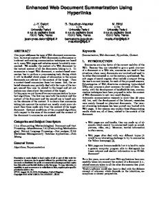
6.1 The Loopfrog tool The theoretical concept of symbolic abstract transformers is implemented and put to use by our tool Loopfrog. Its architecture is outlined in Figure 3. As input, Loopfrog receives a model file, extracted from software sources by Goto-CC4 . This model extractor features full ANSI-C support and simplifies verification of software projects that require complex build systems. It mimics the behavior of the compiler, and thus ‘compiles’ a model file using the original settings and options. Switching from compilation mode to verification mode is thus frequently achieved by changing a single option in the build system. As suggested by Figure 3, all other steps are fully automated. The resulting model contains a control flow graph and a symbol table, i.e., it is an intermediate representation of the original program in a single file. For calls to system library functions, abstractions containing assertions (pre-condition checks) and assumptions (post-conditions) are inserted. Note that the model also can contain the properties to be checked in the form of assertions (calls to the assert function). Preprocessing The model, instrumented with assertions, is what is passed to the first stage of Loopfrog. In this preprocessing stage, the model is adjusted in various ways to increase performance and precision. First, irreducible control flow graphs are rewritten according to an algorithm due to Ashcroft and Manna [2]. Like a compiler, Loopfrog inlines small functions, which increases the model size, but also improves the precision of subsequent analysis. Thereafter, it runs a field-sensitive pointer analysis. The information obtained this way is used to generate assertions over pointers, and to eliminate pointer variables in the program where possible. Loopfrog automatically adds assertions to verify the correctness of pointer operations, array bounds, and arithmetic overflows. 4 http://www.cprover.org/goto-cc/

22


ANSI-C Sources

Model Extractor

Preprocessing op

te nt ia li

nv ar ia nt s

lo

loops

is invariant?

su m

Verification Engine

Yes/No

aries

po

Loop Summarization

m

loop-free fragments

bo

dy

Abstract Domains

Verification Engine Loopfrog ‘SAFE’ or Leaping Counterexample

Fig. 3: Architecture of Loopfrog

Loop summarization Once the preprocessing is finished, Loopfrog starts to replace loops in the program with summaries. These are shorter, loop-free program fragments that over-approximate the original program behavior. To accomplish this soundly, all loops are replaced with a loop-free piece of code that “havocs” the program state, i.e., it resets all variables that may be changed by the loop to unknown values. Additionally, a copy of the loop body is kept, such that assertions within the loop are preserved. While this is already enough to prove some simple properties, much higher precision is required for more complex ones. As indicated in Fig. 3, Loopfrog makes use of predefined abstract domains to achieve this. Every loop body of the model is passed to a set of abstract domains, through each of which a set of potential invariants of the loop is derived (heuristically). The choice of the abstract domain for the loop summarization has a significant impact on the performance of the algorithm. A carefully selected domain generates fewer invariant candidates and thus speeds up the computation of a loop summary. The abstract domain has to be sufficiently expressive to retain enough of the semantics of the original loop to show the property.


#

Constraint

Meaning

1 2

ZTs Ls < Bs

3 4 5 6 7 8

0 ≤ i ≤ Ls 0≤i 0 ≤ i < Bs 0 ≤ i < Bs − k 0 < offset(p) ≤ Bs valid (p)

String s is zero-terminated Length of s (Ls ) is less than the size of the allocated buffer (Bs ) Bounds on integer variables i (i is non-negative, i is bounded by buffer size, etc.) k is an arbitrary integer constant. Pointer offset bounds Pointer p points to a valid object

23

Table 1: Examples of abstract domains tailored to buffer-overflow analysis.

Checking invariant candidates All potential invariants obtained from abstract domains always constitute an abstract (post-)state of a loop body, which may or may not be correct in the original program. To ascertain that a potential invariant is an actual invariant, Loopfrog makes use of a verification engine. In the current version, the symbolic execution engine of CBMC [14] is used. This engine allows for bit-precise, symbolic reasoning without abstraction. In our context, it always gives a definite answer, since only loop-free program fragments are passed to it. It is only necessary to construct an intermediate program that assumes a potential invariant to be true, executes a loop body once and then checks if the potential invariant still holds. If the verification engine returns a counterexample, we know that a potential invariant does not hold; in the opposite case it can be a loop invariant and it is subsequently added to a loop summary, since even after the program state is havoced, the invariant still holds. Loopfrog starts this process from an innermost loop, and thus there is never an intermediate program that contains a loop. In case of nested loops, the inner loop is replaced with a summary before the outer loop is analyzed. Owing to this strategy and the small size of fragments checked (only a loop body), small formulas are given to the verification engine and an answer is obtained quickly. Verifying the abstraction The result, after all loops have been summarized, is a loop-free abstraction of the input program. This abstract model is then handed to a verification engine once again. The verification time is much lower than that required for the original program, since the model does not contain loops. As indicated by Fig. 3, the verification engine used to check the assertions in the abstract model may be different from the one used to check potential invariants. In Loopfrog, we choose to use the same engine (CBMC).

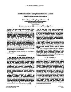
6.2 An abstract domain for safety analysis of string-manipulating programs In order to demonstrate the benefits of our approach to static analysis of programs with buffer overflows, the first experiments with Loopfrog were done with a set of abstract domains that are tailored to buffer-related properties. The constrains of the domains are listed in Table 1.

24


We also make use of string-related abstract domains instrumented into the model similar to the approach by Dor et al. [25]: for each string buffer s, a Boolean value zs and integers ls and bs are tracked. The Boolean zs holds if s contains the zero character within the buffer size bs . If so, ls is the index of the first zero character, otherwise, ls has no meaning. The chosen domains are instantiated according to variables occurring in the code fragment taken into account. To lower the number of template instantiations, the following simple heuristics can be used: 1. Only variables of appropriate type are considered (we concentrate on string types). 2. Indices and string buffers are combined in one invariant only if they are used in the same expression, i.e., we detect instructions which contain p[i] and build invariants that combine i with all string buffers pointed to by p. As shown in the next section these templates have proven to be effective in our experiments. Other applications likely require different abstract domains. However, new domain templates may be added quite easily: they usually can be implemented with less than a hundred lines of code.

6.3 Evaluation of loop summarization applied to static analysis of buffer-intensive programs In this set of experiments we focus on ANSI-C programs: the extensive buffer manipulations in programs of this kind often give rise to buffer overruns. We apply the domains from Table 1 to small programs collected in benchmarks suites and to real applications as well. All data was obtained on an 8-core Intel Xeon with 3.0 GHz. We limited the run-time to 4 hours and the memory per process to 4 GB. All experimental data, an in-depth description of Loopfrog, the tool itself, and all our benchmark files are available on-line for experimentation by other researchers5 . 6.3.1 Evaluation on the benchmark suites The experiments are performed on two recently published benchmark sets. The first one, by Zitser et al. [59], contains 164 instances of buffer overflow problems, extracted from the original source code of sendmail, wu-ftpd, and bind. The test cases do not contain complete programs, but only those parts required to trigger the buffer overflow. According to Zitser et al., this was necessary because the tools in their study were all either unable to parse the test code, or the analysis used disproportionate resources before terminating with an error ([59], pg. 99). In this set, 82 tests contain a buffer overflow, and the rest represent a fix of a buffer overflow. We use metrics proposed by Zitser et al. [59] to evaluate and compare the precision of our implementation. We report the detection rate R(d) (the percentage of correctly reported bugs) and the false positive rate R(f ) (the percentage of incorrectly reported bugs in the fixed versions of the test cases). The discrimination 5 http://www.cprover.org/loopfrog/


25

rate R(¬f |d) is defined as the ratio of test cases on which an error is correctly reported, while it is, also correctly, not reported in the corresponding fixed test case. Using this measure, tools are penalized for not finding a bug, but also for not reporting a fixed program as safe. The results of a comparR(d) R(f ) R(¬f |d) ison with a wide selection Loopfrog 1.00 0.38 0.62 of static analysis tools6 are =, 6=, ≤ 1.00 0.44 0.56 summarized in Table 2. AlInterval Domain 1.00 0.98 0.02 most all of the test cases inPolyspace 0.87 0.50 0.37 volve array bounds violations. Splint 0.57 0.43 0.30 Even though Uno, Archer and Boon 0.05 0.05 0 BOON were designed to detect Archer 0.01 0 0 these type of bugs, they hardly Uno 0 0 0 report any errors. BOON abstracts all string manipulaLoopfrog [41] 1.00 0.26 0.74 tion using a pair of inte=, 6=, ≤[41] 1.00 0.46 0.54 gers (number of allocated and used bytes) and performs flowTable 2: Effectiveness of various static analyinsensitive symbolic analysis sis tool in Zitser et al. [59] and Ku et al. [41] over collected constraints. The benchmarks: detection rate R(d), false positive three tools implement differrate R(f ), and discrimination rate R(¬f |d). ent approaches for the analysis. BOON and Archer perform a symbolic analysis while UNO uses Model Checking. Archer and UNO are flow-sensitive, BOON is not. All three are interprocedural. We observe that all three have a common problem—the approximation is too coarse and additional heuristics are applied in order to lower the false positive rate; as a result, only few of the complex bugs are detected. The source code of the test cases was not annotated, but nevertheless, the annotation-based Splint tool performs reasonably well on these benchmarks. Loopfrog and the implementation of the Interval Domain are the only entrants that report all buffer overflows correctly (a detection rate of R(d) = 1). With 62%, Loopfrog also has the highest discrimination rate among all the tools. It is also worth to note that our summarization technique performs quite well when only few relational domains are used (the second line of Table 2). The third line in this table contains the data for a simple interval domain, not implemented in Loopfrog, but as a abstract domain used in SatAbs model checker as a part of pre-processing; it reports almost all checks as unsafe. The second set of benchmarks was proposed by Ku et al. [41]. It contains 568 test cases, of which 261 are fixed versions of buffer overflows. This set partly overlaps with the first one, but contains source code of a greater variety of applications, including the Apache HTTP server, Samba, and the NetBSD C system library. Again, the test programs are stripped down, and are partly simplified to enable current model checkers to parse them. Our results on this set confirm the results obtained using the first set; the corresponding numbers are given in the last two lines of Table 2. On this set the advantage of selecting property-specific domains is clearly visible, as a 20% increase in the discrimination rate over the simple relational domains is witnessed. Also, the performance of Loopfrog is much better 6 The

data for all tools but Loopfrog, “=, 6=, ≤”, and the Interval Domain is from [59].

26


Peak Memory 111MB 13MB 32MB 33MB 9MB 3MB 6MB 49MB 345MB 127MB 28MB 1021MB 3MB 27MB 37MB 39MB 55MB 13MB 503MB 37MB 39MB 32MB

Violated

305s 4s 11s 13s 1s 0s 2s 45s 4106s 347s 16s 9757s 0s 57s 42s 32s 280s 10s 106s 30s 35s 22s

Passed


Total


Assertions

Total

26 8 4 4 5 1 3 25 12 46 18 44 0 10 13 14 23 5 26 13 14 9

Checking Assertions

347 208 168 185 232 117 155 476 806 1265 701 1341 135 247 379 392 372 261 503 379 392 353

Summarization

Program aisleriot-board-2.8.12 gnome-board-2.8.12 microsoft-board-2.8.12 pi-ms-board-2.8.12 make-dns-cert-1.4.4 mk-tdata-1.4.4 encode-2.4.3 ninpaths-2.4.3 compress-4.2.4 ginstall-info-4.7 makedoc-4.7 texindex-4.7 ckconfig-2.5.0 ckconfig-2.6.2 ftpcount-2.5.0 ftpcount-2.6.2 ftprestart-2.6.2 ftpshut-2.5.0 ftpshut-2.6.2 ftpwho-2.5.0 ftpwho-2.6.2 privatepw-2.6.2

# Loops

Suite freecell-solver freecell-solver freecell-solver freecell-solver gnupg gnupg inn inn ncompress texinfo texinfo texinfo wu-ftpd wu-ftpd wu-ftpd wu-ftpd wu-ftpd wu-ftpd wu-ftpd wu-ftpd wu-ftpd wu-ftpd

Instructions

Time

358 49 45 53 12 8 88 96 306 304 55 604 3 53 115 118 142 83 232 115 118 80

165 16 19 27 5 7 66 47 212 226 33 496 3 10 41 42 31 29 210 41 42 51

193 33 26 26 7 1 22 49 94 78 22 108 0 43 74 76 111 54 22 74 76 29

Table 3: Large-scale evaluation of Loopfrog on the programs from wu-ftpd, texinfo, gnupg, inn, and freecell-solver tools suites.

if specialized domains are used, simply because there are fewer candidates for the invariants. The leaping counterexamples computed by our algorithm are a valuable aid in the design of new abstract domains that decrease the number of false positives. Also, we observe that both test sets include instances labeled as unsafe that Loopfrog reports to be safe (1 in [59] and 9 in [41]). However, by manual inspection of the counterexamples for these cases, we find that our tool is correct, i.e., that the test cases are spurious.7 For most of the test cases in the benchmark suites, the time and memory requirements of Loopfrog are negligible. On average, a test case finishes within a minute. 6.3.2 Evaluation on real programs We also evaluated the performance of Loopfrog on a set of large-scale benchmarks, that is, complete un-modified program suites. Table 3 contains a selection of the results. These experiments clearly show that the algorithm scales reasonably well in both memory and time, depending on the program size and the number of loops contained. The time required for summarization naturally depends on the complexity of the program, but also to a large degree on the selection of (potential) invariants. As experience has shown, unwisely chosen invariant templates may generate many useless potential invariants, each requiring a test by the SAT-solver. In general, the results regarding the program assertions shown to hold are not surprising; for many programs (e.g., texindex, ftpshut, ginstall), our selection of 7 We

exclude those instances from our benchmarks.


Suite

Benchmark

bchunk freecell-solver freecell-solver freecell-solver gnupg gnupg inn inn ncompress texinfo wu-ftpd wu-ftpd wu-ftpd wu-ftpd

bchunk make-gnome-freecell make-microsoft-freecell pi-make-microsoft-freecell make-dns-cert mk-tdata encode ninpaths compress makedoc ckconfig ftpcount ftpshut ftpwho

Total 96 145 61 65 19 6 42 56 204 83 1 61 63 61

27

Loopfrog Failed Ratio 8 40 30 30 5 0 11 19 38 46 1 7 13 7

0.08 0.28 0.49 0.46 0.26 0.00 0.26 0.34 0.19 0.55 1.00 0.11 0.21 0.11

Interval Domain Failed Ratio 34 140 58 58 19 6 38 42 167 83 1 47 63 47

0.35 0.97 0.95 0.89 1.00 1.00 0.90 0.75 0.82 1.00 1.00 0.77 1.00 0.77

Table 4: Comparison between Loopfrog and an interval domain: The column labeled ‘Total’ indicates the number of properties in the program, and ‘Failed’ shows how many of the properties were reported as failing; ‘Ratio’ is Failed/Total.

string-specific domains proved to be quite useful. It is also interesting to note that the results on the ftpshut program are very different on program versions 2.5.0 and 2.6.2: This program contains a number of known buffer-overflow problems in version 2.5.0, and considerable effort was spent on fixing these bugs for the 2.6.2 release; an effort clearly reflected in our statistics. Just like in this benchmark, many of the failures reported by Loopfrog correspond to known bugs and the leaping counterexamples we obtain allow us to analyze those faults. Merely for reference we list CVE-2001-1413 (a buffer overflow in ncompress) and CVE-20061168 (a buffer underflow in the same program), for which we are easily able to produce counterexamples.8 On the other hand, some other programs (such as the ones from the freecell-solver suite) clearly require different abstract domains, suitable for heap structures other than strings. The development of suitable domains and subsequent experiments, however, are left for future research. 6.3.3 Comparison with the interval domain To highlight the applicability of Loopfrog to large-scale software and to demonstrate its main advantage, we present a comparative evaluation against a simple interval domain, which tracks the bounds of buffer index variables, a technique often employed in static analysers. For this experiment, Loopfrog was configured to use only two abstract domains, which capture the fact that an index is within the buffer bounds (#4 and #5 in Table 1). As apparent from Table 4, the precision of Loopfrog in this experiment is far superior to that of the simple interval analysis. To evaluate scalability, we applied other verification techniques to this example. CBMC [14] tries to unwind all the loops, but fails, reaching the 2 GB memory limit. The same behavior is observed using SatAbs [16], where the underlying model checker (SMV) hits the memory limit. 8 The

corresponding bug reports may be obtained from http://cve.mitre.org/.

28


#

Constraint

Meaning

1

i0 < i i0 > i

A numeric variable i is strictly decreasing (increasing).

2

x0 < x x0 > x

Any loop variable x is strictly decreasing (increasing).

3

sum(x0 , y 0 ) < sum(x, y) sum(x0 , y 0 ) > sum(x, y)

Sum of all numeric loop variables is strictly decreasing (increasing).

4

max(x0 , y 0 ) < max(x, y) max(x0 , y 0 ) > max(x, y) min(x0 , y 0 ) < min(x, y) min(x0 , y 0 ) > min(x, y)

Maximum or minimum of all numeric loop variables is strictly decreasing (increasing).

5

(x0 < x ∧ y 0 = y)∨ (x0 > x ∧ y 0 = y)∨ (y 0 < y ∧ x0 = x)∨ (y 0 > y ∧ x0 = x)

A combination of strict increase or decrease for one of loop variables while the remaining ones are not updated.

Table 5: Templates of abstract domains used to draw transition invariant candidates

6.4 Evaluation of loop summarization applied to termination analysis For a proof of concept we have implemented loop termination analysis within our static analyzer Loopfrog. As before, the tool operates on the program models produced by Goto-CC model extractor; ANSI-C programs are the primary experimental target. We implemented a number of domains based on strict-order numeric relations, thus, following Corollary 2, additional checks for compositionality and d.wf.-ness of candidate relations are not required. The domains are listed in Table 5. Here we report the results for the two most illustrative schemata: – Loopfrog 1: domain #3 in Table 5. Expresses the fact that a sum of all numeric variables of a loop is strictly decreasing (increasing). This is the fastest approach, because it generates very few (but large) invariant candidates per loop. – Loopfrog 2: domain #1 in Table 5. Expresses that numeric variables are strictly decreasing (increasing). Generates twice as many simple strict-order relations as there are variables in a loop. As a reference point, we used a termination prover built upon the CBMC and SatAbs [16] framework. This tool implements Compositional Termination Analysis (CTA) [40] and the Binary Reachability Analysis used in the Terminator algorithm [17]. For both the default ranking function synthesis methods were enabled—templates for relations on bit-vectors with SAT-based enumeration of coefficients; for more details see [21]. We experimented with a large number of ANSI-C programs including:

Loop Summarization using State and Transition Invariants Benchmark adpcm 11 loops

bcnt 2 loops

blit 4 loops compress 18 loops

crc 3 loops

engine 6 loops

fir 9 loops

g3fax 7 loops

huff 11 loops

jpeg 23 loops

pocsag 12 loops

qurt 2 loops

ucbqsort 15 loops

v42 12 loops

29

Method

T

NT

TO

Loopfrog 1 Loopfrog 2 CTA Terminator Loopfrog 1 Loopfrog 2 CTA Terminator Loopfrog 1 Loopfrog 2 CTA Terminator Loopfrog 1 Loopfrog 2 CTA Terminator Loopfrog 1 Loopfrog 2 CTA Terminator Loopfrog 1 Loopfrog 2 CTA Terminator Loopfrog 1 Loopfrog 2 CTA Terminator Loopfrog 1 Loopfrog 2 CTA Terminator Loopfrog 1 Loopfrog 2 CTA Terminator Loopfrog 1 Loopfrog 2 CTA Terminator Loopfrog 1

8 10 8 6 0 0 0 0 0 3 3 3 5 6 5 7 1 2 1 2 0 2 2 2 2 6 6 6 1 1 1 1 3 8 7 7 2 16 15 15 3

3 1 3 2 2 2 2 2 4 1 1 1 13 12 12 10 2 1 1 1 6 4 4 4 7 3 3 2 6 6 5 5 8 3 3 4 21 7 8 8 9

0 0 0 3 0 0 0 0 0 0 0 0 0 0 1 1 0 0 1 0 0 0 0 0 0 0 0 1 0 0 1 1 0 0 1 0 0 0 0 0 0

59.66 162.75 101.30 94.45 2.63 2.82 0.79 0.30 0.16 0.05 5.95 3.67 3.13 33.92 699.00 474.36 0.15 0.21 0.33 14.58 2.40 9.88 16.20 4.88 5.99 21.59 2957.06 193.91 1.57 6.05 256.90 206.85 24.37 94.61 16.35 52.32 8.37 32.90 2279.13 2121.36 2.07

Time

Loopfrog 2 CTA Terminator Loopfrog 1 Loopfrog 2 CTA Terminator Loopfrog 1 Loopfrog 2 CTA Terminator Loopfrog 1 Loopfrog 2 CTA Terminator

9 9 7 0 1 1 0 1 2 2 9 0 0 0 1

3 3 3 2 1 1 0 14 13 12 5 12 12 12 11

0 0 2 0 0 0 2 0 0 1 1 0 0 0 0

6.91 10.39 1557.57 3.56 11.67 30.77 0.00 0.79 2.06 71.73 51.08 82.84 2587.22 73.57 335.69

+

+ +

+

+

+ +

+

+

+ +

Table 6: Powerstone benchmark suite Columns 3 to 5 state number of loops proven to terminate (T), possibly non-terminate (NT) and time-out (TO) for each benchmark. Time is computed only for loops noted in T and NT; ’+’ is used to denote testcases cases where at least one time-outed loop occurred.

30

D. Kroening, N. Sharygina, S. Tonetta, A. Tsitovich and C. M. Wintersteiger Benchmark adpcm-test 18 loops

bs 1 loop crc 3 loops

fft1k 7 loops

fft1 11 loops

fir 8 loops

insertsort 2 loops

jfdctint 3 loops

lms 10 loops

ludcmp 11 loops

matmul 5 loops

minver 17 loops

qsort-exam 6 loops

qurt 1 loop

select 4 loops

sqrt 1 loop

Method

T

NT

TO

Loopfrog 1 Loopfrog 2 CTA Terminator Loopfrog 1 Loopfrog 2 CTA Terminator Loopfrog 1 Loopfrog 2 CTA Terminator Loopfrog 1 Loopfrog 2 CTA Terminator Loopfrog 1 Loopfrog 2 CTA Terminator Loopfrog 1 Loopfrog 2 CTA Terminator Loopfrog 1 Loopfrog 2 CTA Terminator Loopfrog 1 Loopfrog 2 CTA Terminator Loopfrog 1 Loopfrog 2 CTA Terminator Loopfrog 1 Loopfrog 2 CTA Terminator Loopfrog 1 Loopfrog 2 CTA Terminator Loopfrog 1 Loopfrog 2 CTA Terminator Loopfrog 1 Loopfrog 2 CTA Terminator Loopfrog 1 Loopfrog 2 CTA Terminator Loopfrog 1 Loopfrog 2 CTA Terminator Loopfrog 1 Loopfrog 2 CTA Terminator

13 17 13 12 0 0 0 0 1 2 1 2 2 5 5 5 3 7 7 7 2 6 6 6 0 1 1 1 0 3 3 3 3 6 6 6 0 5 3 3 0 5 3 3 1 16 14 14 0 0 0 0 0 1 1 0 0 0 0 0 0 1 1 0

5 1 3 2 1 1 1 1 2 1 1 1 5 2 2 2 8 4 4 4 6 2 2 1 2 1 1 1 3 0 0 0 7 4 4 3 11 6 5 8 5 0 2 2 16 1 1 1 6 6 5 5 1 0 0 0 4 4 3 3 1 0 0 0

0 0 2 4 0 0 0 0 0 0 1 0 0 0 0 0 0 0 0 0 0 0 0 1 0 0 0 0 0 0 0 0 0 0 0 1 0 0 3 0 0 0 0 0 0 0 2 2 0 0 1 1 0 0 0 1 0 0 1 1 0 0 0 1

Time 470.05 644.09 260.98 165.67 0.05 0.12 12.22 18.47 0.17 0.26 0.21 13.88 0.36 0.67 141.18 116.81 3.68 4.98 441.94 427.36 2.90 8.48 2817.08 236.70 0.05 0.06 226.45 209.12 5.61 0.05 1.24 0.98 2.86 10.49 2923.12 251.03 96.73 112.81 3.26 94.66 0.15 0.09 1.97 2.15 2.57 7.66 105.26 87.09 0.67 3.96 45.92 2530.58 8.02 13.82 55.65 0.00 0.55 3.56 32.60 28.12 0.60 5.10 15.28 0.00

Table 7: SNU real-time benchmarks suite

+ +

+

+

+

+

+ +

+ +

+ +


31

Benchmark

Method

T

NT

TO

jhead 8 loops

Loopfrog 1 Loopfrog 2 CTA Terminator

1 4 3 2

7 4 5 4

0 0 0 2

Time 23.78 78.93 42.38 208.78

+

Table 8: Jhead-2.6 utility

244 loops in 160 benchmarks

Method

T

NT

TO


33 44 34 40

211 200 208 204

0 0 2 0

Time 11.38 22.49 1207.62 4040.53

+

Table 9: Aggregated data on Verisec 0.2 suite Benchmark

Method

T

NT

TO

Time

bchunk 9 loops


3 3 3 4

6 6 6 5

0 0 0 0

1.67 31.16 53.03 91.13

Table 10: Bchunk 1.2.0 utility

– The SNU real-time benchmark suite that contains small C programs used for worst-case execution time analysis9 ; – The Powerstone benchmark suite as an example set of C programs for embedded systems [53]; – The Verisec 0.2 benchmark suite [41]; – The Jhead 2.6 utility; – The Bchunk 1.2.0 utility; – Windows device drivers (from the Windows Device Driver Kit 6.0). All experiments were run on an Ubuntu server equipped with Dual-Core 2 GHz Opteron 2212 CPU and 4 GB of memory. The analysis was set to run with a timeout of 120 minutes for all loops at once (Loopfrog) or of 60 minutes per loop (CTA and Terminator). The results for Powerstone, SNU, Jhead and Bchunk are presented in Tables 6, 7, 8 and 10. Each table in columns 3 to 5 reports the quantity of loops that were proven as terminating (T), potentially non-terminating (NT) and time-out (TO) for each of the compared techniques. The time in column 6 is computed only for loops noted in T and NT; loops with timeout are not included in the total time. Instead, ’+’ is used to denote the cases where at least one time-out occurred. The results for the Verisec 0.2 benchmark suite are given in aggregated form in Table 9. The suite consists of a large number of stripped C programs that correspond to known security bugs. Although each program has very few loops, the variety of loop types is fairly broad and, thus, is interesting for analysis. 9 http://archi.snu.ac.kr/realtime/benchmark/

32


Benchmark group

Method

SDV FLAT DISPATCH HARNESS 557 loops in 30 benchmarks

Loopfrog Loopfrog CTA Loopfrog Loopfrog CTA Loopfrog Loopfrog CTA Loopfrog Loopfrog CTA Loopfrog Loopfrog CTA Loopfrog Loopfrog CTA Loopfrog Loopfrog CTA Loopfrog Loopfrog CTA Loopfrog Loopfrog CTA Loopfrog Loopfrog CTA Loopfrog Loopfrog CTA

SDV FLAT DISPATCH STARTIO HARNESS 557 loops in 30 benchmarks SDV FLAT HARNESS 635 loops in 45 benchmarks SDV FLAT SIMPLE HARNESS 573 loops in 31 benchmarks SDV HARNESS DRIVER CREATE 9 loops in 5 benchmarks SDV HARNESS PNP DEFERRED IO REQUESTS 177 loops in 31 benchmarks SDV HARNESS PNP IO REQUESTS 173 loops in 31 benchmarks SDV PNP HARNESS SMALL 618 loops in 44 benchmarks SDV PNP HARNESS 635 loops in 45 benchmarks SDV PNP HARNESS UNLOAD 506 loops in 41 benchmarks SDV WDF FLAT SIMPLE HARNESS 172 loops in 18 benchmarks

1 2 1 2 1 2 1 2 1 2 1 2 1 2 1 2 1 2 1 2 1 2

T

NT

TO

Time

135 215 166 135 215 166 170 239 201 135 200 166 1 1 1 22 66 80 25 68 85 172 261 200 173 261 201 128 189 137 27 61 73

389 201 160 389 201 160 416 205 186 398 191 169 8 8 8 98 54 94 94 51 86 417 231 177 426 230 186 355 188 130 125 91 95

33 141 231 33 141 231 49 191 248 40 182 238 0 0 0 57 57 3 54 54 2 29 126 241 36 144 248 23 129 239 20 20 4

1752.1 10584.4 25399.5 1396.0 9265.8 28033.3 1323.0 6816.4 31003.2 1510.0 6814.0 30292.7 0.1 0.2 151.8 47.9 617.4 44645.0 46.6 568.7 15673.9 8209.5 12373.2 26613.7 7402.2 13500.2 41566.6 8082.5 13584.6 20967.8 30.3 202.0 70663.0

Table 11: Aggregated data of the comparison between Loopfrog and CTA on Windows device drivers

The aggregated data on experiments with Windows device drivers is provided in Table 11. The benchmarks are grouped according to the harness used upon extraction of a model with Goto-CC. Note that we skip the benchmarks where no loops are detected. Thus, the groups in Table 11 may differ in the numbers of benchmarks/loops. Furthermore, we do not report Terminator results here, as it was shown in [40] that CTA outperforms it on this benchmark set.

Discussion Note that direct comparison of Loopfrog in time with iterative techniques like CTA and Terminator is not fair. The latter methods are complete at least for finite-state programs, relative to the completeness of ranking synthesis method (which is not complete by default in the current CTA/Terminator implementation for scalability reasons). Our loop summarization technique on the other hand is a static analysis which aims only for conservative abstractions. In particular, it does not try to prove unreachability of a loop or of preconditions that lead to non-termination.


33

The timing information provided here serves as a reference that allows to compare efforts of achieving the same result. Note that: – Loopfrog spends time enumerating invariant candidates, provided by the chosen abstract domain, against a path of one loop iteration. Compositionality and d.wf. checks are not required for the chosen domains. – CTA spends time 1) unwinding loop iterations, 2) discovering a ranking function for each unwounded path and 3) checking compositionality of a discovered relation. – Terminator spends time 1) enumerating all paths through the loop and 2) discovering a ranking function for each path. The techniques can greatly vary in time of dealing with a particular loop/program. CTA and Terminator give up on a loop once a they hit a path on which ranking synthesis fails. Loopfrog gives up on a loop if it runs out of transition invariant candidates to try. In a few tests this leads to an advantage for Terminator (huff and engine in Table 6), however, we observe in almost all other tests that the Loopfrog technique is generally cheaper (often in orders of magnitude) in computational efforts required for building a termination argument. Tables 7, 6 and 8 show that loop summarization is able to prove termination for the same number of loops as CTA and Terminator, but does so with less resource requirements. In particular it demonstrates that a simple strict order relation for all numeric variables of the loop (Table 5, domain #1) is, in practice, as effective as CTA with default ranking functions. The results on the considerably larger Windows device drivers (Table 11) lead to similar conclusions. The comparison demonstrates some weak points of the iterative analysis: – Enumeration of all paths through the loop can require many iterations or even can be infinite for infinite state systems (as are most of realistic programs). – The ranking procedures can often fail to produce a ranking argument; but if it succeeds, a very simple relation is often sufficient. – The search for a compositional transition invariant sometimes results in an exponential growth of the number of loop unrollings (in case of CTA). Loopfrog does not suffer from the first problem: the analysis of each loop requires a finite number of calls to a decision procedure. The second issue is leveraged by relative simplicity of adding new abstract domain over implementing complex ranking function method. The third issue is transformed into generation of suitable invariant candidates, which, in general, may generate many candidates, which slows the procedure down. However, we can control the order of candidates by prioritizing some domains over the others, and thus, can expect simple ranking arguments to be discovered first. The complete results of these experiments as well as the Loopfrog tool are available at www.verify.inf.usi.ch/loopfrog/termination.

7 Related Work This section is divided into two parts: the first covers research related to summarization while the second one relates our work to other termination analysis techniques.

34


7.1 Work related to loop summarization The body of work on analysis using summaries of functions is extensive (see a nice survey in [29]) and dates back to Cousot and Halbwachs [23], and Sharir and Pnueli [54]. In a lot of projects, function summaries are created for alias analysis or points-to analysis, or are intended for the analysis of program fragments. As a result, these algorithms are either specialized to particular problems and deal with fairly simple abstract domains or are restricted to analysis of parts of the program. An instance is the summarization of library functions in [29]. In contrast, our technique aims at computing a summary for the entire program, and is applicable to complex abstract domains. The same practical motivation, sound analysis of ANSI-C programs, drives our work and the work behind Frama-C project10 . In particular, the PhD work of Moy [48] even targets, among others, the same set of benchmarks—Verisec [41] and Zitser’s [59] test suites. To tackle them with the Frama-C tools, Moy employs a number of techniques that discover pre- and post-conditions for loops as well as loop invariants. He combines abstract interpretation-based invariant inference with weakest precondition-based iterative methods such as the SuzukiIshihata algorithm [55]. The latter one, induction iteration, applies weakest precondition computation to a candidate loop invariant iteratively until an inductive invariant is found. Thus, loop summarization can be seen as 1-step application of the induction-iteration method, in which “weakest precondition” is replaced with “strongest postcondition”11 . Note that application of the Suzuki-Ishihata algorithm to string operationintensive programs (as our benchmarks are) often leads to non-terminating iterative computation since there is no guarantee to obtain an inductive invariant from a candidate. To avoid this uncertainty, we are interested only in those candidates that can be proven to be an inductive invariant in a single step. We claim that a careful choice of candidates would contribute more to precision and scalability of analysis. In fact, our results on the aforementioned benchmark suites support this claim. We analyze Zitser’s benchmark suite in a matter of seconds and are able to discharge 62% of bug-free instances, while Frama-C does not complete any of test cases within a 1 hour limit. When applied to a smaller programs of the Verisec test suite both tools are able to discharge 74% of bug-free test cases; Loopfrog required almost no time for this analysis. Loopfrog shares a lot of its concept and architecture with Houdini, an annotation assistant for ESC/Java [27]. Houdini was first created as a helper to ESC/Java; the goal was to lower the burden of manual program annotation (sufficient annotation is critical for the application of ESC/Java). Similar to loop summarization, Houdini “magically” guesses a set of candidate relations between program variables and then discharges or verifies them one by one using the ESC/Java as a refuter. Verified candidates are added to the program as annotations and are used later by the main ESC/Java chec in the same way as symbolic execution makes use of summaries when it runs over a loop-free program. However, there are also numerous differences between the two tools. Houdini is designed to be applied to any 10 http://frama-c.com/ 11 However, the choice of transformer, i.e., “pre-condition” or “post-condition”, is irrelevant if only one step is performed.


35

program module or a routine in a library while our summarization concentrates deliberately on loops. Houdini adds annotations to the program, while Loopfrog replaces each loop with the summary, thus keeping the cost of analysis for every consecutive loop as low as for the inner-most one. Houdini as well as Loopfrog generate a lot of candidates that help to address buffer access checks. For instance, it generates 6 different comparison relations for each integral type and a constant in a program. While experimenting with Loopfrog, we found such an abstract domain of arbitrary relations to be effective, though very expensive. The result are too many useless candidates. Therefore we prefer problem-tailored domains that generate fewer candidates. Furthermore, as we show in Section 5, Loopfrog extends candidates selection to those that relate two different valuations of the same program variable, e.g., before and after a loop iteration. This allows discovering not only safety, but also liveness-related loop invariants; in particular loop termination can be proven with the help of this addition. A series of work by Gulwani et al. [33, 34] uses loop invariant discovery for the purpose of worst-case execution time (WCET) analysis. One of the approaches (reported as the most effective in practice) employs template-based generation of invariant candidates. Starting from the inner-most loop, a bound of the loop’s maximal resources usage is computed. Therefore, it can be seen as a loop summarization with domains tuned for WCET-analysis rather then string-operations as in Loopfrog. The Saturn tool [1] computes a summary of a function with respect to an abstract domain using a SAT-based approach to improve scalability. However, summaries of loop-bodies are not created. In favor of scalability, Saturn simply unwinds loops a constant number of times, and thus, is unsound as bugs that require more iterations are missed. SAT-solvers, SAT-based decision procedures, and constraint solvers are frequently applied in program verification. Notable instances are Jackson’s Alloy tool [38] and CBMC [14]. The SAT-based approach is also suitable for computing abstractions, as, for example, in [1, 15, 52] (see detailed discussion in Sec. 4.2). The technique reported here also uses the flexibility of a SAT-based decision procedure for a combination of theories to compute loop summaries. Our technique can be used for checking buffer overruns and class-string vulnerabilities. There exist a large number of static analysis tools focusing on these particular problems. In this respect, the principal difference of our technique is that it is a general purpose abstraction-based checker which is not limited to special classes of faults. A major benefit of our approach is its ability to generate diagnostic information for failed properties. This is usually considered a distinguishing feature of model checking [13] and, sometimes, extended static checking [28], but rarely found in tools based on abstract interpretation. Most model checkers for programs implement a CEGAR approach [4, 36], which combines model checking with counterexample-guided abstraction refinement. The best-known instance is SLAM [4], and other implementations are BLAST [36], MAGIC [10], and SatAbs [16], which implement predicate abstraction. Recently, a number of projects applied counterexample-guided refinement to refine abstract domains other than predicate abstraction. Manevich et al. [47] formalize CEGAR for general powerset domains; Beyer et al. [7] integrate the TVLA

36


system [46] into BLAST and use counterexamples to refine 3-valued structures to make shape analysis more scalable; Gulavani and Rajamani devised an algorithm for refining any abstract interpretations [31, 32] by combining widening with interpolation. Our procedure is also able to generate counterexamples with respect to the abstract domain and could be integrated into a CEGAR loop for automatic refinement. As Loopfrog does not perform domain refinement, but instead computes an abstraction for a given domain using SAT, it is more closely related to the work on computing abstractions with abstract conflict driven clause learning (ACDCL) [26].

7.2 Work related to termination Although the field of program termination analysis is relatively old and the first results date back to Turing [58], recent years have seen a tremendous increase in practical applications of termination proving. Two directions of research enabled the efficacy of termination provers in practice: – transition invariants by Podelski and Rybalchenko [49], and – the size-change termination principle (SCT) by Lee, Jones and Ben-Amram [44], where the latter has its roots in previous research on termination of declarative programs. Until very recently, these two lines of research did not intersect much. The first systematic attempt to understand their common traits is a recent publication by Heizmann et al. [35]. 7.2.1 Relation to size-change termination principle Termination analysis based on the SCT principle usually involves two steps: 1. construction of an abstract model of the original program in the form of sizechange graphs (SC-graphs) and 2. analysis of the SC-graphs for termination. SC-graphs contain abstract program values as nodes and use two types of edges, along which values of variables must decrease, or decrease or stay the same. No edge between nodes means that none of the relations can be ensured. Graphs G which are closed under composition with itself, are called idempotent, i.e., G; G = G.12 Lee et al. [44] identify two termination criteria based on a size-change graph: 1. The SC-graph is well-founded, or 2. The idempotent components of an SC-graph are well-founded. An SC-graph can be related to transition invariants as follows. Each sub-graph corresponds to a conjunction of relations, which constitutes a transition invariant. The whole graph forms a disjunction, resulting in a termination criterion very similar to that presented as Theorem 3: if an SC-graph is well-founded then there exists a d.wf. transition invariant. Indeed, Heizmann et al. [35] identify the SCT criterion as strictly stronger than the argument via transition invariants [49]. In 12 In this discussion we omit introducing the notation necessary for a formal description of SCT; see Lee et al. [44, 35] for more detail.


37

other words, there are terminating programs for which there are no suitable SCgraphs that comply with the termination criteria above. The intuition behind SCT being a stronger property comes from the fact that SC-graphs abstract from the reachability of states in a program, i.e., the SC-graph requires termination of all paths regardless of whether those paths are reachable or not. Transition invariants, on the other hand, require the computation of the reachable states of the program. In this respect, our light-weight analysis is closely related to SCT, as it havocs the input to individual loop iterations before checking a candidate transition invariant. The domains of SC-graphs correspond to abstract domains in our approach. The initial inspiration for the domains we experimented with comes from a recent survey on ranking functions for SCT [5]. The domains #1–4 in Table 5 encode those graphs with only down-arcs. Domain #5 has down-arcs and edges that preserve the value. However, note that, in order to avoid well-foundedness checks, we omit domains that have mixed edge types. Program abstraction using our loop summarization algorithm can be seen as construction of size-change graphs. The domains suggested in Section 5.8 result in SC-graphs that are idempotent and well-founded by construction. Another relation to SCT is the second SCT criterion based on idempotent SC-components. In [35] the relation of idempotency to some notion in transition invariant-based termination analysis was stated as an open question. However, there is a close relation between the idempotent SC-components and compositional transition invariants (Definition 9, page 17) used here and in compositional termination analysis [40]. The d.wf. transition invariant constructed from idempotent graphs is also a compositional transition invariant. 7.2.2 Relation to other research in transition invariant-based termination The work in Section 5 is a continuation of the research of transition invariantsbased termination proving methods initiated by [49]. Methods developed on the basis of transition invariants rely on an iterative abstraction refinement-like construction of d.wf. transition invariants [17, 18, 40]. Our approach is different, because it aims to construct a d.wf. transition invariant without refinement. Instead of ranking function discovery for every non-ranked path, we use abstract domains that express ranking arguments for all paths at the same time. Chawdhary et al. [11] propose a termination analysis using a combination of fixpoint-based abstract interpretation and an abstract domain of disjunctively wellfounded relations. The abstract domain they suggest is of the same form as domain #5 in Table 5. However their technique attempts iterative computation of the set of abstract values and has a fixpoint detection of the form T ⊆ R+ , while in our approach it is enough to check T ⊆ R, combined with the compositionality criterion. This allows more abstract domains to be applied for summarization, as each check is less demanding on the theorem prover. Dams et al. [24] present a set of heuristics that allow heuristic inference of candidate ranking relations from a program. These heuristics can be seen as abstract domains in our framework. Moreover, we also show how candidate relations can be checked effectively. Cook et al. [20] use relational predicates to extend the framework of Reps et al.[51] to support termination properties during computation of inter-procedural

38


program summaries. Our approach shares a similar motivation and adds termination support to abstract domain-based loop summarization. However, we concentrate on scalable non-iterating methods to construct the summary while Cook et al. [20] rely on a refinement-based approach. The same argument applies in the case of Balaban et al.’s framework [3] for procedure summarization with liveness properties support. Berdine et al. [6] use the Octagon and Polyhedra abstract domains to discover invariance constraints sufficient to ensure termination. Well-foundedness checks, which we identify as an expensive part of the analysis, are left to iterative verification by an external procedure like in the Terminator algorithm [18] and CTA [40]. In contrast to these methods, our approach relies on abstract domains which are well-founded by construction and therefore do not require explicit checks. Dafny, a language and a program verifier for functional correctness [45], employs a very similar method to prove a loop (or a recursive call) terminating. First, each Dafny type has an ordering, values are finite, and, except for integers, values are bounded from below. Second, Dafny offers a special decrease predicate. Now, if one can provide a tuple of variables, each bounded from below, for which decrease holds (a termination metric), then termination can be concluded. A termination metric can be given by a developer or guessed using predefined heuristics. Effectively, this method maps one to one to strict order relational domains used in Loopfrog. It is interesting to note one particular case in Dafny: if an unbounded integer variable is used in a termination metric, then an additional invariant is required to bound the integer from below. Loopfrog usually deals with machine integers, which are bounded by design. Altogether, successful application of the relatively simple predefined heuristics in Dafny and our experiments supports the main claim of Section 5: light-weight analysis based on simple heuristics is often sufficient to prove many loops terminating.

8 Conclusion and Future Work The discovery of an appropriate abstraction is a fundamental step in establishing a successful verification framework. Abstraction not only reduces the computational burden of verification, but also makes it possible to analyze in a sound manner infinite-state software models. The proposed loop summarization algorithm is a step towards understanding of what is a right abstraction, how it should be discovered and used to enable efficient analysis of programs by formal verification tools. The algorithm computes an abstract model of a program with respect to a given abstract interpretation by replacing loops and function calls in the control flow graph by their symbolic transformers. The run-time of the new algorithm is linear in the number of looping constructs in a program and a finite number of (relatively simple) decision procedure calls is used for discovery of every abstract symbolic transformer. Therefore, it addresses the problem of the high complexity of computing abstract fixpoints. The procedure over-approximates the original program, which implies soundness of the analysis, but, as any other abstraction-based technique, it can introduce false positives on the consequent phase of analysis of the constructed abstract


39

model. An additional benefit of the technique is its ability to generate leaping counterexamples, which are helpful for diagnosis of the error or for filtering spurious warnings. The conducted experimental evaluation within an analysis framework for buffer overflows demonstrates the best error-detection and error-discrimination rates when comparing to a broad selection of static analysis tools. Loop summarization algorithm also can be effectively employed to perform light-weight program termination analysis. For a sequential program, termination of all loops is enough to conclude program termination, therefore we focused our analysis on individual loops. The new algorithm is based on loop summarization and employs relational abstract domains to discover transition invariants for loops. It uses compositionality of a transition invariant as a completeness criterion, i.e., that a discovered transition invariant holds for any execution through the loop. If such an invariant exists and it is (disjunctively) well-founded, then the loop is guaranteed to terminate. Well-foundedness can be checked either by an application of a quantifier-supporting decision procedure or be ensured by construction. In the latter case an abstract domain for producing candidates for transition invariants should be chosen appropriately. Note, that, although this algorithm is incomplete (because a compositional transition invariant does not always exist and the ability to discover transition invariants is restricted by expressiveness of the selected abstract domains), our evaluation demonstrates its effectiveness. We applied our new termination analysis to numerous benchmarks including Windows device drivers and demonstrated high scalability as well as a level of precision that matches to the state-of-the-art pathbased algorithms such as Terminator and CTA. In contrast to other methods, our algorithm performs both loop summarization and transition invariant inference at the same time, thus, both safety- and liveness properties of loop semantics are preserved. Also, it utilizes a family of simple, custom abstract domains whereas other works in termination analysis often use off-the-shelf domains; it seems very interesting to note that simpler domains can go a long way in solving those problems, while keeping computational costs low. For future research we would like to highlight two specific directions: 1) Problem-specific abstract domains for termination (liveness) analysis Additional relational abstract domains should be considered for termination (liveness) analysis in areas where it is appropriate. Possible applications include: – Verification of liveness properties in protocol implementations with abstract domains used to reason about message ordering. – Verification of liveness properties in concurrent programs with abstract domains employed to reason about the independence of termination from thread scheduling or the execution progress over all threads. A recent attempt to build a bridge between transition invariants-based termination analysis and size-change termination by Heizmann et al. [35] suggests that the well-studied size-change graphs can be adopted as abstract domains. As a stand-alone theoretical problem we see the definition of a class of systems and properties for which termination (liveness) can be proved by induction, i.e., by guessing and proving the base step (discovery of a transition invariant) and proving the inductive step (compositionality of a transition invariant).

40


2) Combined state/transition invariants abstract domains for conditional termination (liveness) Cook et. al. aim to compute a loop precondition that implies termination and use it to establish conditional termination [19]. A combination of state and transition invariants can be used for similar purposes. We also plan to investigate whether a negative result of a transition invariant candidate check can be used to derive a counterexample for termination or a precondition. For instance, the failure to ensure the total order between all values of an iterator in a loop may be a hint that an integer overflow leads to nontermination.

Bibliography 1. Aiken A, Bugrara S, Dillig I, Dillig T, Hackett B, Hawkins P (2007) An overview of the Saturn project. In: Das M, Grossman D (eds) Workshop on Program Analysis for Software Tools and Engineering, ACM, pp 43–48 2. Ashcroft E, Manna Z (1979) The translation of ’go to’ programs to ’while’ programs. In: Classics in software engineering, Yourdon Press, Upper Saddle River, NJ, USA, pp 49–61 3. Balaban I, Cohen A, Pnueli A (2006) Ranking abstraction of recursive programs. In: Emerson E, Namjoshi K (eds) Verification, Model Checking, and Abstract Interpretation (VMCAI), Springer Berlin / Heidelberg, Lecture Notes in Computer Science, vol 3855, pp 267–281 4. Ball T, Rajamani SK (2001) The SLAM toolkit. In: Computer Aided Verification (CAV), Springer, Lecture Notes in Computer Science, vol 2102, pp 260–264 5. Ben-Amram AM, Lee CS (2009) Ranking functions for size-change termination II. Logical Methods in Computer Science 5(2) 6. Berdine J, Chawdhary A, Cook B, Distefano D, O’Hearn P (2007) Variance analyses from invariance analyses. In: Principles of Programming Languages (POPL), ACM, New York, NY, USA, POPL ’07, pp 211–224 7. Beyer D, Henzinger TA, Théoduloz G (2006) Lazy shape analysis. In: Computer Aided Verification (CAV), Springer, Lecture Notes in Computer Science, vol 4144, pp 532–546 8. Biere A, Cimatti A, Clarke EM, Strichman O, Zhu Y (2003) Bounded model checking. Advances in Computers 58:118–149 9. Cavada R, Cimatti A, Franzén A, Kalyanasundaram K, Roveri M, Shyamasundar RK (2007) Computing predicate abstractions by integrating BDDs and SMT solvers. In: Formal Methods in Computer-Aided Design (FMCAD), IEEE Computer Society, pp 69–76 10. Chaki S, Clarke EM, Groce A, Jha S, Veith H (2004) Modular verification of software components in C. IEEE Transactions on Software Engineering 30(6):388–402 11. Chawdhary A, Cook B, Gulwani S, Sagiv M, Yang H (2008) Ranking abstractions. In: Drossopoulou S (ed) Programming Languages and Systems, Lecture Notes in Computer Science, vol 4960, Springer Berlin / Heidelberg, pp 148–162 12. Clarke E, Grumberg O, Jha S, Lu Y, Veith H (2000) Counterexample-guided abstraction refinement. In: Emerson E, Sistla A (eds) Computer Aided Veri-


13. 14.

15.

16.

17.

18.

19.

20. 21.

22.

23.

24.

25.

26. 27.

28.

41

fication, Lecture Notes in Computer Science, vol 1855, Springer Berlin / Heidelberg, pp 154–169 Clarke EM, Grumberg O, Peled DA (1999) Model checking. MIT Press Clarke EM, Kroening D, Lerda F (2004) A tool for checking ANSI-C programs. In: Jensen K, Podelski A (eds) Tools and Algorithms for Construction and Analysis of Systems (TACAS), Springer, Lecture Notes in Computer Science, vol 2988, pp 168–176 Clarke EM, Kroening D, Sharygina N, Yorav K (2004) Predicate abstraction of ANSI-C programs using SAT. Formal Methods in System Design 25(2-3):105– 127 Clarke EM, Kroening D, Sharygina N, Yorav K (2005) SATABS: SAT-based predicate abstraction for ANSI-C. In: Tools and Algorithms for Construction and Analysis of Systems (TACAS), Springer, Lecture Notes in Computer Science, pp 570–574 Cook B, Podelski A, Rybalchenko A (2005) Abstraction refinement for termination. In: International Symposium on Static Analysis (SAS), Springer, Lecture Notes in Computer Science, vol 3672, pp 87–101 Cook B, Podelski A, Rybalchenko A (2006) Termination proofs for systems code. In: Programming Language Design and Implementation (PLDI), ACM, pp 415–426 Cook B, Gulwani S, Lev-Ami T, Rybalchenko A, Sagiv M (2008) Proving conditional termination. In: Computer Aided Verification (CAV), Springer, Lecture Notes in Computer Science, vol 5123, pp 328–340 Cook B, Podelski A, Rybalchenko A (2009) Summarization for termination: no return! Formal Methods in System Design 35(3):369–387 Cook B, Kroening D, Ruemmer P, Wintersteiger CM (2010) Ranking function synthesis for bit-vector relations. In: Tools and Algorithms for Construction and Analysis of Systems (TACAS), Springer, Lecture Notes in Computer Science, vol 6015, pp 236–250 Cousot P, Cousot R (1977) Abstract interpretation: A unified lattice model for static analysis of programs by construction or approximation of fixpoints. In: Principles of Programming Languages (POPL), pp 238–252 Cousot P, Halbwachs N (1978) Automatic Discovery of Linear Restraints Among Variables of a Program. In: Principles of Programming Languages (POPL), pp 84–96 Dams D, Gerth R, Grumberg O (2000) A heuristic for the automatic generation of ranking functions. In: Proceedings of the Workshop on Advances in Verification (WAVE), pp 1–8 Dor N, Rodeh M, Sagiv S (2003) CSSV: towards a realistic tool for statically detecting all buffer overflows in C. In: Programming Language Design and Implementation (PLDI), pp 155–167 D’Silva V, Haller L, Kroening D, Tautschnig M (2012) Numeric bounds analysis with conflict-driven learning. In: TACAS, Springer, pp 48–63 Flanagan C, Leino KRM (2001) Houdini, an annotation assistant for esc/java. In: Oliveira J, Zave P (eds) FME 2001: Formal Methods for Increasing Software Productivity, Lecture Notes in Computer Science, vol 2021, Springer Berlin / Heidelberg, pp 500–517 Flanagan C, Leino KRM, Lillibridge M, Nelson G, Saxe JB, Stata R (2002) Extended static checking for Java. In: Proceedings of the ACM SIGPLAN 2002

42

29.

30.

31.

32. 33.

34.

35.

36. 37. 38.

39.

40.

41.

42.

43.


Conference on Programming language design and implementation, ACM, New York, NY, USA, PLDI ’02, pp 234–245 Gopan D, Reps TW (2007) Low-level library analysis and summarization. In: Computer Aided Verification (CAV), Springer, Lecture Notes in Computer Science, vol 4590, pp 68–81 Graf S, Saidi H (1997) Construction of abstract state graphs with PVS. In: Computer Aided Verification (CAV), Springer Berlin / Heidelberg, Lecture Notes in Computer Science, vol 1254, pp 72–83 Gulavani BS, Rajamani SK (2006) Counterexample driven refinement for abstract interpretation. In: Tools and Algorithms for Construction and Analysis of Systems (TACAS), Springer, Lecture Notes in Computer Science, vol 3920, pp 474–488 Gulavani BS, Chakraborty S, Nori AV, Rajamani SK (2010) Refining abstract interpretations. Information Processing Letters 110(16):666–671 Gulwani S, Lev-Ami T, Sagiv M (2009) A combination framework for tracking partition sizes. In: POPL ’09: Proceedings of the 36th annual ACM SIGPLANSIGACT symposium on Principles of programming languages, ACM, New York, NY, USA, pp 239–251 Gulwani S, Mehra KK, Chilimbi T (2009) Speed: precise and efficient static estimation of program computational complexity. In: POPL ’09: Proceedings of the 36th annual ACM SIGPLAN-SIGACT symposium on Principles of programming languages, ACM, New York, NY, USA, pp 127–139 Heizmann M, Jones N, Podelski A (2011) Size-change termination and transition invariants. In: Cousot R, Martel M (eds) Static Analysis, Lecture Notes in Computer Science, vol 6337, Springer Berlin / Heidelberg, pp 22–50 Henzinger TA, Jhala R, Majumdar R, Sutre G (2002) Lazy abstraction. In: Principles of Programming Languages (POPL), ACM, pp 58–70 Hoare T (1969) An axiomatic basis for computer programming. Communications of ACM 12(10):576–580 Jackson D, Vaziri M (2000) Finding bugs with a constraint solver. In: Proceedings of the International Symposium on Software Testing and Analysis (ISSTA), pp 14–25 Kroening D, Sharygina N (2006) Approximating predicate images for bitvector logic. In: Tools and Algorithms for Construction and Analysis of Systems (TACAS), Springer, Lecture Notes in Computer Science, vol 3920, pp 242–256 Kroening D, Sharygina N, Tsitovich A, Wintersteiger CM (2010) Termination analysis with compositional transition invariants. In: International Conference on Computer-Aided Verification (CAV), Springer, Edinburgh, UK, Lecture Notes in Computer Science, vol 6174 Ku K, Hart TE, Chechik M, Lie D (2007) A buffer overflow benchmark for software model checkers. In: Automated Software Engineering (ASE), ACM, pp 389–392 Lahiri SK, Ball T, Cook B (2005) Predicate abstraction via symbolic decision procedures. In: Computer Aided Verification (CAV), Springer, Lecture Notes in Computer Science, vol 3576, pp 24–38 Lahiri SK, Nieuwenhuis R, Oliveras A (2006) SMT Techniques for Fast Predicate Abstraction. In: Computer Aided Verification (CAV), Springer, Lecture Notes in Computer Science, vol 4144, pp 424–437


43

44. Lee CS, Jones ND, Ben-Amram AM (2001) The size-change principle for program termination. In: Principles of Programming Languages (POPL), ACM, vol 36, pp 81–92 45. Leino KRM (2010) Dafny: an automatic program verifier for functional correctness. In: Proceedings of the 16th international conference on Logic for programming, artificial intelligence, and reasoning, Springer-Verlag, Berlin, Heidelberg, Lecture Notes in Computer Science, vol 6355, pp 348–370 46. Lev-Ami T, Sagiv S (2000) TVLA: A system for implementing static analyses. In: Static Analysis (SAS), Springer, Lecture Notes in Computer Science, vol 1824, pp 280–301 47. Manevich R, Field J, Henzinger TA, Ramalingam G, Sagiv M (2006) Abstract counterexample-based refinement for powerset domains. In: Program Analysis and Compilation (PAC), Springer, Lecture Notes in Computer Science, vol 4444, pp 273–292 48. Moy Y (2009) Automatic modular static safety checking for C programs. PhD thesis, Université Paris-Sud 49. Podelski A, Rybalchenko A (2004) Transition invariants. In: IEEE Symposium on Logic in Computer Science (LICS), IEEE Computer Society, pp 32–41 50. Podelski A, Rybalchenko A (2007) ARMC: The logical choice for software model checking with abstraction refinement. In: Practical Aspects of Declarative Languages (PADL), Springer, pp 245–259 51. Reps T, Horwitz S, Sagiv M (1995) Precise interprocedural dataflow analysis via graph reachability. In: POPL ’95: Proceedings of the 22nd ACM SIGPLAN-SIGACT symposium on Principles of programming languages, ACM, New York, NY, USA, pp 49–61 52. Reps TW, Sagiv S, Yorsh G (2004) Symbolic implementation of the best transformer. In: Verification, Model Checking, and Abstract Interpretation (VMCAI), Springer, Lecture Notes in Computer Science, vol 2937, pp 252–266 53. Scott J, Lee LH, Chin A, Arends J, Moyer B (1999) Designing the m·coretm m3 cpu architecture. In: International Conference on Computer Design (ICCD), pp 94–101 54. Sharir M, Pnueli A (1981) Two approaches to interprocedural data flow analysis. Program Flow Analysis: theory and applications, Prentice-Hall 55. Suzuki N, Ishihata K (1977) Implementation of an array bound checker. In: Proceedings of the 4th ACM SIGACT-SIGPLAN symposium on Principles of programming languages, ACM, New York, NY, USA, POPL ’77, pp 132–143 56. Tarjan RE (1981) Fast algorithms for solving path problems. Journal of ACM 28(3):594–614 57. Turing AM (1936) On computable numbers, with an application to the Entscheidungsproblem. Proceedings London Mathematical Society 2(42):230– 265 58. Turing AM (1949) Checking a large routine. In: Report of a Conference on High Speed Automatic Calculating Machines, Cambridge, pp 67–69 59. Zitser M, Lippmann R, Leek T (2004) Testing static analysis tools using exploitable buffer overflows from open source code. In: International Symposium on Foundations of Software Engineering, ACM, pp 97–106

Loop Summarization using State and Transition

Loop Summarization using State and Transition

Suggest Documents

Loop Summarization using Abstract Transformers*

Loop summarization and termination analysisâ

Video Rushes Summarization Using Spectral Clustering and

Semantic Video Indexing and Summarization Using Subtitles

Text Summarization Using Neural Networks

VIDEO EVENT DETECTION AND SUMMARIZATION USING AUDIO

Using a State-and-Transition Approach to Manage ... - Springer Link

Using Participatory Workshops to Integrate State-and-Transition ...

Coronal loop seismology using multiple transverse loop

State of Transition - Republicart

Scientific Paper Summarization Using Citation Summary Networks

Event Summarization using Tweets - Semantic Scholar

Enhanced Web Document Summarization Using ... - Semantic Scholar

Text Summarization Using Latent Semantic Analysis ...

Multi-Document Abstractive Summarization Using ... - NUS Computing

Using Word Sequences for Text Summarization

Automatic Summarization Using Terminological ... - LREC Conferences

Efficient Text Summarization Using Lexical Chains

document summarization using positive pointwise mutual information

Efficient Text Summarization Using Lexical Chains

Concise Summarization of Heterogeneous Treatment Effect Using ...

Automated Video Summarization Using Speech ... - Semantic Scholar

Video Summarization Using R-Sequences - Semantic Scholar

Linguistic Summarization Using IF-THEN Rules - CiteSeerX

Loop Summarization using State and Transition