International Journal of Computers, Communications & Control Vol. II (2007), No. 3, pp. 279-287
Lorenz System Stabilization Using Fuzzy Controllers Radu-Emil Precup, Marius L. Tomescu, Stefan ¸ Preitl Abstract: The paper suggests a Takagi Sugeno (TS) fuzzy logic controller (FLC) designed to stabilize the Lorentz chaotic systems. The stability analysis of the fuzzy control system is performed using Barbashin-Krasovskii theorem. This paper proves that if the derivative of Lyapunov function is negative semi-definite for each fuzzy rule then the controlled Lorentz system is asymptotically stable in the sense of Lyapunov. The stability theorem suggested here offers sufficient conditions for the stability of the Lorenz system controlled by TS FLCs. An illustrative example describes the application of the new stability analysis method. Keywords: chaotic systems, fuzzy control, Lyapunov functions, nonlinear equations and systems.
1
Introduction
Chaotic systems exhibit exponential sensitivity to small perturbations and also have a large variety of distinct possible dynamical motions. These properties will be reviewed in this paper along with their consequences and implications to active control of chaotic systems using small control signals. Chaos control refers to a process wherein a tiny perturbation is applied to a chaotic system in order to achieve a desirable (chaotic, periodic, or stationary) behavior [9]. The idea of chaos control was formulated in 1990 at the University of Maryland [5]. In [5] and a method for stabilizing an unstable periodic orbit was suggested. The basic idea is in the fact that a significant change in the behavior of a chaotic system can be made by a very small correction of its parameters. There exist three historically earliest and most actively developing directions of research in chaos control: open-loop control based on periodic system excitation referred to also as nonfeedback control, the method of Poincaré map linearization called also the Ott, Grebogi and Yorke (OGY) method [5] and the method of time-delayed feedback (Pyragas method) [7, 8]. Lima and Pettini [3] proposed a disturbance-based technique of stabilizing the chaotic system towards a periodic state. In this case the periodicity is fixed by the frequency of a control signal disturbing the parameter space. Such a technique was called "suppression of chaos" or "nonfeedback control". Its implementation can be complicated by the fact that it needs a preliminary learning task of the system response to possible disturbances of variable amplitude. The OGY method [5] stabilizes unstable periodic orbits (UPOs) found in the chaotic regime via small feedback disturbances to an accessible parameter. The control disturbance is offered when the orbit crosses a given Poincaré section such that the trajectory will be close to the stable manifold of the desired UPO. In this method in the limit of zero noise the orbit of the controlled system is identical to the UPO of uncontrolled system and the feedback disturbance vanishes. A drawback of the OGY method is that it becomes difficult to apply for very fast systems since it requires the detailed computer-aided analysis of the system at each crossing of the Poincaré section. Also, noise can result in occasional bursts where the trajectory moves far away from the controlled periodic orbit. An alternative method of feedback stabilization of UPO’s, introduced by Pyragas [7], consists of a continuous linear feedback applied at each computational time step. As in the OGY case, in this method the controlled orbit coincides with the UPO of the uncontrolled system and the feedback vanishes for zero noise when control is achieved. The feedback procedure can be applied without a priori knowledge on the location of the periodic orbit for a version in which the feedback term contains a delayed variable in which the delay corresponds to the period of the UPO. Moreover, it is expected that it can be used for fast systems, since no parameters are changed on a fast time-scale, and the method does not require Copyright © 2006-2007 by CCC Publications
280
Radu-Emil Precup, Marius L. Tomescu, Stefan ¸ Preitl
a computer-aided analysis of the system. For some systems this method is robust even in the presence of considerable noise [7]. A disadvantage of Pyragas’s method is that it achieves control only over a limited range of the parameter space i.e. a given orbit will become eventually unstable in the controlled system as the parameters are varied more deeply into the chaotic regime. The use of delayed feedback also increases the dimensionality of the system. The paper is organized as follows. The accepted class of fuzzy logic control systems with TakagiSugeno (TS) fuzzy logic controllers (FLCs) is described in the next Section. Section 3 is focused on the design of stable fuzzy logic control systems based on the new stability analysis method expressed in terms of a theorem formulated on the basis of the Barbashin-Krasovskii theorem. Then, Section 4 performs an analysis of the Lorentz equation that exhibits chaotic behavior. Section 5 is dedicated to the stable design of a TS FLC to stabilize the Lorentz chaotic system, and Section 6 concludes the paper.
2
Accepted Class of Fuzzy Logic Control Systems
Fuzzy logic control has become an important methodology in control engineering because it can offer superior performance indices and better trade-off to system robustness and sensitivity, which results into handling nonlinear control better than traditional methods. Calvo and Cartwright [1] introduced the idea of fuzzy control in chaotic systems. Hua O. Wang and Kazuo Tanaka proposed a stability design approach to Lorenz system [10], based on TS fuzzy models using a linear matrix inequality (LMI) technique. In [11] Oscar Calvo proposed a Mamdani FLC for control of chaos in Chua’s circuit. Ahmad M. Harb and Issam Al-Smadi presented in [11] a Mamdani FLC to control the Lorenz equation and Chua’s circuit to be a stable constant or periodic solution, where a single tuning parameter is chosen in case of Lorenz system and the FLC adjusts this parameter. In this paper the fuzzy logic control system is accepted to consist of a process and a TS FLC as shown in Figure 1. The FLC consists of r fuzzy rules. The process of extracting the knowledge from human operators in the form of fuzzy control rules is by no means trivial, nor is the process of deriving the rules based on heuristics and good understanding the process and control systems theory.
Figure 1: Fuzzy logic control system structure. Let X be a universe of discourse. Consider the nonlinear autonomous system of the following form representing the state-space equations of the controlled process: x˙ = f (x) + b (x) u, x (t0 ) = x0
(1)
where: − x ∈ X , x = [x1 , x2 , ..., xn ]T is the state vector, − f (x) = [ f1 (x) , f2 (x) , ..., fn (x)]T , b (x) = [b1 (x) , b2 (x) , ..., bn (x)]T are functions describing the dynamics of the plant,
Lorenz System Stabilization Using Fuzzy Controllers
281
− u is the control signal applied to the process calculated by the weighted sum defuzzification method, − the time variable, t, has been omitted to simplify the further formulation, − x (t0 ) is the initial state vector at time t0 . The i-th fuzzy rule / fuzzy control rule in the fuzzy rule base of T-S FLC is of the form (2): Rule i : IF xi is Xi,1 AND ... AND xn is Xi,n THEN u = ui (x) , i = 1, r, r ∈ IN ∗ ,
(2)
where Xi,1 , Xi,2 , .., Xi,n are fuzzy sets that describe the linguistics terms (LTs) of input variables, u = ui (x)is the control output of rule i, and the function AND is a t-norm and can be a single value or a function of the state vector, x. Each fuzzy rule generates an activation degree: ¡ ¢ αi (x (t)) = AND µi,1 (x1 (t)) , µi,2 (x2 (t)) ...µi,n (xn (t)) , αi ∈ [0, 1] , i = 1, r (3) It is assumed that for any x ∈ X in the input universe of discourse X there exists at least one αi ∈ [0, 1] , i = 1, r, among all rules that is nonzero. The control signal u, which must be applied to the process, is a function of αi and ui . Applying the weighted sum defuzzification method, the output of the FLC will be: ∑r αi ui u = i=1 (4) ∑ri=1 αi where r is the total number of rules.
3
Stability Analysis of Fuzzy Logic Control Systems
The stability analysis presented in this Section is based on Barbashin-Krasovskii theorem presented in [2]. This section is concentrated on the formulation and proof of Theorem 3 that ensures sufficient conditions for the stability of nonlinear systems controlled by TS FLCs. The function V (x) = xT Px is considered, where P ∈ IRn×n is a positive definite matrix. From this it results that V is positive definite and has continuous partial derivatives. The derivatives of V in the conditions (1) are: V˙ (x) = x˙T Px + xT Px˙ = ( f (x) + b (x) u (x))T Px + xT P ( f (x) + b (x) u (x)) = F (x) + B (x) u (x)
(5)
where F (x) = f (x)T Px + xT P f (x) and B (x) = b (x)T Px + xT Pb (x). Definition 1. If V (x) = xT Px is defined on domain X containing the origin containing the origin, then for any fuzzy rule the derivative V˙i = F + Bui is defined. Proposition 2. For any input x0 ∈ X it results that umin (x0 ) ≤ u (x0 ) ≤ umax (x0 ), where umin (x0 ) = min (u1 (x0 ) , ..., ur (x0 )) and umax (x0 ) = max (u1 (x0 ) , ..., ur (x0 )) . Proof. Let x0 ∈ X, than among all rules two rules can be found, with indices p and q, such that u p (x0 ) = umin (x0 ) and uq (x0 ) = umax (x0 ). Hence the following result is valid: r
r
∑ αi (x0 ) umin (x0 )
umin (x0 ) =
i=1
r
≤
∑ αi (x0 )
i=1
r
∑ αi (x0 ) ui (x0 )
i=1
r
∑ αi (x0 )
i=1
∑ αi (x0 ) umax (x0 )
≤
i=1
r
= umax (x0 )
∑ αi (x0 )
i=1
⇒ umin (x) ≤ u (x) ≤ umax (x) ,∀x ∈ X This property permits the formulation of Theorem 3 that outlines the stability analysis approach.
(6)
282
Radu-Emil Precup, Marius L. Tomescu, Stefan ¸ Preitl
Theorem 3. Let x = 0 be an equilibrium point for (1). Let V (x) = xT Px be©a positive function ¯ ª on domain X containing the origin, such that V˙i (x) ≤ 0, i = 1, r, x ∈ X. Let S = x ∈ X ¯V˙ (x) = 0 and suppose that no solution can stay identically in S excepting the trivial solution x (t) ≡ 0. Then, the origin is asymptotically stable. Proof. It should be proved that V˙ is negative semidefinite in the conditions (1). From the conditions of Theorem 3 one may write: V˙ (x) = F (x) + B (x) ui < 0, i = 1, r, x ∈ X
(7)
From Proposition 2 it is obtained that for ∀x ∈ X there exist two rules, with indices p and q, such that u p (x0 ) = umin (x0 ) and uq (x0 ) = umax (x0 ). Three possible cases should be considered as follows: Case 1: If B (x) is strictly positive, from Proposition 2 the result is: u p (x) ≤ u (x) ≤ uq (x) ⇒ ⇒ F (x) + B (x) u p (x) ≤ F (x) + B (x) u (x) ≤ F (x) + B (x) uq (x) ≤ 0 ⇒ ⇒ V˙ p (x) ≤ V˙ (x) ≤ V˙q (x) ≤ 0,
(8)
therefore V˙ (x) ≤ 0. Case 2: If B (x) is strictly negative, Proposition 2 yields: u p (x) ≤ u (x) ≤ uq (x) ⇒ ⇒ 0 ≥ F (x) + B (x) u p (x) ≥ F (x) + B (x) u (x) ≥ F (x) + B (x) uq (x) ⇒ ⇒ 0 ≥ V˙ p (x) ≥ V˙ (x) ≥ V˙q (x)
(9)
therefore once more V˙ (x) ≤ 0. Case 3: If B (x) = 0 from (8) we have V˙ (x) = F (x) < 0. From the above cases it is justified to conclude that, whatever the value of is, the result will be V˙ ≤ 0. Consequently, Theorem 3 satisfies all conditions of Barbashin-Krasovskii theorem [2], so the equilibrium point at the origin will be globally asymptotically stable.
4
Properties of Lorenz Equations
This Section presents an overview on dynamic chaotic processes with focus on the Lorenz system referred to also as Lorenz equation or attractor [4]. Modern discussions of chaos are mainly based on the works about the Lorenz attractor. The Lorenz equation is commonly defined as three coupled ordinary differential equations expressed in (10) to model the convective motion of fluid cell, which is warmed from below and cooled to above: dx dt = σ (y − x) dy (10) dt = x (ρ − z) − y dz dt = xy − β z where the three parameters σ , ρ , β > 0 are called the Prandtl number, the Rayleigh number and the physical proportion, respectively. These constant parameters determine the behavior of the system and the three equations exhibit chaotic behavior i.e. they are extremely sensitive to initial conditions. A
Lorenz System Stabilization Using Fuzzy Controllers
283
small change in initial conditions leads quickly to large differences in corresponding solutions. The classic values used to demonstrate chaos are σ = 10 and β = 38 . It is important to note that x, y, z are not spatial coordinates. The variable x is proportional to the intensity of the convective motion while y is proportional to the temperature difference between the ascending and descending currents; similar signs of x and y denote that warm fluid is rising and cold fluid is descending. The variable z is proportional to the distortion of vertical temperature profile from linearity, a positive value indicating that the strongest gradients occur near the boundaries. The essential properties of Lorenz equation can be summarized as follows: Nonlinearity. The two nonlinearities are xy and xz. Symmetry. Equations are invariant under (x, y) → (−x, −y). In other words, if (x(t),y(t),z(t)) is a solution, (−x (t) , −y (t) , z (t)) will be also a solution. Volume contraction. The Lorenz system is dissipative i.e. volumes in phase-space contract under the flow. σ (y − x) Fixed points. In order to solve (10) for the fixed points let f (x) = x (ρ − z) − y and it is necxy − β z essary to solve f (x) = 0. It is clear that one those fixed point is s0 = (0, 0, 0) and ³ of ´ with some algebraic p p operations one may determine that s1,2 = ± β (ρ − 1), ± β (ρ − 1), (ρ − 1) are equilibrium points and real when ρ > 1. Invariance. The z-axis is invariant, meaning that a solution that starts on the z-axis (i.e. x = y = 0) will remain on the z-axis. In addition, the solution will tend towards the origin if the initial conditions belong to the z-axis. Solutions stay close to origin. If σ , ρ , β > 0 then all solutions of the Lorenz equation will enter an ellipsoid centered at (0, 0, 2b) in finite time. In addition, the solution will remain inside the ellipsoid once it has entered. It follows by definition that the ellipsoid is an attracting set.
5 Design of Stable Fuzzy Logic Control System The design of the fuzzy logic control system with TS FLC starts with rewriting the ordinary differential equation (10) as the following form representing the state-space equations of the controlled process: 1 σ (x2 − x1 ) x1 (ρ − x3 ) − x2 x˙ = + 0 u, x (t0 ) = x0 x1 x2 − β x3 0
(11)
Next, the fuzzification module of TS FLC is set according to Figure 2 showing the membership functions that describe the linguistic terms (LTs) of the linguistic variables x1 and x2 . The LTs representing "Positive", "Zero" and "Negative" values are noted by P, Z and N, respectively. The inference engine employs the fuzzy logic operators AND and OR implemented by the min and max functions, respectively. The inference engine is assisted by the complete set of fuzzy control rules illustrated in Table 1, and the weighted sum defuzzification method is utilized. Summarizing, the only parameters to be calculated are the consequents ui , i = 1, 9 , in the 9 fuzzy control rules.
284
Radu-Emil Precup, Marius L. Tomescu, Stefan ¸ Preitl
Figure 2: Membership functions of x1 and x2 . Table 1 Fuzzy Control Rule Base Rule Antecedent Consequent x1 x2 u 1 P P u1 2 N N u2 3 P N u3 4 N P u4 5 P Z u5 6 N Z u6 7 Z P u7 8 Z N u8 9 Z Z u9 Theorem 3 will be applied as follows to find the values of ui for which the system (11) can be stabilized with the above described TS FLC. Let X ¡= [−40, 40] × ¢ [−40, 40] × [−40, 40] that contain the origin. The Lyapunov function candidate V (x) = 12 x12 + x22 + x32 is considered, which is a continuously differentiable positive function on domain X. The total derivative of V with respect to time using (11) is: V˙ (x) = −σ x12 − x22 − β x32 + x1 x2 (σ + ρ ) + x1 u
(12)
From (12) it is obvious that V˙ (0) = 0 ⇔ x = 0 and this implies S = {0}. Further on, each fuzzy control rule will be analyzed here: • For rule 1 it is obtained x1 is P and x2 is P. Then V˙1 (x) = −σ x12 − x22 − β x32 + x1 x2 (σ + ρ ) + x1 u1 . In these conditions to satisfy V˙ (x) ≤ 0 it is chosen u1 = −40 (σ + ρ ). • For rule 2 it is obtained x1 is N and x2 is N. Then V˙1 (x) = −σ x12 − x22 − β x32 + x1 x2 (σ + ρ ) + x1 u2 . In these conditions to satisfy V˙ (x) ≤ 0 it is chosen u2 = 40 (σ + ρ ). • For rule 3 it is obtained x1 is P and x2 is N. Then V˙1 (x) = −σ x12 − x22 − β x32 + x1 x2 (σ + ρ ) + x1 u3 . In these conditions to satisfy V˙ (x) ≤ 0 it is chosen u3 = 0. • For rule 4 it is obtained x1 is N and x2 is P. Then V˙1 (x) = −σ x12 − x22 − β x32 + x1 x2 (σ + ρ ) + x1 u4 . In these conditions to satisfy V˙ (x) ≤ 0 it is chosen u4 = 0. • For rule 5 it is obtained x1 is P and x2 is Z. Then V˙1 (x) = −σ x12 − x22 − β x32 + x1 x2 (σ + ρ ) + x1 u5 . In these conditions to satisfy V˙ (x) ≤ 0 it is chosen u5 = −10 (σ + ρ ).
Lorenz System Stabilization Using Fuzzy Controllers
285
• For rule 6 it is obtained x1 is N and x2 is Z. Then V˙1 (x) = −σ x12 − x22 − β x32 + x1 x2 (σ + ρ ) + x1 u6 . In these conditions to satisfy V˙ (x) ≤ 0 it is chosen u6 = 10 (σ + ρ ). • For rule 7 it is obtained x1 is Z and x2 is P. Then V˙1 (x) = −σ x12 − x22 − β x32 + x1 x2 (σ + ρ ) + x1 u7 . In these conditions to satisfy V˙ (x) ≤ 0 it is chosen u7 = −x2 (σ + ρ ). • For rule 8 it is obtained x1 is Z and x2 is N. Then V˙1 (x) = −σ x12 − x22 − β x32 + x1 x2 (σ + ρ ) + x1 u8 . In these conditions to satisfy V˙ (x) ≤ 0 it is chosen u8 = −x2 (σ + ρ ). • For rule 9 it is obtained x1 is Z and x2 is Z. Then V˙1 (x) = −σ x12 − x22 − β x32 + x1 x2 (σ + ρ ) + x1 u9 . In these conditions to satisfy V˙ (x) ≤ 0 it is chosen u9 = −x2 (σ + ρ ). Concluding, due to Theorem 3 it results that the system composes by this TS FLC and the Lorenz process described by (11) is globally asymptotically stable in the sense of Lyapunov at the origin. Considering the values of process parameters σ = 10, ρ = 28, β = 83 , the initial state x1 (0) = 1, x2 (0) = −1and x3 (0) = 1, the responses of x1 , x2 and x3 versus time in the closed-loop system are shown in Figures 3-7.
Figure 3: State variable x1 versus time of Lorenz system without FLC (a) and with FLC (b).
Figure 4: State variable x2 versus time of Lorenz system without FLC (a) and with FLC (b).
Figure 5: State variable x3 versus time of Lorenz system without FLC (a) and with FLC (b).
286
Radu-Emil Precup, Marius L. Tomescu, Stefan ¸ Preitl
Figure 6: Phase portraits of Lorenz system without control (a) and with FLC (b).
6
Conclusions
The paper has proposed a simple and efficient fuzzy logic control solution employing a TS FLC meant for stabilizing the Lorenz system. The fuzzy logic controller design is assisted by the stability approach stated and proved in terms of Theorem 3. Theorem 3 has general character guaranteeing sufficient stability conditions for fuzzy logic control systems with TS FLCs. This approach decomposes the stability analysis to the analysis of each rule so the complexity is reduced drastically. The new stability analysis approach is different to Lyapunov’s theorem and allows more applications. In particular, it is well suited to controlling processes where the derivative of the Lyapunov function candidate is not negative definite, therefore applying Theorem 3 to nonlinear processes controlled by TS FLCs can be successful in case of a wide area of nonlinear dynamic systems. Digital simulations illustrated in this paper prove that the proposed stability analysis method is simpler than the nonfeedback control method proposed by Lima and Pettini [3], than OGY method proposed by Ott, Grebogi and Yorke [5] and than Pyragas method [7]. Besides, the controller structure presented in Section 5 can be implemented as low cost automation solution [6]. Further research will be dedicated to offering other low cost fuzzy solutions for chaotic systems.
Bibliography [1] Calvo O., Cartwright J. H. E., Fuzzy control of chaos, International Journal of Bifurcation and Chaos, Vol. 8, Number 8, pp. 1743-1747, 1998. [2] Khalil H. K., Nonlinear Systems, 3rd Edition, Prentice Hall, Englewood Cliffs, NJ, 2002. [3] Lima R., Pettini M., Suppression of chaos by resonant parametric perturbations, Physical Letter A, Vol. 41, pp. 726-733, 1990. [4] Lorenz E. N., The Essence of Chaos, University of Washington Press, 1993. [5] Ott E., Grebogi, C., Yorke, J. A, Controlling chaos, Physical Review Letter, Vol. 64, pp. 1196-1199, 1990. [6] Precup R.-E., Preitl S., Optimisation criteria in development of fuzzy controllers with dynamics, Engineering Applications of Artificial Intelligence, Vol. 17, No. 6, pp. 661-674, 2004. [7] Pyragas K, Continuous control of chaos by self-controlling feedback, Physical Letter A, Vol. 170, pp. 421-427, 1992.
Lorenz System Stabilization Using Fuzzy Controllers
287
[8] Pyragas K., TamaŽevièius A., Experimental control of chaos by delayed self-controlling feedback, Physical Letter A, Vol. 180, pp. 99-102, 1993. [9] Schuster H. G., Handbook of Chaos Control: Foundations and Applications, Wiley-VCH Verlag GmbH, 1999. [10] Wang H. O., Tanaka K., Fuzzy Modeling and Control of Chaotic Systems, in Integration of Fuzzy Logic and Chaos Theory, Springer-Verlag, Berlin, Heidelberg, 2006. [11] Zhong L., Halang W. A., Chen, G. (Eds.), Integration of Fuzzy Logic and Chaos Theory, SpringerVerlag, Berlin, Heidelberg, 2006. Radu-Emil Precup "Politehnica" University of Timisoara Department of Automation and Applied Informatics Bd. V. Parvan 2, RO-300223 Timisoara, Romania E-mail:
[email protected] Marius L. Tomescu "Aurel Vlaicu" University Computer Science Faculty Complex Universitar M, Str. Elena Dragoi 2, RO-310330 Arad, Romania E-mail:
[email protected] Stefan ¸ Preitl "Politehnica" University of Timisoara Department of Automation and Applied Informatics Bd. V. Parvan 2, RO-300223 Timisoara, Romania E-mail:
[email protected] Received: December 24, 2006