Lossless Compression of High-volume Numerical Data ... - CiteSeerX

Lossless Compression of High-volume Numerical Data from Simulations Vadim Engelson, Dag Fritzson, Peter Fritzson IDA, Link¨oping University S-58183, Sweden, {vaden,dagfr,petfr}@ida.liu.se Abstract Applications in scientific computing operate with high-volume numerical data and the occupied space should be reduced. Traditional compression algorithms cannot provide sufficient compression ratio for such kind of data. We propose a lossless algorithm of delta-compression (a variant of predictive coding) that packs the higher-order differences between adjacent data elements. The algorithm takes into account varying domain (typically, time) steps. The algorithm is simple, it has high performance and delivers high compression ratio for smoothly changing data. Both lossless and lossy variants of the algorithm can be used. The algorithm has been successfully applied to the output from a simulation application that uses a solver of ordinary differential equations.

1 Introduction Applications in scientific computing often operate with large volumes of output and input data. Despite the huge capacity of the modern disk devices, the space required for data storage is often larger than the hardware allows. Data transfer over communication networks is another bottleneck in scientific computing. Text compression tools cannot compress binary numeric data. Image compression algorithms are not intended for such data. Signal compression algorithms don’t work directly with numerical data of time series, when time steps are varying. Also, they are typically designed for measured values, not for simulation results and therefore not intended for lossless compression. Therefore some new data compression algorithms must be designed. We assume that application data is stored as one or multiple arrays, i.e. time1 series. The elements of the arrays are some quantities that change smoothly (see Section 1.1). Informally, a smooth function is a function that is close to some polynomial. Smooth arrays contain a sequence of values of this function. Smooth arrays are typical for numerical dynamic simulations of physical phenomena where scalar values change in time. By studying these values the researchers reveal several things: properties of the solver, properties of mathematical model, and of course, the physical phenomena itself. The values are computed consequently after each other. Often these quantities change so slowly that nearby 1

We use time as domain for the steps, however in PDE-based simulations it can be a space axis.

1

elements differ in few last digits only. Sometimes the elements of an array are computed from respective elements of another array so that the correlation between the values can be revealed. These numerical properties might result in very high compression ratio. The problem is how to reveal all the features of the data and how to use them for data compression. Algorithm Differences DeltaExtrapolation with fixed step compression Extrapolation with varying step Wavelet algorithms

Good for time steps: fixed fixed (same as above) varying fixed

Ratio good good best poor or N/A

Table 1: Comparison of algorithms described in the paper. In section 1.2 we discuss why general purpose compression algorithms don’t work with numerical data from simulations. In section 2 we introduce the simplest delta-compression algorithm (see Table 1) based on fixed time steps. Properties of memory representation for real numbers are discussed. In section 3 we reformulate the algorithm by using extrapolation formulas. In section 4 we extend the algorithm for varying steps, because such data arrays are more typical for simulations. Experiments with artificial data sequences as well as data samples from a realistic application have been carried out and compression ratios are reported in Section 5 .

1.1 Smoothness of the data The compression algorithm input is a sequence a consisting of values ai , i = 1, ..., n. It works with arbitrary sequences of numerical values. However it can deliver some considerable compression ratio for smooth data sequences only, where substantial correlation between adjacent data values can be found. Assume that a function f : [1, n] → R is evaluated during the simulation of some phenomena during time interval [1, n]. The values ai are stored in the sequence, a so that ai = f (i). An array a is called smooth of order m if every aj (j > m) can be well approximated by the extrapolating polynomial based on previous m values2. In the simplest case, if a function that has very small and slow changes (is close to a polynomial of order 0 (i.e. a constant)) then the corresponding array a can be compressed very well. In practice smooth functions represent solutions of ordinary differential equations and various continuous quantities that are computed in simulations.

1.2 Compression and data representation The traditional text compression algorithms cannot compress numerical data because these don’t utilize correlation between adjacent floating point values. Text compression algo2

Formally, each polynomial ϕj is created from aj−m , ..., aj−1 and ϕj (j) ≈ aj

2

rithms represent the data as a string in an small alphabet (0..255) and attempt to find equal substrings, giving lossless compression. Image compression algorithms represent the data as small rectangular blocks of pixels (usually three values in the 0..255 alphabet) and if the pixels in the block have similar color then the algorithm replaces color information in all the pixels by a single color, giving lossy compression. Such algorithms utilize correlation between adjacent data values, but do not use similarity of the gradient (speed of the changes) of the data. Another approach to the problem is signal compression algorithms. These use data smoothness but do not consider the fact that time steps are varying. Very few of them can give lossless compression, and compression ratio is not enough in this case. Representation of numerical data in computer memory is important for our compression algorithm. It is assumed that 64-bit real numerical values are used. This data representation corresponds to the type double in most C compilers, operating systems and processor architectures used for numeric computations (Intel, Alpha, Sparc families etc.). Lets consider how the numerical data are represented in the memory. If p is a floating point 64-bit number, Int(p) is defined as an integer that is represented by the same 64-bit string as p (see Table 2 and more details in Section 2.1). In the paper we use hexadecimal notation for such numbers to emphasize the byte-level representation.

a1 a2 a3

byte number 2.3667176745585676 Int(a1 ) 2.3667276745585676 Int(a2 ) 2.3667376745585676 Int(a3 )

1 40 40 40

2 02 02 02

3 ef ef ef

4 09 0e 14

5 ad eb 29

6 18 46 73

7 c0 23 85

8 f6 2f 6a

Table 2: Integer representation of three real numbers Three real numbers a1 , a2 , a3 differ in the 5-th digit after the decimal point only. It is a linear growing sequence. Each number occupies 64 bits. The first three bytes are almost the same, and the general purpose algorithms for compression of byte sequences can use this fact for compression. However, the problem is that five last bytes (in bold ) are perceived as completely random. There is no correlation between these five bytes of one number and five bytes of another number. Traditional compression algorithms cannot compress these bytes.

2 Fixed step delta-compression In this section we consider the simplest variant of delta-compression algorithm. Our algorithm computes the first (and higher-order) differences using 64-bit integer arithmetic; after that meaningless 0-s or 1-s are truncated in the result.

2.1 Internal representation of double values. The function Int(p) has been defined as integer representation of the 64-bit memory area allocated for a floating point number p. Here p can be any machine number be-

3

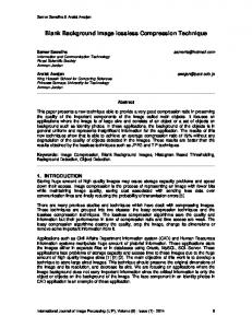
tween mindouble and maxdouble3 . This memory contains4 concatenation of one sign bit, 11 exponent bits and 52 mantissa bits. The function Int: [mindouble, maxdouble] → {0, ..., 264 − 1} is continuously growing everywhere except in 0. This function is very close to linear on every interval such as [2k , 2k+1], −1023 ≤ k ≤ 1023. A fragment of the function graph is shown in the Figure 1(a), where Int(x) is given in hexadecimal notation. The function Real(x) is opposite to Int(x), i.e. the equality Real(Int(x)) = x take place. For integer p, the Bin(p, r) is a r-bit sequence of zeros and ones of the binary representation of p (1 ≤ r ≤ 64, |p| < 2r ).

2.2 Definition of differences Assume an array b containing 64-bit integers bi , i = 1, ..., n is given. The first difference is defined as ∆1 bi = bi − bi−1 . The m-th difference is defined in a similar way as m m−1 m−1 ∆ bi = ∆ bi − ∆ bi−1 . Instead of storing the whole array b we can just store the m-th differences for b. In this case we need storage for n values: (b1 , b2 , ..., bm , ∆m bi+1 , ∆m bi+2 , ..., ∆m bn ) The sequence b can be unambiguously restored from the m-th differences. Since b elements are integers, it is restored without loss of precision. The difference between two 64-bit integers can be stored in 64 bits. In general case 65 bits would be needed, but we utilize the wrap-around feature of computer integer arithmetics. This feature can be illustrated by computation: If b1 = 263 − 1 and b2 = −(263 − 1) then b2 − b1 produces 2. Also, b1 + 2 = b2 . From above it can be concluded that a sequence b of length n can be stored as m-th differences for b , and it will occupy not more than the same memory i.e. 64n bits.

2.3 Truncating meaningless bits. We can use the fact that the difference between the array elements is small relatively to the element values. Small integer numbers have many initial zeroes (in positive numbers) or ones (in negative numbers) in their binary representation. These meaningless bits can be truncated. For instance, zeroes in 00000101 can be truncated and just 0101 is stored. Formally, truncating of bit sequences can be described as follows: Assume, s is a binary digit sequence of k elements (s1 , ..., sk ) where si ∈ {0, 1}. Then Drop(s) is defined as such substring (sl , ..., sk ) that all digits at the beginning of the original sequence are equal: s1 = s2 = . . . = sl and after that some other digit follows: sl 6= sl+1 . Normally mindouble ≈ −10309 and maxdouble ≈ 10309 are predefined compiler constants. This description can be processor-dependent; it holds for Intel, Alpha and Sparc families. The numbers can be investigated by a trivial C program. Order of bytes is, however, different: Intel and Alpha are “littleendian”, whereas Sparc is “big-endian”. This is taken into account by compression/decompression routines. 3 4

4

400199999999999a 4000000000000000 3ffe66666666666a 3ffcccccccccccd0 3ffb333333333336 3ff999999999999c 3ff8000000000002 3ff6666666666668 3ff4ccccccccccce 3ff3333333333334 3ff199999999999a 3ff0000000000000 3fee66666666666a 3fecccccccccccd0 3feb333333333336 3fe999999999999c 3fe8000000000002 3fe6666666666668 3fe4ccccccccccce 3fe3333333333334 3fe199999999999a 3fe0000000000000 3fdccccccccccccd

0

0.5

1

1.5

2

2.5

(a)

a4

c4

f c3 a3 a2

a1 t1

time t2

t3

t4

(b) Figure 1: (a) The graph of function Int(x). (b) Finding first order differences c3 and c4 .

5

Two extreme cases are defined: Drop(00 . . . 0) = Drop(0) = 0 and Drop(11 . . . 1) = Drop(1) = 1. For instance, Drop(00000101)=0101, Drop(1111111101001)=101001.

2.4 The difference compression algorithm The algorithm compresses a sequence of real numbers a to bit sequence e using differences of order m. It consists of the following steps: — The integer values are taken instead of real: bi = Int(ai ), i = 1, ..., n; — First m values are copied: ci = bi for i = 1, ..., m; — The m-th order differences are computed: ci = ∆m bi for i = m + 1, ..., n. See c3 and c4 on Figure 1(b). Further the systematic coding method is applied to c, i.e.: — Only necessary bits are selected di = Drop(Bin(ci , 64)); — The bit string length5 and the bit string itself are stored: ei = Concatenate(Bin(Length(di ), 6), di) where Concatenate is the bit string concatenation operator. — All ei are concatenated to the single bit string e = Concatenate(e1 , ..., en ). The sequence a can be restored again from e unambiguously by reverse operations6. For example (see bi in Table 2), ∆1 b2 = b2 − b1 = 00 00 00 05 3e 2d 62 39 ∆1 b3 = b3 − b2 = 00 00 00 05 3e 2d 62 3b ∆2 b3 = ∆1 b3 − ∆1 b2 = 00 00 00 00 00 00 00 02 It can be noted that the first difference requires 5 bytes (more exactly, 36 bits). The second difference requires no more than 3 bits (010). Also, 6 bits are used to encode the length. Assuming that the algorithm stores b1 , b2 and ∆2 b3 and compression ratio (64 ∗ 3)/(64 ∗ 2 + 6 + 3) ≈ 1.401 is achieved. Normally there is no smoothness in the sequence e, therefore it cannot be compressed anymore7.

3 Using fixed step extrapolation The algorithm of differences of order m can be formulated differently in terms of extrapolation of order (m−1). When this reformulation is done, just slightly different8 computations take place, and these can be seen from different point of view. We introduce the extrapolation technique here (instead of differences) in order to proceed later to varying step extrapolation algorithm in Section 4. 5

Note that there can be various approaches for length storage, for instance ei = Concatenate(di , ENDMARKER), but we found that our solution is close to optimal. This length can be coded in 6 bits because 26 = 64. 6 It can be done since result of 64-bit integer addition and subtraction is identical on all processors working with 64-bit integers. 7 Relatively small additional smoothness can be found in the sequence of Length(di ), but we ignore this for brevity. 8 Discussed in more detail in [5] .

6

The fixed step difference algorithm works well if the sequence Int(a) can be approximated by polynomials. In real applications, however, it would be better to assume that a can be approximated by polynomials9. To explore this approach traditional Lagrange extrapolation form [2] should be used. The Lagrange rule for extrapolation of order m − 1 states that for function f (x) and extrapolation points x1 , ..., xm there exist a polynomial ϕm (x) such that ϕm (xi ) = f (xi ) for i = 1, ..., m. The polynomial10 can be found as ϕm (x) = L1 (x)f1 + . . . + Lm (x)fm , where fi = f (xi ) and Li (x) =

(x − x1 ) . . . (x − xi−1 )(x − xi+1 ) . . . (x − xm ) (xi − x1 ) . . . (xi − xi−1 )(xi − xi+1 ) . . . (xi − xm )

The compression algorithm using fixed step extrapolation of order m − 1 first takes sequence of real numbers a and produces a sequence of integers c. First, m first values are copied: cj = Int(aj ) for j = 1, ..., m. After that every cj where j = m + 1, ..., n is sequentially computed as follows: 1. The m extrapolation points to the left of j are chosen: x1 = j − m, ..., xm = j − 1. 2. Correspondingly, function values are set as f1 = aj−m , ..., fm = aj−1 . 3. The predicted value ϕm (x) for x = j is computed using the Lagrange formula. 4. The extrapolation residual (difference between actual and predicted value) is stored (therefore our method is a variant of predictive coding). Since we expect that this difference is very small, the values are first converted to the integer representation and then subtracted: cj = Int(aj ) − Int(ϕm (j)) After that the necessary operations with c are performed just like in the Section 2.4.

3.1 Decompressing The original sequence a can be unambiguously restored from the compressed sequence: First, sequence of integers c is restored from the bit string e. Then first m values are copied: aj = Real(cj ) for j = 1, ..., m. After that from every cj where j = m + 1, ..., n the value aj is sequentially computed as follows: 1. The m extrapolation points to the left of j are chosen: x1 = j − m, ..., xm = j − 1. 2. Correspondingly, function values are set as f1 = aj−m , ..., fm = aj−1 . 3. The predicted value ϕm (x) for x = j is computed using the Lagrange formula. 4. The actual value is computed as sum of predicted value and the residual: aj = Real(Int(ϕm (j)) + cj ) Evaluation of ϕm (j) includes double precision arithmetics that potentially can give different results on different processors, since they use different technique to round up multiplication or division result to fit it into 64-bit space. To guarantee lossless decompression, The correlations between two and more arrays (a[1] , a[2] , a[3] , ..., a[r] ) of the same length can be taken into account. It might produce high compression ratio, specially if appears that a[k] ≈ p(t, a[1] , a[2] , a[3] , ...) and p is a polynomial. These correlations can be revealed automatically, however this is rather time consuming. 10 Note that the term xi − xi is always skipped in the divider. If x1 = j − 3, x2 = j − 2, x3 = j − 1 then ϕ3 (j) = f (j − 3) − 3f (j − 2) + 3f (j − 1). 9

7

it should be made on the same processor family as compression. Otherwise an error in the last bit might appear, accumulate and lead to losing numerical accuracy11 . The algorithm is fast since the coefficients for Lagrange formula are computed efficiently and only once (see [5] for details)

4 Varying step extrapolation algorithm The previous algorithms assumed that the sequence a can be approximated by polynomials with fixed steps between extrapolation points. However in practice, simulations use adaptive ODE solvers and produce state variable values for varying, non-equidistant time steps. Therefore we should consider smooth functions with values taken with varying steps, and adapt the compression algorithm for such application data. Assume that a function f : [tmin , tmax ] → R is evaluated during the simulation. Finite number (n) of function values is produced by the solver for time steps (t1 , ..., tn ) (where tmin = t1 , tmax = tn , ti < ti+1 ) and these are stored in the sequence, a so that ai = f (ti ). The sequence t is used for compression and decompression of a. The sequence t itself should be compressed by the fixed step difference algorithm. The compression algorithm using varying step extrapolation of order m − 1 first takes the sequence of real numbers a and t and produces a sequence of integers c. First, m first values are copied: cj = Int(aj ) for j = 1, ..., m. After that every cj where j = m + 1, ..., n is sequentially computed as follows: 1. The m extrapolation points to the left of j are chosen: x1 = tj−m , ..., xm = tj−1 . 2. Correspondingly, function values are set as f1 = aj−m , ..., fm = aj−1 . 3. The predicted value ϕm (x) for x = tj is computed using the Lagrange formula. 4. The residual (difference between actual and predicted value) is stored. Since we expect that this difference is very small, the values are first converted to the integer representation and then subtracted: cj = Int(aj ) − Int(ϕm (tj )) After that the necessary operations with c are performed just like in the Section 2.4. The original sequence a can be unambiguously restored from the compressed sequence under conditions described in the Section 3.1.

5 Experiments In this chapter we describe the experimental application of both our algorithms — higher order differences (suitable for fixed steps) (orders 2, 4, 6, 8, 10) and varying step extrapolation (of orders 1, 3, 5, 7, 9). The compression ratios are compared with two wavelet algorithms (Section 5.1). There were two major tests: artificially designed test sequences and output from high-precision numerical simulation of mechanical model using ODE solver. 11

Our experiments with Sparc and Alpha processor families show that difference is never larger than 2-3 last bits when extrapolation of 3rd order is used and n = 100.

8

5.1 Experiments with wavelet-based algorithms A widely used family of algorithms for numerical data compression are wavelet transforms. Without going into details about wavelet theory and taxonomy of transforms we just describe two transforms we experimented with. Assuming that a sequence has some correlation between neighbor elements, wavelet transform computes an “average” value s and “difference value” d. For arbitrary integer q > 0 the transform compresses a sequence a0 , ..., aQ , where Q = 2q+1 − 1, by running through levels r = q, q −1, ..., 0. On the level r the sequence considered is a0 , ..., aR , where R = 2r+1 − 1. Furthermore there are certain rules defining how to compute the sequence for level r − 1. The simplest wavelet transform, Haar wavelet [3] computes on level p by formulae si = (a2i + a2i+1 )/2,

di = a2i+1 − a2i

i = 0, ..., 2r − 1

The number of bits needed for di is relatively small; lossy compression algorithm using wavelets might ignore it; the lossless algorithm stores them. The elements si become ai on the next level of transform. The sequence a can be recovered by a2i = si − di /2, a2i+1 = si + di /2. This algorithm is specially successful for sequences which change very slowly and close to a polynomial function. Mainly wavelet algorithms are used for lossy compression. There are, however, modification, called TT-transform [4], used for lossless compression: si = b(a2i + a2i+1 )/2c, di = a2i − a2i+1 + pi , where pi is defined by pi = b(3si−2 − 22si−1 + 22si+1 − 3si+2 + 32)/64c, and sequence can be restored by a2i = si + b(di − pi + 1)/2c, a2i+1 = si − b(di − pi )/2c Both Haar and TT transforms were applied to compression and decompression. Just like in Section 2.4 six bits were always used to encode the length of the bit strings. The experiments show that compression ratio for lossless compression is insufficient.

5.2 Artificially designed test sequences. The test sequences for testing the algorithms were designed. These sequences contain 64-bit double precision numbers. We took into consideration that the sequence for the test cases should be rather smooth as a whole, but it should also contain small local non-smooth variations. The size of the sequence N is chosen as 28 or 216 (see Table 3). The longer sequence has smaller difference between adjacent elements and therefore is compressed better. The sequence a with fixed time steps is defined as ai = F (i/N) where i = 1 . . . N and F (x) = 0.2 + 0.7x − 0.5x2 + 0.007 cos(100x) + 0.00007 cos(10000x) + 0.1 sin(10x) The time step is constant 1, i.e. ti = i. The table shows that sequences with fixed time step can be compressed equally well by both our algorithms (see repetitions in columns under ”fixed”)). The best ratio achieved is 3.68. For testing of a sequence with varying time step we use ti = ti−1 + imod4 + 1 and ai = F (2−16 ti /2.5) where i and F are as above. Here time steps vary from 1 to 4. Therefore the algorithm using varying step extrapolation shows better result than the algorithm using differences (3.73 versus 1.3). 9

Ratio Time step: Number of values: m=2 Differences 4 of order 6 m 8 (Section 2.4) 10 Varying m=1 step m-th 3 order 5 extrapolation 7 (Section 4) 9 Wavelet TT Haar

fixed 28 216 1.58 1.64 1.81 1.9 2.12 2.27 2.52 2.8 3.13 3.68 1.58 1.64 1.8 1.9 2.11 2.27 2.51 2.8 3.11 3.68 1.7 1.86 1.39 1.47

varying 28 216 1.45 1.53 1.43 1.51 1.33 1.42 1.27 1.35 1.23 1.3 1.58 1.65 1.81 1.91 2.12 2.29 2.54 2.83 3.16 3.73 1.23 1.67 1.19 1.4

Table 3: Compression ratios for various data sequences and various algorithms.

5.3 Application to simulation results The compression algorithms were applied to the output from a numerical solver of ordinary differential equations, which serves as a component in our software for dynamic simulation of bearing [1]. The program produces some quantities for every time step and writes them to the output file for analysis and further simulation. Every quantity (position, force etc.) changes very slowly from one step to another. Extreme accuracy and lossless compression is necessary, since a relative error of order 10−10 can substantially change the simulation results. To chose a particular algorithm and its order the compression routines estimate achievable compression ratio by subsampling, trying different algorithms and choose the best one. The 2837 arrays from a single simulation were analyzed. Compression ratio varies between 2.5 and 10. The algorithms were automatically chosen as follows: — difference, first order - 20% of all arrays12 , second order - 3%, 3rd order - less than 1%. — varying step extrapolation, first order -10 %, second order - 17%, third order - 51%. If the 4th order extrapolation is suggested, it takes 30%, but compression ratio is almost the same as in the 3rd order extrapolation.

5.4 Lossy compression There were four different applications of data saved by the compression algorithm: — simulation can be restarted from any time step; 12

These arrays are not smooth. It took 40 bits per 64-bit number to compress them. Compression ratio was

1.6.

10

— simulation results are used in another computation; — intermediate simulation results are sent between nodes in parallel simulation; — simulation results are visualized in form of 2D function graphs and 3D model animations. Only the last application allows using lossy compression. Other applications require lossless one. The lossy compression is an extension of the basic algorithm. It can be parameterized in order to adjust the trade-off between the precision and the compression ratio. The lossy compression can be achieved by cutting away some c bits at the end of the bit string representation. To compensate for the error one exact value is followed by some p lossy compressed values. The user would be interested to choose the pair (c,p) for given sequence a in such a way that during decompression the absolute and relative error does not exceed εabs and εrel correspondingly. There is a straightforward way to do that, but it requires some extra computations during compression. First we use an interval [amin , amax ], where amin = min(ai −εabs , ai −εrel kai k), amax = i i i i max(ai + εabs , ai + εrel kai k). After that interval arithmetics is used in order to obtain [dmin , dmax ]. Then di is easily i i chosen from this interval such way that it occupies the minimal possible number of bits.

6 Conclusion A lossless algorithm for floating-point data compression has been developed. It has similarities to image compression, since it works on bit level. It resembles wavelet compression since it uses floating-point computations for compression and decompression. The algorithm works best if the data are values of a function in some points, and this function is close to a polynomial. The algorithm uses subtraction of one 64-bit integer representation of floating-point value from another (Int(aj )−Int(ϕm (tj ))). If the difference would be computed between floating-point representations (aj − ϕm (tj )) there would be no win in data storage. The algorithm is implemented as a C++ class and linked to an industrial-level application. The measurements show high compression ratio (in comparison with traditional tools) as well as high speed[5]. In the future we are going to test and measure the algorithm with the data samples from other applications.

Acknowledgments Professor Robert Forchheimer (ISY, Link¨oping University) contributed many suggestions regarding the discussed algorithms.

11

References [1] D. Fritzson, P. Fritzson, P. Nordling, T. Persson. Rolling Bearing Simulation on MIMD Computers. Int. Journal of Supercomp. Appl. and High Performance Computing, 11(4), 1997. [2] R˚ade, L., Westergren, B., Beta - Mathematics Handbook, Studentlitteratur and Chartwell-Bratt, 1988, p.336. [3] A. Certain, J. Popovic, T. DeRose, T. Duchamp, D. H. Salesin, W. Stuetzle. Interactive multiresolution surface viewing. Proceedings of SIGGRAPH 96, in Computer Graphics Proceedings, Annual Conference Series, 91-98, August 1996, http://www.cs.washington.edu/research/projects/grail2/www/pub/abstracts.html #InterMultSurfView [4] M. J. Gormish, E. L. Schwartz, A. Keith, M. Boliek, A. Zandi, Lossless and nearly lossless compression for high quality images Proc. of IS&T/SPIE’s 9th Annual Symposium, Vol. 3025, San Jose, CA, February 1997. [5] Vadim Engelson, Dag Fritzson, Peter Fritzson. On Delta-compression Algorithm for Numerical Data from ODE-based Applications in Scientific Computing Technical reportPELAB, Link¨oping University, 1999.

12

Version: January 13, 2000

13