Lossless Data Embedding with File Size Preservation. Jessica Fridrich. ∗. ,
Miroslav Goljan, Qing Chen, and Vivek Pathak. Department of Electrical and ...
Lossless Data Embedding with File Size Preservation Jessica Fridrich∗, Miroslav Goljan, Qing Chen, and Vivek Pathak Department of Electrical and Computer Engineering SUNY Binghamton, Binghamton, NY 13902-6000, USA ABSTRACT In lossless watermarking, it is possible to completely remove the embedding distortion from the watermarked image and recover an exact copy of the original unwatermarked image. Lossless watermarks found applications in fragile authentication, integrity protection, and metadata embedding. It is especially important for medical and military images. Frequently, lossless embedding disproportionably increases the file size for image formats that contain lossless compression (RLE BMP, GIF, JPEG, PNG, etc…). This partially negates the advantage of embedding information as opposed to appending it. In this paper, we introduce lossless watermarking techniques that preserve the file size. The formats addressed are RLE encoded bitmaps and sequentially encoded JPEG images. The lossless embedding for the RLE BMP format is designed in such a manner to guarantee that the message extraction and original image reconstruction is insensitive to different RLE encoders, image palette reshuffling, as well as to removing or adding duplicate palette colors. The performance of both methods is demonstrated on test images by showing the capacity, distortion, and embedding rate. The proposed methods are the first examples of lossless embedding methods that preserve the file size for image formats that use lossless compression. Keywords: Embedding, lossless, erasable, invertible, removable, distortion, file size preservation, RLE, JPEG
1. INTRODUCTION Lossless embedding is a term for a class of data hiding techniques that are capable of restoring the embedded image to its original state without accessing any side information. One can say that the embedding distortion can be erased or removed from the embedded image. This is why some researchers refer to this type of embedding as erasable, removable, invertible, or distortion-free. The idea of lossless embedding was for the first time proposed by Honsinger1 in 1999. This technique, originally designed for lossless authentication, suffered from visible distortion (for some images) and limited capacity. Fridrich et al.2 introduced a general methodology for lossless embedding in digital images that is based on lossless compression of image features. In this method, one first selects a subset X of image features that is losslessly compressible and that can be randomized without causing visible degradation to the image. The lossless embedding proceeds by compressing X to C(X) and replacing X with C(X) & {m j }Lj=1 , where mj are the message bits and ‘&’ denotes concatenation. This way, one can losslessly embed up to |X|–|C(X)| bits. This embedding paradigm is very general and many schemes can be designed by selecting different image features2,3. Alternative approaches to lossless embedding were later proposed by Macq4, Tian5, and Kalker6. Researchers have focused on different aspects of lossless embedding schemes. Increasing the lossless embedding capacity has recently been the principle motivation3,5,6. Celik3 described a lossless authentication method with localization. Kalker et al.7 proposed an approach that minimizes distortion per embedded bit. The first lossless embedding scheme for audio signals has been described by Kalker6.
∗
[email protected]; phone: 1 607 777-2577; fax: 1607 777-4464; http://www.ws.binghamton.edu/fridrich; SUNY Binghamton; Watson School of Engineering, Dept. of Electrical and Computer Engineering, Binghamton, NY USA 13902-6000
So far, little attention has been paid to the increase of the file size introduced by lossless embedding. In lossless embedding schemes designed for image formats that use some form of lossless compression, the increase in the file size could be many times larger than the actual number of embedded bits L. This inefficiency partially outweighs the advantage of embedding the data as opposed to appending it to the cover image. In fact, the sponsors of this research∗ have expressed the need for lossless embedding schemes that preserve the file size. The act of lossless embedding of a random message stream increases the entropy E(I) of the cover image I to E(Y)=E(I)+L, where Y is the embedded image. Fortunately, any specific lossless compression algorithm does not compress Y to the ideal E(Y) bits but to |C(Y)| bits, where |C(Y)|>E(Y) and C(Y) is the compressed embedded image. Consequently, one can theoretically at most |C(Y)|–E(Y) bits losslessly and still preserve the file size+. To design such a scheme, however, one will likely have to tailor it to the specific compression scheme as well as the image format. For example, if the cover image is an RGB encoded BMP file, the embedding does not increase its file size because the RGB BMP format does not incorporate any compression. However, the run length encoded (RLE) BMP, GIF, and JPEG contain lossless compression8 (runlength, LZ77, and Huffman, respectively). Thus, the embedded file has a different, usually larger, size than the original. This paper is the first step to developing lossless embedding techniques that preserve the file size. We have chosen two of the most common formats – the RLE encoded BMP image format and the ubiquitous JPEG format. In the next section, we describe the RLE compression algorithm and then, in Section 3, the RS lossless embedding scheme with file size preservation is introduced. Experimental results are presented in Section 4. In Section 5, we describe the relevant details of the JPEG format and the lossless file-size preserving technique. The algorithm performance is discussed in Section 6. Conclusions and future research are included in Section 7.
2. RLE COMPRESSION Run length encoding (RLE) is a simple lossless compression that assigns short codes to long runs of identical symbols. It is used in the BMP format for images with up to 256 colors. The RLE format decoding rules are simple: nB 00 01 02xy 0 n A1…An (0)
decode as byte B repeated n-times, n≥1, EOL; end of row, EOB; end of bitmap, Delta; move x pixels to the right and y pixels down, n≥3, decode as A1…An , zero is padded when n is odd.
The last decoding rule is called the “absolute mode”. An important observation is that although the decoded image is always unique, the encoding can be done in many different ways. For example, some RLE implementations never use the code “nB” for n=1 but use the absolute mode instead. Therefore, different RLE encoders may generate files with slightly different sizes.
3. LOSSLESS EMBEDDING WITH FILE SIZE PRESERVATION FOR RLE BMPs 3.1 Problem statement Because there exist many different RLE encoders, the embedding scheme must also guarantee that the message and the original image can be extracted from the embedded and encoded image independently of the RLE encoder.
∗
The Air Force Office of Scientific Research and the Air Force Research Laboratory in Rome, NY.
+
In practice, however, we are not likely to achieve this capacity because the embedded image must be perceptually equivalent to the original image.
We have decided to use the RS lossless data embedding method2 as our starting point for the design of a lossless filesize preserving method. This method seemed to be the most amenable to modifications that would enable us such construction. Lossless embedding with file size preservation for RLE compressed images (LE4RLE) should satisfy the following requirements: (R1) The file size of the original and the embedded images must be equal after RLE compression using virtually any RLE compressor. (R2) The original image can be retrieved from the embedded image exactly. (R3) Any image processing that does not modify image content (image renaming, palette reordering, removing or introducing duplicate entries in the palette, image lossless compression and/or decompression of any kind) must not lead to message extraction failure. (R4) The message and the original image can be retrieved from both RLE compressed and decompressed images. (R5) Embedded images should be perceptually equivalent to their originals, keeping the embedding distortion as low as possible. 3.2 Defining concepts In this section, we briefly introduce the concepts needed for the description of the RS embedding method2 and its LE4RLE modification that preserves file size (in Section 3.4). First, all palette colors are divided into disjoint (unordered) pairs {ci, cj} of perceptually similar colors (some colors may be paired to themselves). The set of all color pairs is denoted as P. Furthermore, for each color ci , we define its flipped color as ci = cj, where {ci, cj} is a color pair from P. Next, we extend the flipping operation to a group of k pixels with colors (c1, c2, …, ck) and a binary mask M∈{0,1}k : G M = (c'1 , c'2 ,..., c'k ) , where G = (c1, c2, …, ck) and c M i = 1 ci ' = i , i = 1, …, k . ci M i = 0 The mask M can be the same for all groups (as it is the case in the original RS embedding) or be individually defined for each group (in this paper). We further define the discrimination function f(G) k −1
f (G ) = f (c1 , c2 ,..., ck ) =
∑ d (c , c i
i +1 )
,
(1)
i =1
where d is the distance between two colors. The selection of color pairs and the distance d is detailed in Section 3.5. Finally, we describe a function that assigns one bit b(G) to each group G: 0, f (G ) − f (G ) > T (2) b(G ) = 1, f (G ) − f (G ) < −T undefined, f (G ) − f (G ) ≤ T . The threshold T can be used to achieve different capacity-distortion rate (see Section 4). Note that for natural images the flipped group G will be “noisier” than G and thus Prob{f( G )>f(G)}>1/2. Consequently, b(G) will have more 0’s than 1’s. Because G = H ⇔ G = H , we have b(G ) = 1 − b(G ) , whenever b(G) is defined. Also, b(G) is defined if and only if b(G ) is defined.
3.3 RS lossless embedding Following the original method, the RS lossless embedding starts by dividing the original image X into disjoint groups of the same size and shape (e.g., 2×2 blocks). Let Gi, i=1, 2,…, N be all the groups for which bi = b(Gi) is defined. The RS algorithm flips some of the groups Gi to Gi′ so that their associated bits bi′ = b(Gi′) encode the message and the (compressed) original bits C ({bi }iN=1 ) & {m j }Lj=1 , where C({bi}) is the losslessly compressed∗ bit-stream {bi} needed for reconstruction of the original image. Note that because the bit-stream {bi} contains more 0’s than 1’s, it will be losslessly compressible. As a result, this method can embed up to N–|C({bi})| message bits mj. At the decoder, the compressed bit-stream C({bi}) and the message bits {mj} are extracted. Then, the groups Gi′ are flipped as needed to match their associated bits bi with the extracted and decompressed bit-stream {bi} thus obtaining an exact copy of the original image. Next, we explain how this scheme can be modified to guarantee file size preservation for RLE encoded BMP images. 3.4 RS lossless embedding with file size preservation In the RLE BMP format, the image data X is represented by indices xi to the image palette, which can have up to 256 entries. Let c(xi) denote the color of the pixel xi. During embedding, each pixel xi can either stay unmodified or be changed to xi , where xi is the index to the color c( xi ) . We start with a simple observation that the size of the RLE compressed image will not be changed by embedding if the length of all runs (along image rows) is not changed. This means that any sequence of pixels ‘yxx…xz’ can be changed to ‘yww…wz’ by replacing x with w, w≠y and w≠z. Given the image X ={xi}, i=1, 2,…, Np, represented as a row vector (pixels arranged by rows), we define the invariant image R={ri} as ri = min{xi , xi } , i=1, 2,…, Np . Thus, the image R does not distinguish between the colors in the pair {c( xi ), c( xi )} ∈ P. When scanning a row of pixels in R, transform this image using the RLE code “nB” only, whenever the index B is repeated n times, and as “00” for End of Line. The sequence of numbers n determines the length of row segments that the embedding algorithm must leave unmodified or modify simultaneously to nB . Because each segment will carry the same amount of hidden information regardless of its length, to keep the distortion low, it is better to limit the length of each segment to a small number. In this paper, we use segments consisting of exactly one pixel. The set of all pixels that belong to such segments of length 1 will be denoted as Q xi∈Q ⇔ (ri ≠ ri–1 and ri ≠ ri+1). If the embedding algorithm flips only the pixels in Q, the file size of the embedded image will be preserved under any RLE encoder. Thus, the lossless method with file size preservation proceeds in the same way as the original RS method with one difference – the mask M for each group G is determined by pixels from Q. This mask will reflect which pixels can be modified and which cannot. To obtain the individual masks, we define a binary matrix E=(ei), of the same size as the image, that captures which pixels may (1) and must not (0) be modified 1 xi ∈ Q ei = 0 xi ∉ Q.
∗
In RS method2, adaptive arithmetic coding was used to compress the bit-stream b(Gi).
Each group of k pixels ( xi1 , xi2 ,..., xik ) with colors G = (c( xi1 ),K, c ( xik )) will have its own embedding mask M M = (ei1 , ei2 ,..., eik ) . Thus, G M = (c1 ' , c2 ' ,.., ck ' ) , where
c( xi ) xi ∈ Q j j c j '= c( xi j ) xi j ∉ Q . Note that the embedding mask can be uniquely determined from both the original and embedded images.
Now, let us summarize all steps of lossless embedding with file size preservation. Encoder 1. 2. 3. 4. 5. 6.
Determine pairs of close colors P (see Section 3.5) Calculate the set Q of modifiable pixels. Divide the image into disjoint groups G. Calculate bi = b(Gi) for all groups of pixels whenever they are defined. Use a pseudo-random order for index i of Gi. Start compressing the bit sequence {bi} to C{bi}. Stop the compression at bk as soon as the inequality k ≥ l + L + length(C{bi} ik=1 ) is satisfied (l is the number of bits that encodes message length). Form the composite message Message_length & Message_bits & C{bi} spanning l, L, and V bits. For each i, if (bi ≠ i-th bit of C{bi}&{mj}) then flip Gi to Gi .
Decoder 1.–2. The same as in Encoder. 3. Divide the image into disjoint groups G. Calculate b′i = b(Gi) for all groups of pixels whenever they are defined. Use the same pseudo-random order for index i of Gi as during embedding. 4. Read b1′ b2′… bl′ and message bits b′l+1 b′l+2… b′l+L. 5. Set j=1. Decompress the segment b′l+L+1 … b′l+L+j and denote the length of the decompressed segment V. 6. If V < l+L+j then Go to 5, else Stop. The decompressed bits are b1b2 …bl+L+V. 7. For i =1, …, V, if (bi ≠ b′l+L+i), flip Gi to Gi . Because both the encoder and decoder start from the image decompressed to the spatial domain, the method is insensitive to differences between RLE encoders. Also, presorting the palette to a fixed order (e.g., alphabetically) before determining color pairs P will make the system work after palette reshuffling. The problem of removing or adding duplicate palette entries can be addressed by unifying duplicate entries in the palette to the lowest one from all duplicate indices before embedding and returning the occurrences of the duplicate colors after embedding. In particular, let c1, c2, …, ck are different palette entries corresponding to one RGB color, c1 < c2 < … < ck. Before embedding, we modify all pixels with colors c2, …, ck to c1. After embedding, the pixels with colors c1 are changed back to cj if they were equal to cj in the original image, for all j = 2, …, k. The first step guarantees that it will not matter whether or not the duplicate entries are removed and the last step guarantees that the file size will not decrease during data insertion. 3.5 Color pairing and distance d Let D = {dij}, i, j =1, …, n, n ≤ 256, be the matrix of distances between colors i and j after presorting the colors that appear in the image. These distances can be measured in any color space, such as RGB, YUV, or CIELAB. After subjectively evaluating results of experiments with different spaces, we selected the square of the weighted Euclidean RGB distance d = wr 2 (ri − r j ) 2 + wg 2 ( g i − g j ) 2 + wb 2 (bi − b j ) 2 ,
where wr = 0.35, wg = 0.4, and wb = 0.25, and ri, rj, gi, gj, bi, and bj are integers in the range from 0 to 255.
Once an appropriate distance measure d in the RGB color space is established, one can attempt to determine the color pairing P that minimizes the distortion with a lower bound on the capacity or maximize the capacity with an upper bound on the distortion. Such problems can be formulated as an optimal incomplete matching problem10 in a weighted graph with three weights at each edge and with one constraint. Since the optimal matching can be incomplete, some colors can be paired to themselves. There is no known algorithm for solving this task efficiently in a polynomial time. We skip the details here due to a limited space. Below, we describe a heuristic algorithm that strives to provide good capacity-distortion trade off. 3.5.1 Top-down color matching algorithm In our previous work2, we have introduced the color matching algorithm called “Top-down”. In this paper, we use an improved version of this approach that gives higher embedding capacity with lower distortion. The top-down matching algorithm starts with the most isolated color and finds its closest neighbor among all remaining colors. If the distance between these two colors is below a fixed threshold t, both colors are removed from the set of all colors and declared as a “close pair”. If the distance is larger than the threshold, the most isolated color is paired with itself and removed. This step is repeated until all colors are paired. The parameter t regulates the trade-off between image distortion and lossless capacity. Next, we describe a modification of this algorithm that has achieved better results in our experiments. 3.5.2 Improved top-down color matching algorithm Instead of the most isolated color, this algorithm finds colors with the least number of colors within the distance t. Among them, the pair with its distance closest to t is chosen and removed from the set. This step is repeated until no such pair can be found. The pseudo-code for this algorithm follows. k = 1; 0, when d ij = 0 or d ij > t bij = 1, otherwise (0 < dij ≤ t ) si =
∑b
ij
, ni = min {d ij } ; for all i j , 0 < d ij ≤ t
j
Repeat
m = min{si } ; si > 0
a = arg max{ni } ; b = arg min{d aj } ; i, si = m
j , baj =1
Set (a, b) as the k-th pair, k=k+1 ; sa = 0 ; sb = 0 ; For all si > 0 set si = si – bia – bib ; bia = 0 ; bib = 0 ; i = 1, …, n ; until (si = 0 for all i)
4. EXPERIMENTAL RESULTS In our experiments, we have used “column” groups G consisting of 4×1 pixels. Because the RLE compression proceeds by rows, such groups provide better capacity than groups of 2×2 or 1×4 pixels. In the original RS method, the threshold T in (2) was set to 0. For color palette images, however, it is advantageous to make T proportional to t to improve the capacity without increasing the embedding distortion. A linear dependence T = 0.7t gave us good results for a wide range 0 < t ≤ 50. We note that this relation depends on our choice of the distance measure d.
For brevity, we demonstrate the performance of the proposed method for only 5 test images. Four images were 640×480 true color images (Lenna was 512×512) converted to 256 colors using PaintShop Pro 4.12 with the optimized palette and nearest color options. For all test images, we calculated the capacity (in bits per pixel or bpp), distortion (PSNR), and rate in bits per unit distortion measured in the L1 norm. Table 1 shows the results for the LE4RLE method that preserves the file size and the original RS method. In the last column, the table also shows the file size increase ∆ (in bytes) produced by the original RS method when embedding the maximal length message (the compression was done in the same version of PaintShop Pro). This file size increase bears almost no relationship to the message size (surprisingly) and is mostly influenced by the image content and the efficiency of the RLE compression. The file size increase ∆ may become very large if the act of embedding makes the image significantly less compressible using RLE (for Image No. 4, ∆ is more than 20 times larger than the message length). Of course, the new LE4RLE method did not lead to any file size increase. Inspecting the rate in Table 1, we can see that the new method achieves slightly better rate than the original RS method. The absolute capacity decreases by about 20% but, but this is fairly insignificant because the capacity can be adjusted with the parameter t that controls the distortion-capacity trade off (Table 2). Overall, the capacity of the new method is large enough for applications, such as authentication or annotation embedding – the main applications for which the concept of lossless data embedding was originally introduced. Image Im_1 Im_2 Im_3 Im_4 Lenna
LE4RLE bpp (%) PSNR
3.08 1.90 4.63 4.21 6.48
33.3 33.4 34.7 34.6 30.3
RS Rate
bpp (%)
PSNR
Rate
.0076 .0050 .0127 .0125 .0148
4.28 1.89 5.51 5.41 7.70
31.4 32.0 33.3 32.1 27.3
.0065 .0032 .0108 .0103 .0088
∆
Image
9172 7634 2286 33440 3186
Im_1 Im_2 Im_3 Im_4 Lenna
Table 1. Capacity, distortion, and rate for 5 test images for LE4RLE and the original RS method, t = 20. ∆ (Byte) is the difference in file size in the original RS embedding.
Im_1
Im_2
Im_3
Capacity (% of bpp) t=10 t=30 t=40 1.44 3.98 4.01 0.81 2.18 4.12 1.68 6.05 6.91 1.82 6.25 7.52 3.97 8.92 10.58
t=10 37.02 38.20 39.30 40.26 33.14
PSNR (dB) t=30 t=40 31.35 29.50 33.15 31.56 31.25 30.01 31.97 30.53 31.16 29.04
Table 2. Capacity and distortion as functions of the parameter t for several test images.
Im_4
Lenna
5. LOSSLESS EMBEDDING WITH FILE SIZE PRESERVATION FOR THE JPEG FORMAT The JPEG format9 is the most popular image format in current use. This is because it offers a convenient trade off between the file size and the perceptual quality of the encoded image. Our previously developed lossless embedding schemes2 for JPEG do not preserve the JPEG file size and in some cases the file size increase can be quite disproportional to the embedded message size. This partially negates the advantages of embedding data rather than appending. In this section, we address this issue and describe a lossless embedding technique for sequentially encoded JPEG images that preserves their file size (within a few bytes). The JPEG encoder consists of three fundamental components (see Fig. 1): Forward Discrete Cosine Transform (FDCT), a scalar quantizer, and an entropy-encoder. After the DCT is applied to an 8×8 block of pixels transforming the block from spatial domain to the frequency domain, DCT coefficients are quantized using the quantization table. The quantized coefficients are arranged in a zigzag order and pre-compressed using the Differential Pulse Code Modulation (DPCM) on DC coefficients and RLE on AC coefficients. Finally, the symbol string is Huffman-coded to obtain the final compressed bit-stream. After pre-pending the header, the final JPEG file is obtained.
Our lossless embedding scheme with file size preservation works with the Huffman-decompressed stream of intermediate symbols. This bit-stream is modified in a careful manner to make sure that the final file size after Huffman compression stays the same within a few bytes. To understand the embedding principles, we need to describe the lossless part of JPEG compression in more detail. Message
8x8 blocks
FDCT Source Image Data
Quantizer
Entropy Encoder
Table specific ations
Table specific ations
JPEG file
Compressed Image Data
Fig. 1. Lossless embedding in JPEG files.
5.1 The JPEG entropy coder The entropy coder consists of two steps: (1) DPCM encoding of the DC term and runlength encoding of the AC coefficients into a sequence of intermediate symbols and (2) Huffman coding. The purpose of the DPCM is to decorrelate the DC term because DC coefficients from neighboring blocks still exhibit significant local correlations. The AC coefficients, on the other hand, contain long runs of zeros due to the quantization. Thus, AC coefficients are conveniently encoded using the runlength encoding. The DPCM coding of DC coefficients and the runlength coding of AC coefficients produce a sequence of intermediate symbols, which is finally entropy coded (Huffman) to a data stream in which the symbols no longer have externally identifiable boundaries. Our embedding technique works with the sequence of intermediate symbols. We ignore the DC coefficients because their modifications usually lead to visible artifacts. To explain how we modify the runlength encoded AC coefficients, we need to describe the runlength coding algorithm in more detail. 5.2 Run length encoding of AC coefficients Run length encoding (RLE) is a simple lossless compression that assigns short codes to long runs of identical symbols. As mentioned above, majority of AC coefficients in each block are usually zeros. To efficiently utilize this fact, the AC coefficients are coded in a special RLE format as pairs of intermediate symbols (S1, S2). The codeword S1 represents both the number of zeros before the next nonzero DCT coefficient and the category (number of bits required to represent its amplitude). The S2 symbol defines the amplitude and sign of the nonzero coefficient. The symbol S1, S1=(Run/Category), is a composite 8-bit value of the form S1 = binary ’RRRRCCCC’. The 4 least significant bits, ’CCCC’, define a category for the amplitude of the next non-zero coefficient in the block. The 4 most significant bits, ’RRRR’, give the position of the coefficient in the block relative to the previous non-zero coefficient (i.e., the runlength of zero coefficients between non-zero coefficients): • • •
Run (RRRR): the length of the consecutive zero-valued AC coefficients preceding the next nonzero AC coefficient, 0≤Run≤15. Category (CCCC): the number of bits needed to represent the amplitude of the next nonzero AC coefficient, 0≤Category≤15. S2 (amplitude): S2 represents the amplitude of the next nonzero AC coefficient by a signed integer.
Once the quantized coefficient data from each 8×8 block is represented in the intermediate symbol sequence described above, variable-length codes are assigned. Each S1 (Run/Category) is encoded with a variable-length code (VLC) from a Huffman table. Each S2 (amplitude) is encoded with a “variable-length integer” (VLI) code, which is an index into the amplitude value field whose length in bits is given in the second column of Table 3.
Both VLCs (S1) and VLIs (S2) are codes with variable lengths, but VLIs are not Huffman coded. They are appended to the Huffman coded S1 to form the final JPEG bit-stream. So, we can change a particular VLI as long as the modified value is from the same category (has the same length) without changing the JPEG file size. Consequently, if all the embedding changes have this property, the JPEG file size will be preserved.
Amplitude value field Category AC size 0 0 N/A –1, 1 1 1 –3, –2, 2, 3 2 2 –7,…,–4, 4,…, 7 3 3 –15,…,–8, 8,…, 15 4 4 –31,…, –16, 16,…, 31 5 5 –63,…,–32, 32,…, 63 6 6 –127,…, –64, 64,…,127 7 7 –255,…,–128, 128,…, 255 8 8 –511,…,–256, 256,…, 511 9 9 –1023,…,–512, 512,…,1023 10 A –2047,…,–1024, 1024,…, 2047 11 B –4095,…,–2048, 2048, …, 4095 12 C –8191,…,–4096, 4096,…, 8191 13 D –16383,…,–8192, 8192, 16383 14 E –32767,…,–16384, 16384, 32767 15 N/A Table 3. Runlength coding category and amplitude of AC coefficients.
5.3 Lossless embedding with file size preservation We build our lossless file size preserving method around the lossless embedding scheme for JPEGs2. As explained in the previous paragraph, in order to preserve the file size, a given DCT coefficient d from category C can only be changed to another coefficient d ’ from the same category C. To minimize the embedding distortion, we want this change to be as small as possible. Also, because changes to DC coefficients usually introduce visible distortion, we confine the embedding modifications to AC coefficients, only. Considering the requirements above, we further limit the embedding changes to the same category, swapping values of AC DCT coefficients within the following pairs: (–2,–3), (2,3) from category 2, (–7,–6), (–5,–4), (4,5), (6,7) from category 3, etc. During embedding, one value from the pair may be changed to the other value from the same pair. The value pairs are called embedding pairs. If we assign parity 0 to all even valued coefficients and parity 1 to odd valued coefficients, then the parities of the DCT coefficients that participate in embedding pairs in the original JPEG file is a binary sequence T that is losslessly compressible. This is because in natural images the distribution of DCT coefficients is generalized Gaussian centered at 0 and thus the sequence T contains more 0’s in T than 1’s. The rest of the embedding follows the RS method for JPEGs2. We first losslessly compress the sequence T, obtaining the compressed bit-stream C(T), |C(T)|