Lossless quantum data compression and variable-length coding

Lossless quantum data compression and variable-length coding Kim Bostr¨om and Timo Felbinger

arXiv:quant-ph/0105026v2 1 Mar 2002

(February 1, 2008) In order to compress quantum messages without loss of information it is necessary to allow the length of the encoded messages to vary. We develop a general framework for variable-length quantum messages in close analogy to the classical case and show that lossless compression is only possible if the message to be compressed is known to the sender. The lossless compression of an ensemble of messages is bounded from below by its von-Neumann entropy. We show that it is possible to reduce the number of qbits passing through a quantum channel even below the von-Neumann entropy by adding a classical side-channel. We give an explicit communication protocol that realizes lossless and instantaneous quantum data compression and apply it to a simple example. This protocol can be used for both online quantum communication and storage of quantum data.

Westmoreland [8]. We define a measure of information quantifying the effort of communication. Compression then means reducing this effort. We argue that prefix codes are practically not very useful for quantum coding and suggest a different method involving an additional classical side-channel. With the help of this channel, certain problems of instantaneous quantum communication can be avoided and, moreover, the quantum channel can be used with higher efficiency. At last, we present a communication protocol that enables lossless and instantaneous quantum data compression and we demonstrate its efficiency by an explicit example. Let us start with reviewing the fundamental notion of a code 1 .

I. INTRODUCTION

Any physical system can be considered as a carrier of information because the state of that system could in principle have been intentionally manipulated to represent a message. The state of a system composed from distinguishable subsystems forms a message of a certain length, where each subsystem represents one letter. In quantum information theory, the systems are quantum and the system states represent quantum messages. A message is compressed if it is mapped to a shorter message and if this map is reversible, then no information has been lost. Schumacher was the first to present a method for quantum data compression [1]. It is based on the concept of encoding only a typical subspace spanned by the typical sequences emitted by a memoryless source. Since then there have been further investigations [2–8], but all considered compression methods are only faithful in the limit of large block lengths. Now we ask: Is it possible to compress quantum messages without any loss of information? To answer this question some basic concepts of quantum information theory have to be revisited. In particular, the requirement of a fixed block length for quantum messages has to be abandoned and must be replaced by a more general theory of quantum messages which enables a flexible and easy treatment of quantum codes involving codewords of variable-length. At first, we develop a general framework in close analogy to the classical case, based on previous work by one of us [9,10]. A different approach to variable-length quantum messages (appearing as a special case in our formalism) has been worked out by Braunstein et al. [6] and Schumacher and

message set

sour e set



ode

odebook C

A+ alphabet AB

SUN

C

FAN DRINK BOGART

F

D

E

...

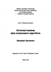
FIG. 1. A classical code is a map from a set of source objects into a set of codewords composed from an alphabet. An ensemble of source objects is mapped to an ensemble of codewords. For variable-length codes, the length of the codewords is allowed to vary.

1

Some notions and definitions are already existing, some are based on our own reasoning. When we find an already existing definition equal or similiar to the desired one, we use it and in case it is not a standard definition, we give an explicit reference. For a profound review on classical information theory, see [11,12], for a profound review on quantum information theory, see [13,14].

1

A

to be in superposition. Precisely, we interpret Ω as an orthonormal basis for a Hilbert space V and consider every normalized vector of V as a valid object. Then V is the linear span of Ω and we write V = Span(Ω) with dim V = |Ω|. The same goes for the messages. We interpret a message set M as an orthonormal basis for a message space M = Span(M ) with dim M = |M | and consider each element of M as a valid message. The map c : V → M then represents a quantum code with the space C = c(V) being the code space and the elements of C being the codewords. In order to preserve linearity, the code must be a linear map and in order to preserve norm, the code must be an isometric map. In the literature, often the code space C rather than the map c is called a code (this is a bit like calling f (x) a function). However, by saying “code” we will refer to the map c here, in full analogy to the classical case. Now let us find the general message space corresponding to the classical general message set A+ . Interpret the letters of a quantum alphabet Q as an orthonormal basis for a letter space H := Span(Q). A letter space H with k = dim H = |Q| is called a k-ary space. Quantum letters are composed into messages by tensor multiplication, giving product messages |xn i := |x1 i ⊗ · · · ⊗ |xn i that form the set Qn := {|xn i | |xi i ∈ Q} and span the block space H⊗n := Span(Qn ), giving

II. CODES

Basically, when you have a set of things and you want to give them a name, then this is a coding task. There is a code for bank accounts, telephone devices and inhabitants of a country, there even is a code for living beings: the genetic code. Language is a code for thoughts, which are in turn codes for abstract ideas or concrete objects of human experience. A code gives meaning to a message, it relates objects to their description. Objects are encoded into messages composed from a basic alphabet. The number of letters that is needed to describe a particular object is a good measure of the information content given to the object by the code. This is the key to data compression which we will study in the following with a focus on quantum codes. Classically, a code is a map c : Ω → M from a set of objects, Ω, to a set of messages, M (see Fig. 1). It is the messages that can be communicated and not the objects themselves, so communication is always based on a code. Messages (or strings) are sequences of letters taken from an alphabet A and are denoted by xn := x1 · · · xn , xi ∈ A. The empty message is denoted by x0 := ø. All messages of length n form the set An := {xn | xi ∈ A},

(1)

and the empty message forms the set A0 := {ø}. All strings of finite length form the set of general messages over the alphabet A, A+ :=

∞ [

n=0

An .

H⊗n =

(2)

n O i=1

H = H ⊗ · · · ⊗ H.

(3)

The space H⊗n is the quantum analogue to the set An of classical block messages given by (1), and contains arbitrary superpositions of product messages, which are called entangled messages. Because superposition and entanglement have no classical interpretation, quantum information is truly different from classical information. The empty message, denoted by |x0 i ≡ |øi, forms the set Q0 = {|øi} and spans the one-dimensional space H⊗0 := Span(Q0 ). Elements of H⊗n for some n ∈ N are called block messages. The set of all product S∞ messages composed from Q is denoted by Q+ := n=0 Qn . Now the general message space H⊕ induced by H can be defined by H⊕ := Span(Q+ ), giving

Every subset M ⊂ A+ is a message set. Now we can precisely define a classical k-ary code as a map c : Ω → A+ with k := |A|. The set C = c(Ω) is the codebook and each member of C is a codeword. Being a subset of A+ , a codebook is also a message set (just like a nightingale is also a bird). If C ⊂ An for some n ∈ N, then c is called a block code, otherwise a variable-length code. There is another important classification: lossless and lossy codes. A code is lossless (or uniquely decodable or non-singular ), if there are distinct codewords for distinct objects, i.e. ∀x, y ∈ Ω : x 6= y ⇒ c(x) 6= c(y). In case of a lossy code, some objects are mapped to the same encoding. Lossy codes are used when it is more important to reduce the size of the message than to ensure the correct decoding (a fine example is the MP3 code for sound data). For a given probability distribution on Ω, lossy codes can also be useful if the fidelity F , i.e. the probability of correct decoding, is close to 1. For lossless codes the fidelity is exactly 1. In this paper, we only consider lossless codes.

H⊕ =

∞ M n=0

H⊗n = H⊗0 ⊕ H ⊕ H⊗2 ⊕ · · · .

(4)

The space H⊕ is the quantum analogue to the set A+ of general classical messages given by (2). H⊕ is a separable Hilbert space with the countable basis Q+ . The space H⊕ is similiar to the Fock space in many-particle theory, except that the particles are letters here, which must be distinguishable, so there is no symmetrization or antisymmetrization. The general message space contains also superpositions of messages of distinct length,

A. The general message space

The transition from classical to quantum information is simple. We just allow the elements of a source set Ω 2

see, this additional a priori knowledge is in fact needed to make lossless compression possible. The expected length of an ensemble Σ or of the corresponding statistical message σ ∈ S(H⊕ ) is defined as X ˆ = L(Σ) = L(σ) := Tr{σ L} p(x) L(x). (10)

for example 1 √ (|101i + |11100i) ∈ H⊕ , 2

(5)

if |0i, |1i ∈ H. Any block space H⊗n is a subspace of H⊕ and is orthogonal to any other block space H⊗m with n 6= m. Elements with components of distinct length are called variable-length messages (or indeterminate-length messages) to distinguish them from block messages. Any subspace M ⊂ H⊕ is called a message space and its elements are quantum messages.

x∈X

C. Base length

The expected length of a quantum message |xi, given by (8), will in general not be the outcome of a length measurement. Every length measurement results in one of the length eigenvalues supported by |xi and generally disturbs the message. If there is a maximum value resulting from a length measurement of a state |xi, namely the length of the longest component of |xi, then let us call it the base length of |xi, defined as

B. Length operator

Define the length operator in H⊕ measuring the length of a message as ˆ := L

∞ X

n Πn ,

(6)

L(x) := max{n ∈ N | hx|Πn |xi > 0}.

n=0

For example, the quantum message

where Πn is the projector on the block space H⊗n ⊂ H⊕ , given by X Πn = |xn ihxn |. (7)

1 |xi = √ (|abrai + |cadabrai) 2

(12)

has base length 7. Since the base length of a state is the size of its longest component, we have

xn ∈Qn

ˆ is a quantum observable, the length of a message As L |xi ∈ H⊕ is generally not sharply defined. Rather, the ˆ generally disturbs the message by promeasurement of L jecting it on a block space of the corresponding length. The expected length of a message |xi ∈ H⊕ is given by ˆ L(x) := hx|L|xi.

(11)

L(x) ≥ L(x).

(13)

It is important to note that the base length is not an observable. It is only available if the message |xi is a priori known.

(8) D. Quantum code

However, in H⊕ there are also messages whose expected length is infinite. Classical analoga are probability distributions with non-existing moments, e.g. the Lorentz ˆ that distribution. Block messages are eigenvectors of L, ˆ is, L|xi = n |xi for all |xi ∈ H⊗n . The generalization to statistical ensembles is straightforward. Consider an ensemble Σ = {p, X } of variablelength messages |xi ∈ X ⊂ H⊕ occurring with probabilP ity p(x) > 0 ∀|xi ∈ X such that x∈X p(x) = 1. Then there is a density operator X σ= p(x)|xihx|, (9)

Now we can precisely define a k-ary quantum code to be a linear isometric map c : V → H⊕ , where V is a Hilbert space and H⊕ is the general message space induced by a letter space H of dimension k. The image of V under c is the code space C = c(V) (see Fig. 2). message spa e

sour e spa e

x∈X

V

ode

H

ode spa e C j01001i

alphabet

p13 (j11i + j10i + j0i)

called a statistical quantum message, representing the ensemble Σ. The set of all such density operators is denoted by S(H⊕ ). Vice versa, however, for a given density operator σ ∈ S(H⊕ ) there is in general a non-countable set of corresponding ensembles. In terms of information theory, σ cannot be regarded as a lossless code for the ensemble Σ. There is more information in the ensemble than in the corresponding density operator. As we will

p12 (j101i + j111i) p12 (j01i + j1i)

j0i j1i

3

Q

FIG. 2. A quantum code is a linear isometric map from a source space of quantum objects into a code space of codewords composed from a quantum alphabet. Superpositions of source objects are encoded into superpositions of codewords. An ensemble of source objects is mapped to an ensemble of codewords. For a variable-length quantum code, the length of the codewords is allowed to vary. Superpositions of codewords of distinct length lead to codewords of indeterminate length. The base length of a codeword is defined as the length of the longest component.

running through a wire) or some internal state with many degrees of freedom (e.g. a photon with frequency ω2 can be defined to “follow” a photon with frequency ω1 < ω2 ). The Hilbert space representing such a system of distinguishable particles with non-conserved particle number simply is the message space H⊕ . In case we have only a system at hand, where the number of particles is conserved, we can also realize variable-length messages by embedding them into block spaces. It is a good idea to distinguish between the message space, which is a purely abstract space, from its physical realization. Let us call the physical realization of a ˜ Between M message space M the operational space M. ˜ there is an isometric map, so dim M = dim M. ˜ and M, ˜ The operational space M ˜ This is expressed by M ∼ = M. is the space of physical states of a system representing valid codewords of M. Often the operational space is a subspace of the total space of all physical states of the system. Denoting the total physical space by R we have

Being a quantum analogue to the codebook, C is the space of valid codewords. The code c is uniquely specified by the transformation rule c

|ωi 7−→ |γi,

(14)

where |ωi are elements of a fixed orthonormal basis BV of V and |γi = |c(ω)i are elements of an orthonormal basis BC of C. Since c is an isometric map, i.e. hω|ω ′ i = hc(ω)|c(ω ′ )i, this implies that |c(ω)i = 6 |c(ω ′ )i ′ for all |ωi = 6 |ω i in V, so c is a lossless code with an inverse c−1 . The quantum code c can be represented by the isometric operator X X C := |c(ω)ihω| = |γihc−1 (γ)|, (15) ω∈BV

˜ ⊂ R. M∼ =M A. Bounded message spaces

The general message space H⊕ is the “mother” of all message spaces induced by the letter space H. It contains just every quantum message that can be composed using letters from H and the laws of quantum mechanics. However, it is an abstract space, i.e. independent from a particular physical implementation. It would be good to know if such a space can also physically be realized. It is clear that if you have a finite system you can only realize a finite dimensional subspace of the general message space, whose dimension is infinite. So let us start with the physical realization of the r-bounded message space

γ∈BC

called the encoder of c. Since c is lossless, there is an inverse operator X X D := C −1 = |ωihc(ω)| = |c−1 (γ)ihγ|, (16) γ∈BV

γ∈BC

called the decoder. In practice, the source space V and the code space C are often subspaces of one and the same physical space R. Since C is an isometric operator between V and C, there is a (non-unique) unitary extension UC on R with UC |xi = C|xi, UC† |yi

=C

−1

|yi,

∀|xi ∈ V ⊂ R,

∀|yi ∈ C ⊂ R.

(19)

H⊕r :=

(17) (18)

r M n=0

H⊗n ,

(20)

containing all superpositions of messages of maximal length r. Say you have a physical space R = D⊗s representing a register consisting of s systems with dim D = k. Each subspace D represents one quantum digit in the register. In the case k = 2 the quantum digits are quantum bits, in short “qbits”. The physical space R represents the space of all physical states of the register, while the message space H⊕r represents the space of valid codewords that can be held by the register and it is isomorphic to a sub˜ ⊕r of the physical space R. Let dim H = k, then space H you must choose s such that

However, using C and distinguishing between V and C is more convenient and more general. Codes with C ⊂ H⊗n for some n ∈ N are called block codes, otherwise variablelength codes.

III. REALIZING VARIABLE-LENGTH MESSAGES

Variable-length messages could in principle directly be realized by a quantum system whose particle number is not conserved, for instance, an electromagnetic field. Each photon may carry letter information by its field mode, while the number of photons may represent the length of the message. The photons can be ordered either using their spacetime position (e.g. single photons

⇒

r X

n=0

dim(H⊕r ) ≤ dim(D⊗s ) kn =

k

−1 ≤ ks k−1 ⇒

4

(21)

r+1

s ≥ r + 1.

(22) (23)

Altogether, the physical space R = D⊗(r+1) is the space of all physical states of the register, while the operational ˜ ⊕r ⊂ R is the space of those register states that space H represent valid codewords, and it is isomorphic to the abstract message space H⊕r . A general message is represented by the vector

Thus you need a register of at least (r + 1) digits to realize the message space H⊕r . Choose the smallest possible register space R = D⊗(r+1) . Since at most r digits are carrying information, one digit can be used to indicate either the beginning or the end of the message. Now you can conveniently use k-ary representations of natural numbers as codewords. Each natural number i has a unique k-ary representation Zk (i). For instance, Z2 (3) = 11 and Z16 (243) = E3. All k-ary representations have a neutral prefix “0” that can precede the representation without changing its value, e.g. 000011 ∼ = 11. For a natural number n > 0, define Zkn (i) as the n-extended k-ary representation of i by Zkn (i) := 0 · · · 0Zk (i), {z } |

0 ≤ i ≤ k r − 1.

n

|xi =

r kX −1 X

n=0 i=0

xn,i |eni i

(31)

P Pkn −1 with rn=0 i=0 |xn,i |2 = 1. The length operator introduced in section II B is here of the form r X ˆ L := n Πn , (32)

(24)

n=0

n

For example, = 000011 and = 0000E3. Let us define that the message starts after the first appearance of “1”, e.g. 000102540 ∼ = 02540. Now define orthonormal vectors

because there are at most r digits to constitute a message. Now we need to know how the projectors Πn are ˜ ⊕r . For a register constructed in the operational space H state containing a message of sharply defined length, the length eigenvalue n is given by the number of significant digits in that register,

|eni i := | 0| ·{z · · 0} 1Zkn (i)i ∈ R

ˆ |eni i := n |eni i, L

Z26 (3)

6 Z16 (243)

(25)

r−n

n

for 0 ≤ i ≤ k − 1. Each projector is then defined by

where n > 0 and 0 ≤ i ≤ k n −1. The n digits of Zkn (i) are called significant digits. The empty message corresponds to the unit vector |øi := |e00 i := |0 · · · 01i.

Πn :=

(26)

|eni iheni |

(34)

and projects onto the space H⊗n ⊂ R. Note that the physical length of each message is always given by the fixed size (r + 1) of the register. Only the significant length of a message, i.e. the number of digits that constitute a message contained in the register, is in general not sharply defined. Note further that the particular form of the length operator depends on the realization of the message space. In the limit of large r we have lim H⊕r = H⊕ , but r→∞ that space can no longer be embedded into a physical space R = D⊗∞ := lim D⊗n , since the latter is no sepn→∞ arable Hilbert space anymore. However, we can think of r as very large, such that working in H⊕ just means working with a quantum computer having enough memory.

register 0 0 0 0 0 1 0 7 3 significant digits

start digit

FIG. 3. Realizing a general variable-length message.

Next, define orthonormal basis sets  B˜n := |en0 i, . . . , |enkn −1 i}, 0 ≤ n ≤ r,

n kX −1

i=0

Obviously, |øi has no significant digits.

redundant digits

(33)

(27)

that span the operational block spaces ˜ ⊗n = Span(B˜n ). H

B. Realizing more message spaces

(28)

˜ ⊗n is truly different from H⊗n , because H ˜ ⊗n Note that H r+1 ⊗n n ˜ has dimension k , while H has dimension k . Next, define an orthonormal basis B˜+ :=

r [

n=0

B˜n ,

A code is a map c : V → H⊕ from source states in V to codewords in H⊕ . The space C = c(V) of all codewords is the code space and as a subspace of the general message space H⊕ it is just a special message space. In order to implement a particular code c, it is in practice sufficient to realize only the corresponding code space C by a physical system. Let us realize some important code spaces now. However, we will not discuss the very important class of error-correcting code spaces here, since this would go beyond the scope of this paper.

(29)

˜ ⊕r ⊂ R by and construct the operational space H ˜ ⊕r := Span(B˜+ ). H

(30) 5

1. Block spaces

3. Neutral-prefix space

An important message space is the block space H⊗n , that contains messages of fixed length n. Block spaces are the message spaces of standard quantum information theory. They can directly be realized by a register R = H⊗n of n digits, e.g. n two-level systems representing one qbit each.

A specific code space will be of interest, namely the space of neutral-prefix codewords, which we define as follows. The k-ary representation of a natural number i is denoted by Zk (i) (see section III A). The empty message ø is represented by Zk (0) = ø. Define an orthonormal basis Br := {|Zk (0)i, . . . , |Zk (k r − 1)i}

2. Prefix spaces

of variable-length messages of maximal length r. The length of each basis message |Zk (i)i is given by

Another interesting message space is the space of prefix codewords of maximal length r. Such a space contains only superpositions of prefix codewords. A set of codewords is prefix (or prefix-free), if no codeword is the prefix of another codeword. For example, the set P3 = {0, 10, 110, 111} is a set of binary prefix codewords of maximal length 3. Prefix codewords have one significant advantage:

|Zk (i)| = ⌈logk (i + 1)⌉,

(37)

where ⌈x⌉ denotes the smallest integer ≥ x. These basis messages span the r-bounded neutral-prefix space Nr := Span(Br ).

(38)

Note that Nr is not equal to the r-bounded message space H⊕r as you can see by comparing the dimension r+1 dim Nr = k r with dim H⊕r = k k−1−1 . Nr is smaller than H⊕r , because not all messages of H⊕r are contained in Nr . For example, the message |01i is in H⊕r but not in Nr , hence we have

• Prefix codewords are instantaneous, that is, sequences of prefix codewords do not need a word separator. The separator can be added while reading the sequence from left to right. A sequence from P3 can be separated like 110111010110 7→ 110, 111, 0, 10, 110.

(36)

(35)

Nr ⊂ H⊕r .

(39)

Now we want to find a physical realization of Nr . This turns out to be quite easy (see Fig. 4).

However, there is also a drawback: • Prefix codewords are in general not as short as possible.

register

This is a consequence of the fact that there are in general less prefix codewords than possible codewords. For example, if you want to encode 4 different objects, you can use the prefix set P3 above with maximal length 3. If you renounce the prefix property you can use the set {0, 1, 01, 10} with maximal length 2. A prefix space Pr of maximal length r is given by the linear span of prefix codewords of maximal length r. For the set P3 , the corresponding prefix space is P3 = Span{|0i, |10i, |110i, |111i}. The prefix space Pr ⊂ H⊕r can physically be realized by a subspace P˜r of the register space R = D⊗r spanned by the prefix codewords which have been extended by zeroes at the end to fit them into the register. For example, P˜3 = Span{|000i, |100i, |110i, |111i} ⊂ D⊗3 is a physical realization of the prefix space P3 . The length operator measures the significant length of the codewords, given by the length of the corresponding prefix codewords. Schumacher and Westmoreland [8] as well as Braunstein et al. [6] used prefix spaces for their implementation of variable-length quantum coding. However, we will show later on that the significant advantage of prefix codewords in fact vanishes in the quantum case, whereas the disadvantage remains.

0 0 0 0 0 1 0 7 3 redundant digits

significant digits

FIG. 4. Realizing variable-length messages by neutral-prefix codewords.

As already noted in section III A, the k-ary representation Zk (i) of any natural number i can be extended by leading zeroes to the r-extended k-ary representation Zkr (i) := 0 · · · 0Zk (i). Take a register R = D⊗r of r digits with D = Ck . Then the set BR := {|Zkr (0)i, . . . , |Zkr (k r − 1)i}

(40)

is an orthonormal basis for the register space R. At the same time it can be regarded as an orthonormal basis for the operational space N˜r representing the neutral-prefix space Nr . While the physical length of each codeword is constantly r, the significant length is measured by the length operator ˆ := L

r X

n=0

6

n Πn ,

(41)

with mutually orthogonal projectors X |Zkr (i)ihZkr (i)|. Πn :=

Note that the so-defined length operator looks different ˆ is always from the one defined in section III A. While L of the same form (32), the projectors Πn are different because the operational spaces are different. The empty message can be defined by

up to 50,000 letters representing a manifold of abstract and concrete things, e.g. the “noise of a running horse”. The length of the code is minimized to 1, but the encoding and decoding machines will need a large memory to remember all the letters. Obviously, a raw code does not compress at all, so it is a good idea to set the effort of communication in relation to the raw information content of Ω (similiar notion in [14] p.71, and interestingly similiar also to the Boltzman entropy of a microcanonical ensemble), defined by

|øi := |Zkr (0)i = |0 · · · 0i.

I0 (Ω) := log2 |Ω|.

(42)

i: |Zk (i)|=n

(43)

A general message in N˜r is given by |xi =

r kX −1

i=0

xi |Zkr (i)i.

(45)

I0 (Ω) represents the number of binary digits (bits) needed to enumerate the elements of Ω. This motivates the following definition. The code information content of an individual object in an arbitrary set Ω for a given k-ary code c : Ω → A+ is defined as

(44)

We have realized the neutral-prefix space Nr by exhausting the entire register space R, so the quantum resources are optimally used. In other words:

Ic (x) := log2 k · Lc (x),

x ∈ Ω,

(46)

where Lc (x) denotes the length of the codeword c(x) ∈ A+ . Ic (x) represents the number of bits needed to describe the object x by the code c. For a raw code c : Ω → A, definition (46) gives the raw information content for every object x ∈ Ω. A few remarks about the code information: 1) The code information is defined for things, not for strings. Of course, things may sometimes also be strings. If so, one can define the direct information of a string xn over an alphabet A as

• All messages in Nr are as short as possible. Remember that the physical realization of H⊕r requires one additional digit to represent the beginning or the end of a message. This digit does not contain any message information, it is sort of wasted. For quantum coding, the additional digit may really count, since it would have to be added each time a codeword is stored or transmitted! Also the prefix space considered in section III B 2 contains messages which are not as short as possible. You can encode a space V of dimension dim V = 4 by a prefix space spanned by {|000i, |100i, |110i, |111i} with corresponding lengths {1, 2, 3, 3}, but then you need a register of 3 qbits. In contrast to that, V can be encoded by a neutralprefix space spanned by the basis {|00i, |01i, |10i, |11i} with corresponding lengths {0, 1, 2, 2}, and you need a ˜r , the register of only 2 qbits. In the operational space N basis messages reveal their length information by simply discarding leading zeroes. That way, not all variablelength messages can be realized, but we save 1 register digit, so Nr is a good candidate for variable-length quantum coding.

I(xn ) := n log2 |A|.

(47)

2) The code information Ic is code dependent, reflecting the philosophy that there is no information contained in an object without a code giving it some meaning. The codeword ”XWF$%&$ FggHz((” may be a random sequence of letters or may in a certain code represent the first digits of π or in another code the beginning of a Mozart symphony. Now let there be a probability distribution p on Ω. We can define the code information of the ensemble Σ = {p, Ω} as the average of (46), Ic (Σ) := log2 k

IV. DATA COMPRESSION

X

p(x) Lc (x).

(48)

x∈Ω

Compression means reducing the code information of the ensemble. We can define the compression rate achieved by a code c on the ensemble Σ by

A. Classical data compression

Intuitively, compression is achieved when the effort to store or communicate the codewords is minimized. But how can we precisely define that “effort”? The key idea is the concept of a raw code. One can always construct a code for Ω by inventing a new letter for each single object. Such a classical raw code is a code c : Ω → A for some alphabet A of the same size as Ω. The chinese writing is a fairly good illustration of a raw code. There are

Rc (Σ) :=

Ic (Σ) , I0 (Ω)

(49)

A code c : Ω → C is compressive on Σ if and only if Rc (Σ) < 1 i.e. Ic (Σ) < I0 (Ω). 7

(50)

Ic (x) = hx|Iˆc |xi that is found by performing a length measurement on the codeword for |xi. In the classical case, the difference vanishes. Now suppose you want to encode an ensemble Σ = {p, X } of states |xi ∈ X that span the source space V. Each individual message |xi can be compressed to I c (x) qbits, so the entire ensemble Σ will on the average be compressed to the code information X p(x) Lc (x). I c (Σ) := log2 k (56)

B. Quantum data compression

Now that we have a classical definition of compression, the next step is to translate these concepts to the quantum case. Again, the key is the raw information, i.e. the size of a non-compressed message, so let us look for its quantum analogue. The raw information (45) of a set Ω is I0 (Ω) = log2 |Ω| because we need |Ω| distinct letters to encode each element of Ω by a raw code. Interpreting Ω as an orthonormal basis for a Hilbert space V, the raw information of V is also log2 |Ω|, because we still need |Ω| distinguishable letters to represent each element of the space V. Since |Ω| = dim V, we define the quantum raw information of a space V as I0 (V) := log2 (dim V).

x∈X

The compression rate can then be defined by Rc (Σ) :=

(51)

Rc (Σ) < 1 i.e. I c (Σ) < I0 (V).

(52)

V. NO-GO THEOREMS

Of course, lossy compression is always possible. But let us look for some statements about lossless codes. The first three of the following no-go theorems are also known in classical information theory and are easily transferred to the quantum case by general reasoning. However, we show them by applying the tools developped in this paper. The last theorem is genuinely quantum with no classical analogue.

(53)

In short, the code information operator is defined in an arbitrary Hilbert space V and depends on a quantum code c : V → H⊕ , while the direct information operator is defined in a message space H⊕ without referring to a quantum code. For a given code, the relation between both operators is Iˆc = C −1 Iˆ C.

(58)

Note that these definitions only apply to lossless codes. The lossy case is not considered here.

ˆ c := C −1 L ˆ C is the length operator measuring where L the length of the codeword for a source vector in V. If the code is based on a qbit alphabet, Iˆc measures the number of qbits forming the code message, hence the measuring unit of Iˆc is “1 qbit”. In analogy to (47), we define the direct information operator acting on the message space H⊕ by ˆ Iˆ := log2 k · L.

(57)

A code c is compressive on the ensemble Σ, if and only if

So the quantum raw information I0 corresponding to a space V equals the fixed number of qbits needed to represent all states in V. Now, for a given k-ary code c : V → H⊕ represented by an encoder C, the code information operator can be defined as ˆ c, Iˆc := log2 k · L

I c (Σ) . I0 (V)

A. No lossless compression by block codes

A code is a block code if all codewords have the same length, else it is a variable-length code. Unfortunately, lossless block codes do not compress. Take an arbitrary ensemble Σ = {p, X } with X ⊂ V and any lossless k-ary block code c : V → H⊗n . Let BV and Bn be orthonormal basis sets of V and H⊗n , respectively. In order to find for every basis vector |ωi ∈ BV a code basis vector |c(ω)i ∈ Bn , the code must fulfill dim V ≤ dim H⊗n = k n . For every |xi ∈ X , the corresponding codeword |c(x)i has sharp length L(x) = n, hence X I c (Σ) = log2 k p(x) Lc (x) = log2 k · n = log2 (k n ) (59)

(54)

Now you want to compress a codeword by removing redundant quantum digits. The number of quantum digits carrying information is given by the base length of the codeword. All other digits are redundant and can be removed without loss of information. This motivates the definition of the code information of a state |xi ∈ V respecting a code c by

x∈X

I c (x) := log2 k · Lc (x),

≥ log2 (dim V) = I0 (V),

(55)

(60)

which violates condition (58). This implies that there is no lossless compressing block code. By choosing mutually orthogonal source states one can derive the analogue statement for the classical case.

where Lc (x) = L(c(x)) is the base length of the codeword for |xi. I c (x) represents the number of qbits needed to describe the state |xi by the code c. This value must be distinguished from the expected number of qbits 8

have a space H⊕r of variable-length messages with maximal length r. Assume that there is a universal lossless code c that reduces the length of all messages in H⊕r . The code can only be lossless if dim H⊕r ≤ dim H⊕s , which is obviously wrong for r > s, so you cannot compress all variable-length messages with a given maximal length. Concluding, there is no universal lossless compression that reduces the size of all messages. Some messages are unavoidably lengthened by a lossless code. By choosing mutually orthogonal source states, one can derive the analogue statement for the classical case.

For long strings emitted by a memoryless source, block codes can achieve almost lossless compression by encoding only typical subspaces. The quantum code performing this type of lossy compression is known as the Schumacher code [3]. The only way to compress messages without loss of information is by use of a variable-length code. In order to achieve compression, more frequent objects must be encoded by shorter messages, less frequent objects by longer messages, so that the average length of the codes is minimized. This is the general rule of lossless data compression.

B. No lossless compression by changing the alphabet D. No lossless compression of unknown messages

Trying to achieve compression by using a different alphabet does not work. ⊗n ⊗m → HB that transforms messages A code c : HA over some letter space HA into messages over some letter ⊗n ⊗m space HB is lossless only if dim HA ≤ dim HB , which implies that I0 (V) = n log2 (dim HA ) ≤ m log2 (dim HB ) = I c (x),

Now we come to a no-compression theorem that is typically quantum. In quantum mechanics there is a profound difference between a known and an unknown state. For example, a known state can be cloned (by simply preparing another copy of it), whereas an unknown state cannot be cloned. Assume that there is a lossless quantum compression algorithm c : H⊗r → H⊕s that compresses messages of fixed length r to variable-length messages of maximal length s. As we have seen in the last section, a lossless code cannot compress all messages, so s > r. Now there isPan oracle that hands you an arbitrary message n |xi = i=1 xi |ωi i where the |ωi i ∈ H⊕r are mutually orthogonal states.PThe algorithm encodes the message n |xi into |c(x)i = i=1 xi |c(ωi )i. Even if all the codeword components |c(ωi )i have determinate length Lc (ωi ), the total codeword |c(x)i has in general indeterminate length. If you want to remove redundant digits without loss of information, you must know at least an upper bound for its base length, i.e. the length of its longest component. Since you do not know the source message |xi, you do not know the base length of its encoding |c(x)i, so you have to assume the maximal length s. Since s > r, no compression is achieved. The same argument applies to quantum compression algorithms c : H⊕r → H⊕s compressing variable-length messages of maximal length r to variable-length messages of maximal length s. We conclude that lossless compression of unknown quantum messages is in general impossible. This statement is not true for the classical case. A classical message is not disturbed by a length measurement, so it can in principle be compressed without loss of information. It would have been nice to compress a quantum hard disk without loss of information just like a classical hard disk, but this cannot be accomplished in general. Now that we have found a lot of impossible things to do with quantum messages, it is time to look for the possible things.

(61) (62)

for every |xi ∈ HA . So for every ensemble Σ = {p, X } m of messages |xi ∈ HA , we have I c (Σ) = I c (x) ≥ I0 (V), which violates condition (58). By choosing mutually orthogonal source states, one can derive the analogue statement for the classical case. This paper looks probably much shorter when written in chinese symbols. However, the effort of communication that is expressed by the code information Ic , would not be reduced.

C. No universal lossless compression

We have seen that it is not possible to compress messages without loss of information by using a block code or by using a different letter space. Now we will see that no code can compress all messages without loss of information. Say you have a space H⊗n of block messages of fixed length r and you want to compress all of them by use of a variable-length code c : H⊗r → H⊕s with s < r. The code can only be lossless if dim H⊗r ≤ dim H⊕s . But since dim H⊗r = k r and dim H⊕s = k s+1 − 1 k−1 ≤ k s+1 + k − 1

kr ≤ ⇒

k r+1

(63) ks+1 −1 k−1 ,

we have (64) (65)

which is wrong for r ≥ s and k > 1, so you cannot compress all block messages of a given length. Now say you 9

that does not fix the problem. Whatever one does, reading out length information about different components of a variable-length codeword equals a length measurement and hence means disturbing the message. Though there should be some way to make sure where the codewords have to be separated, else the message cannot be decoded at all. Here is an idea: Use a classical side-channel to inform the receiver where the codewords have to be separated. This has two significant advantages:

VI. LOSSLESS COMPRESSING CODES

The intention of using compressing codes is to minimize the effort of communication between two parties: one who prepares, encodes, compresses and sends the messages and one who receives, decompresses, decodes and possibly reads them. So it’s time for Alice and Bob to enter the scene. Alice is preparing source messages |xi ∈ V and encodes them into codewords |c(x)i ∈ H⊕r by applying the encoder C. She compresses the codewords by removing redundant quantum digits and sends the result to Bob, who receives them and decompresses them by appending quantum digits. After that he can decode the messages by applying the decoder D and read them or use them as an input for further computations. The communication has been lossless, if the decoded message equals the source message. Note that it is not required for Bob to read the message he received! In fact, if Bob wants to use the message as an input for a quantum computer, he even must not do that, else he will potentially lose information. We require Alice to know which source messages she prepares, otherwise no lossless compression is possible, as we have seen in the previous section.

• If the length information equals the base length of the codeword, the message is not disturbed and can be losslessly transmitted and decoded. • Abandoning the prefix condition, shorter codewords can be chosen, such that the quantum channel is used with higher efficiency. Quantum Channel ...

+ j1101i + j10i

Classical Channel

7

FIG. 5. Storing side-channel.

A. Why prefix quantum codes are not very useful

j1001101i

length

j11i

j10i

+ j1011i + j11i + j11101i + j1i 5

information

...

2

in

a

classical

Let us give an example (see Fig. 5). Alice wants to send a message |x1 i which is encoded into the codeword |c(x1 )i = √13 (|1001101i + |1101i + |10i). The base length of |c(x1 )i is 7, so she submits that information through the classical channel. Dependent on which realization of variable-length messages Alice and Bob have agreed to use, Alice sends enough qbits (at least 7) representing the codeword |c(x1 )i through the quantum channel. The next codeword is |c(x2 )i = √13 (|11i + |1011i + |11101i). The base length of |c(x2 )i is 5, so Alice sends the length information “5” through the classical channel and enough qbits (at least 5) representing the codeword |c(x2 )i through the quantum channel. She proceeds like that with all following messages. On Bob’s side, there is a continuous stream of qbits coming through the quantum channel and a continuous stream of classical bits coming through the classical channel. Bob can read out the classical length information, separate the qbits into the specified blocks and apply the decoder to each codeword. After all, Bob obtains all source messages without loss of information.

In classical information theory, prefix codes are favored for lossless coding. The reason is that they are instantaneous, which means that they carry their own length information (see section III B 2). Prefix codewords can be sent or stored without a separating signal between them. The decoder can add word separators (“commas”) while reading the sequence from left to right. Whenever a string of letters yields a valid codeword, the decoder can add a comma and proceed. After all, a continuous stream of letters is separated into valid codewords. Prefix codewords can be separated while reading the sequence, but in the quantum case this is potentially a very bad thing to do. Reading a stream of quantum letters means in general disturbing the message all the time. Therefore, the length information is generally not available. Furthermore, prefix codewords are in general longer than non-prefix codewords, because there are less prefix codewords of a given maximal length than possible codewords. Hence, by using prefix codewords qbits are wasted to encode length information which is unavailable anyway. We conclude that prefix quantum codes are practically not very useful.

C. How much compression? B. A classical side-channel

1. Lower bound

One could try to encode length information in a different quantum channel, as proposed by Braunstein et al. [6] (unnecessarily they used prefix codewords anyhow). But

How much compression can maximally be achieved by using the method sketched in section VI B? Say Alice has an ensemble Σ = {p, X } of m = |X | messages |xi i ∈ X , 10

i = 1, . . . , m that she wants to encode by k-ary codewords. The source space V is spanned by the elements of X , thus V := Span(X ), and has dimension d := dim V. Alice fixes a basis set BV of d orthonormal vectors |ωi i, i = 1, . . . , d. The ensemble Σ corresponds to the message matrix σ :=

m X i=1

p(xi ) |xi ihxi | =

d X

i,j=1

σij |ωi ihωj |,

just like all uniquely decodable symbol codes, have to fulfill the Kraft inequality [11,12] d X i=1

|ωi i 7−→ |c(ωi )i,

i = 1, . . . d.

(66)

ˆ

TrV {k −Lc′ } ≤ 1,

ˆc = L

i=1

ˆlc′ :=

(67)

(68)

Lc (Σ) = ≥ =

i=1

m X

(70)

ˆ c |xi i = Tr{σ L ˆc} p(xi ) hxi |L

(71)

(77)

1 −Lc (ωi )−lc′ (ωi ) k , Q

(78)

which can be rewritten as Lc (ωi ) = − logk q(ωi ) − logk Q − l′ (ωi ).

(79)

Summing over the σii yields d X i=1

σii Lc (ωi ) = −

d X i=1

σii logk q(ωi ) − logk Q − l′ , (80)

where l′ :=

d X i=1

σii lc′ (ωi ) = Tr{σ ˆlc′ }

(81)

is the average additional length. The inequality (72) can now be expressed by Lc (Σ) ≥ −

(72)

i=1

d X i=1

σii logk q(ωi ) − logk Q − l′

(82)

Gibbs’ inequality implies that

Now we perform the following trick. As already stated, non-prefix codewords can be chosen shorter than (or at most as long as) prefix codewords. Consider an arbitrary prefix code c′ , then Lc′ (ωi ) = Lc (ωi ) + lc′ (ωi ) ≥ Lc (ωi ),

k −Lc (ωi )−lc′ (ωi ) ≤ 1.

q(ωi ) :=

(69)

p(xi ) Lc (xi )

σii Lc (ωi ).

(76)

Now define implicit probabilities

i=1

m X

d X i=1

Now we are interested in the average base length, since this determines the compression rate. The average base length is bounded from below by m X

lc′ (ωi ) |ωi ihωi |.

The quantum Kraft inequality was derived for the first time by Schumacher and Westmoreland [8]. Here, the quantum Kraft inequality requires that

The codewords |c(ωi )i are not necessarily prefix, because Alice can encode the length information about each codeword in a classical side-channel. In order for the transmission to be lossless, she has to transmit the base length Lc (xi ) of each codeword corresponding to the source message |xi i. The base length is at least as long as the expected code length of the codeword, hence ˆ c |xi i. Lc (xi ) ≥ hxi |L

d X i=1

Q := Lc (ωi ) |ωi ihωi |.

(75)

ˆ c′ := L ˆ c + ˆlc′ and where L

The code space is k-ary, which means that k = dim H. Let each codeword |c(ωi )i have determinate length ˆ c on V is Lc (ωi ), such that the code length operator L orthogonal in the basis BV and reads d X

(74)

ˆ c′ is orthogonal in the Since the code length operator L basis BV , we can express the above condition by the quantum Kraft inequality

Pd with σij := hωi |σ|ωj i and i=1 σii = 1. The source messages are encoded by the isometric map c : V → H⊕ , defined by c

k −Lc′ (ωi ) ≤ 1.

Lc (Σ) ≥ −

d X i=1

σii logk σii − logk Q − l′ .

(83)

The von-Neumann entropy of the message matrix σ cannot decrease by a non-selective projective measurement in the basis BV , hence

(73)

where lc′ (ωi ) ≥ 0 is the length difference between the prefix and the non-prefix codeword for |ωi i. Prefix codes,

S(σ) ≤ S(σ ′ ), 11

(84)

where σ ′ :=

D. Quantum Morse codes d X i=1

|ωi ihωi |σ|ωi ihωi | =

d X i=1

σii |ωi ihωi |.

(85)

Since S(σ ′ ) = −

d X i=1

σii log2 σii = − log2 k

d X

σii logk σii , (86)

i=1

relation (84) states that −

d X i=1

σii logk σii ≥

1 S(σ). log2 k

(87)

Using (87) together with the Kraft inequality Q ≤ 1, relation (83) transforms into  (88) log2 k · Lc (Σ) + l′ ≥ S(σ) − logk Q ≥ S(σ). Recalling the definition of the code information (56) and defining the length information that can be drawn into the classical side-channel by I ′ := log2 k · l′ ,

One way to avoid a classical side-channel is to leave a pause between the quantum codewords, which equals an additional orthogonal “comma state”. Such a code is a quantum analogue to the Morse code, where the codewords are also separated by a pause, in order to avoid prefix codewords. Of course, the codewords plus the pause are prefix. Due to the close analogy one could speak of quantum Morse codes. Here, the information I ′ needed for the comma state is independent from the statistics, because the comma state must be sent after each letter codeword, no matter which one. In contrast to that, I ′ is in general dependent from the statistics. If one transmits the length of each codeword through a classical side-channel, one can use a Huffman code to find shorter codewords for more frequent length values. Such is done in the following compression scheme.

(89)

VII. A LOSSLESS COMPRESSION SCHEME

(90)

Let us construct an explicit coding scheme that realizes lossless quantum compression.

we finally arrive at the lower bound relation I c (Σ) + I ′ ≥ S(σ).

If c is a uniquely decodable symbol code, e.g. a prefix code, we have I ′ = 0. Inequality (90) states that the ensemble Σ can be losslessly compressed not below S(σ) qbits. However, by drawing length information into a classical side-channel it is possible to reduce the average number of qbits passing through the quantum channel below the von-Neumann entropy. We will give an example later on where this really happens.

A. Preparations

Alice and Bob have a quantum computer on both sides of the channel. They both allocate a register of r kary quantum digits, whose physical space is given by R = D⊗r with D = Ck . They agree to use neutral-prefix codewords (see section III B 3) to implement variablelength coding, hence the message space is Nr of dimension k r and is physically realized by the operational ˜r = R. Alice is preparing source messages space N |xi i, i = 1, . . . , m from a set X . The space spanned by these messages is the source space V = Span(X ). Alice prepares each message |xi ∈ X with probability p(x), which gives the ensemble Σ := {p, X }. She encodes the source messages into variable-length codewords |c(x)i ∈ Nr of maximal length r. If the dimension of V is given by d := dim V, then the length of the register must fulfill

2. Upper bound

Let us look for an upper bound for the compression that can be achieved. In order to encode every source vector in V by a k-ary code, we need at most Lc (x) ≤ ⌈logk (dim V)⌉ ≤ logk (dim V) + 1

(91)

digits. Using loga x = loga b · logb x, we have I c (Σ) ≤ log2 (dim V) + log2 k.

(92)

This upper bound is neither very tight nor is it related to the von-Neumann entropy. However, our efforts to find a more interesting upper bound were not successful. It remains an open question to find such a bound and hence a quantum mechanical generalization to Shannon’s theorem [15], H(Σ) ≤ Ic (Σ) ≤ H(Σ) + log2 k,

r ≥ ⌈logk d⌉.

(94)

If the set X is linearly dependent, Alice creates a set X˜ = X , removes the most probable message from X˜ and puts it into a list M . Next, she removes again the most probable message from X˜ , appends it to the list M and checks if the list is now linearly dependent. If so, she

(93)

which looks more familiar for k = 2, such that log2 k = 1 and Ic (Σ) = Lc (Σ). 12

removes the last element from M again. Then she proceeds with removing the next probable message from X˜ and appending it to M , checking for linearly dependence, and so on. In the end she obtains a list M = (|x1 i, . . . , |xd i)

B. Communication protocol

(95) Alice prepares the message |xi ∈ X and applies the encoder C to obtain |c(x)i. She looks up the corresponding code base length Lc (x) in the table. If Lc (x) < r, she truncates the message to Lc (x) digits by removing r − Lc (x) leading digits. She sends the Lc (x) digits through the quantum channel and the length information Lc (x) through the classical channel. Then she proceeds with the next message.

of linearly independent source messages from X , ordered by decreasing probability, such that p(xi ) ≥ p(xj ) for i ≤ j. She performs a Gram-Schmidt orthononormalization on the list M , giving a list B of orthornormal vectors |ωi i, defined by |ω1 i := |x1 i, i−1 i h X |ωj ihωj | |xi i, |ωi i := Ni 1 −

(96)

For any message |xi Alice sends, Bob receives the length information Lc (x) through the classical channel and Lc (x) digits through the quantum channel. He adds r − Lc (x) quantum digits in the state |0i at the beginning of the received codeword. He then applies the decoder D and obtains the original message |xi with perfect fidelity. Note that Alice can send any message from the source message space V, the protocol will ensure a lossless communication of the message. For such arbitrary messages, however, compression will in general not be achieved, since the protocol is only adapted to the particular ensemble Σ. Also, Bob can as well store all received quantum digits on his quantum hard disk and the received length information on his classical hard disk, and go to bed. The next day, he can scan the classical hard disk for length information and separate and decode the corresponding codewords on the quantum hard disk. The protocol works as well for online communication as for data storage.

(97)

j=1

with i = 2, . . . , d and suitable normalization constants Ni . The elements of B form an orthonormal basis BV for the source space V. Now she assigns codewords |c(ωi )i := |Zkr (i − 1)i,

i = 1, . . . , d.

(98)

of increasing significant length Lc (ωi ) = ⌈logk (i)⌉.

(99)

Note that the first codeword is the empty message |øi = |Zkr (0)i = |0 · · · 0i, which does not have to be sent through the quantum channel at all. Instead, nothing is sent through the quantum channel and a signal representing “length 0” is sent through the classical channel. Alice implements the encoder C :=

d X i=1

|c(ωi )ihωi |,

(100)

by a gate array on R. Then she calculates the base lengths of the codewords, 2

Lc (x) = max {Lc(ωi ) | |hωi |xi| > 0}, i=1,... ,d

C. An explicit example

(101)

for every message |xi ∈ X and writes them into a table. The classical information is compressed using Huffman coding of the set of distinct base length values L = {Lc (ω1 ), . . . , Lc (ωd )}. Alice constructs the Huffman codeword to each length l ∈ L appearing with probability pl =

X

p(x),

Alice and Bob want to communicate vectors of a 4dimensional Hilbert space V = Span{|0i, |1i, |2i, |3i}, where we use the row notation in the following. Alice decides to use the (linearly dependent) source message set

(102)

x: Lc (x)=l

and writes them into a table. At last, Alice builds a gate array realizing the decoder D = C −1 and gives it to Bob. For the classical channel she hands the table with the Huffman codewords for the distinct lengths to Bob. Now everything is prepared and the communication can begin.

X = {|ai, |bi, |ci, |di, |ei, |f i, |gi, |hi, |ii, |ji}, whose elements are given by 13

(103)

|ai = |bi = |ci = |di = |ei = |f i = |gi = |hi = |ii = |ji =

1 (1, 1, 1, 1) 2 1 √ (1, 2, 1, 1) 5 1 √ (1, 3, 1, 1) 6 1 √ (1, 4, 1, 1) 7 1 √ (1, 0, 1, 0) 2 1 √ (2, 0, 1, 0) 3 1 (3, 0, 1, 0) 2 1 √ (0, 1, 0, 1) 2 1 √ (0, 2, 0, 1) 3 1 (0, 3, 0, 1) 2

Let the quantum channel be binary, i.e. let k = 2. The codewords are constructed along |c(ωi )i = |Z2 (i − 1)i, yielding the variable-length states

(104) (105)

|c(ω1 )i = |øi |c(ω2 )i = |1i |c(ω3 )i = |10i |c(ω4 )i = |11i,

(106) (107) (108)

that span the code space C. In a neutral-prefix code they are realized by the 2-qbit states

(109)

|˜ c(ω1 )i = |00i |˜ c(ω2 )i = |01i |˜ c(ω3 )i = |10i |˜ c(ω4 )i = |11i

(110) (111)

˜ which is a subthat span the operational code space C, 2 space of the physical space RP= C ⊗ C2 . Alice realizes ˜ C= c(ωi )ihωi |, given by the encoder C : V → C, i |˜

(113)

and which are used with the probabilities p(b) = p(c) = p(d) = 0.1, 0.3 p(e) = . . . = p(j) = . 3

 0.5 0.5 0.5 0.5 −0.288675 0.866025 −0.288675 −0.288675 C= 0.408248 0 0.408248 −0.816497 0.707107 0 −0.707107 0 (134) 

(115) (116)

The Shannon entropy of the ensemble Σ = {p, X } is H(Σ) = 2.02945,

and the decoder D = C −1 , given by

(117)

and the classical raw information (45) reads I0 (X ) = log2 |X | = 3.32193,

  0.5 0.408248 −0.288675 0.707107 0 0.866025 0  0.5 (135) D= 0.5 0.408248 −0.288675 −0.707107 0.5 −0.816497 −0.288675 0

(118)

which gives an optimal classical compression rate of R = H/I0 = 0.610924. If Bob knows Alice’s list of possible messages, then this rate could in the optimal case be achieved by pure classical communication. However, Bob does not know the list and classical communication is not P the task here. The message matrix σ = x∈X p(x)|xihx|, given by   0.214549 0.224624 0.197882 0.177882 0.224624 0.40302 0.224624 0.244624 (119) σ= 0.197882 0.224624 0.191216 0.177882 0.177882 0.244624 0.177882 0.191216

by gate arrays and gives the decoder to Bob. The encoded alphabet is obtained by |c(x)i = C|xi. Alice writes the base lengths of the codewords Lc (a) = 0, Lc (b) = Lc (c) = Lc (d) = 1, Lc (e) = . . . = Lc (j) = 2

p0 = 0.6,

p1 = 0.3,

p2 = 0.1

(138)

She constructs Huffman codewords for each length

(120)

The orthogonalization procedure yields the basis BV = {|ωi i} with |ω1 i = (0.5, 0.5, 0.5, 0.5) |ω2 i = (−0.288675, 0.866025, −0.288675, −0.288675) |ω3 i = (0.408248, 0, 0.408248, −0.816497) |ω4 i = (0.707107, 0, −0.707107, 0).

(136) (137)

in a table and calculates the corresponding probabilities

has von-Neumann entropy S(σ) = 0.571241.

(129) (130) (131) (132) (133)

(112)

(114)

p(a) = 0.6,

(125) (126) (127) (128)

c0 = 1,

c1 = 01,

c2 = 00,

(121) such that the average bit length is (122) 2 X (123) L′ = pl · l = 1.4, l=0 (124) 14

(139)

(140)

In other words, the number of qbits passing through the quantum channel is reduced by 75 %. Sending 100 messages without compression requires 200 qbits. Using the compression scheme, Alice typically sends 50 qbits. c. The sum of both quantum and classical information,

which is the optimal value next to the Shannon entropy of the length ensemble ′

I =−

2 X

pl log2 pl = 1.29546 .

(141)

l=0

Alice hands the table with the Huffman codewords to Bob and tells him that he must listen to the classical channel, decode the arriving Huffman codewords into numbers, receive packages of qbits, whose size corresponds to the decoded numbers, and add to each package enough leading qbits in the state |0i to end up with 2 qbits. Then he must apply the decoder D to each extended package and he will get Alice’s original messages. Say, Alice wants to send the message |ai. She prepares |ai and applies the encoder C to obtain the codeword |00i. She looks up the corresponding base length Lc (a) = 0 and truncates the codeword to Lc (a) = 0 qbits. In this case there are no qbits left at all, so she sends nothing through the quantum channel and the Huffman codeword for “length 0” through the classical channel. Bob receives the classical length information “0” and knows that nothing comes through the quantum channel and that in this case he has to prepare 2 qbits in the state |00i. He applies the decoder D and obtains Alice’s original message |ai. In order to send message |bi, Alice truncates the codeword to Lc (b) = 1 qbit and obtains √12 (|0i + |1i). She sends the qbit through the quantum channel together with the classical signal “length 1”. Bob receives the length message and knows that he has to take the next qbit from the quantum channel and that he has to add 1 leading qbit in the state |0i. He applies D and obtains Alice’s original message |bi. The whole procedure works instantaneous and without loss of information. We have implemented the above example by a MathematicaTM program and numerical simulations show that the procedure works fine and the specified compression of quantum data is achieved. (You can find the program and the package at [16]). Let us look for the compression that has been achieved. a. The quantum code information, i.e. the average number of qbits being sent through the quantum channel, X Ic = (142) p(x)Lc (x) = 0.5,

Itot = I c + I ′ = 1.79546,

is smaller than the Shannon entropy (117) of the original ensemble Σ: Itot < H = 2.02945.

Itot > S = 0.571241.

Ieff = I c + L′ = 1.9. d. reads

Ic + I′ = 0.897731 < 1, I0

(150)

where it is assumed that the information on the classical channel can be compressed down to its Shannon entropy I ′ . Using the Huffman scheme (as we have done in our example), the information on the classical channel can only be compressed to L′ > I ′ , such that the effective total compression rate is given by

(143) Reff =

I c + L′ = 0.95 < 1. I0

(151)

Thus in any case there is an overall compression. For higher dimensional source spaces (hence more letters), the compression is expected to get better (provided the letter distribution is not too uniform). However, the numerical effort for higher dimensional letter spaces increases very fast and we want to keep the example as simple as possible.

(144)

hence the compression rate on the quantum channel reads Ic = 0.25. I0

(149)

The the total compression rate of both channels

Rtot =

Such a behaviour has already been suspected in section VI C 1. b. The quantum raw information, i.e. the size of the non-compressed messages, is given by

Rc =

(148)

The classical part of the compression depends on the algorithm. Only in the ideal case the information can be compressed down to the Shannon entropy of the length ensemble, given by I ′ . Using the Huffman scheme, the average length L′ = 1.4 represents the information that is effectively sent through the classical channel, such that the total effective information is given by

falls below(!) the von-Neumann entropy:

I c < I0 = log2 (dim V) = 2,

(147)

Thus it is better to use the quantum compression scheme than to simply tell Bob on the phone which state he must prepare. As already suspected, Itot is still greater than the von-Neumann entropy (120),

x∈X

I c < S = 0.571241.

(146)

(145)

15

sory advice. This work is supported by the EU project EQUIP, the International Max Planck Research School IMPRS and the Deutsche Forschungsgemeinschaft DFG.

VIII. CONCLUDING REMARKS

We have developped a general framework for variablelength quantum messages and defined an observable measuring the quantum information content of individual states by the number of qbits needed to represent the state by a given code. We derived some basic statements about lossless compression. In particular, we have demonstrated that a quantum message can only be compressed without loss of information if the source message is a priori known to the sender. On these grounds, we have worked out a lossless and instantaneous quantum data compression protocol. One can object that there is no use in compressing quantum states that are already known to the sender, because then Alice could as well tell Bob classically which of the quantum states she wants to communicate. However, such a pure classical communication would require Bob to have a list of possible messages Alice may send. Moreover, for arbitrary quantum messages from the source space, Alice would need infinitely many bits to communicate them through a classical channel to Bob. In contrast to that, in our communication scheme Alice can send arbitrary messages from the source message space, but she must know which message she is going to send to get the base length. Bob needs only the decoder and the user instructions for the classical channel, then he can reobtain Alice’s original messages with perfect fidelity. The protocol can individually be adapted to a given message ensemble, such that compression is achieved for that ensemble.

[1] B. Schumacher. Quantum coding. Phys. Rev. A, 51, 2738–2747 (1995). [2] R. Jozsa and B. Schumacher. A new proof of the quantum noiseless coding theorem. J. Mod. Opt., 41, 2343 (1994). [3] P. Hausladen, R. Jozsa, B. Schumacher, M. Westmoreland, and W.K. Wootters. Classical information capacity of a quantum channel. Phys. Rev. A, 54(3), 1869–1876 (1996). [4] H. Barnum, C. A. Fuchs, R. Jozsa, and B. Schumacher. General fidelity limit for quantum channels. Phys. Rev. A, 54, 4707 (1996). [5] R. Jozsa, M. Horodecki, P. Horodecki and R. Horodecki. Universal Quantum Data Compression. preprint, quantph/9805017 (1998). [6] S.L. Braunstein, C.A. Fuchs, D. Gottesman, and H.-K. Lo. A quantum analog of huffman coding. IEEE International Symposium on Information Theory (1998). quantph/9805080. [7] I.L. Chuang, D.S. Modha. General fidelity limit for quantum channels. IEEE Trans. Inf. Th., 46(3), 1104 (2000). [8] B. Schumacher and M.D. Westmoreland. Indeterminatelength quantum coding. preprint, quant-ph/0011014 (2000) [9] K. Bostroem. Concepts of a quantum information theory of many letters, preprint, quant-ph/0009052 (2000) [10] K. Bostroem. Lossless quantum coding in many-letter spaces. preprint, quant-ph/0009073 (2000) [11] T.M. Cover, and J.A. Thomas. Elements of information theory. Wiley, New York (1991). [12] D.J.C. MacKay. Information theory, inference, and learning algorithms, http://wol.ra.phy.cam.ac.uk/mackay/itprnn/book.html, (1995-2000). [13] M.A. Nielsen, and I.L. Chuang. Quantum Computation and Quantum Information. Cambridge University Press (2001). [14] J. Preskill. Lecture notes. http://www.theory.caltech.edu/people/preskill/ph219/, (1997-1999). [15] C. E. Shannon and W. Weaver. A mathematical Theory of communication, The Bell System Technical Journal, 27, 379–423,623–656, (1948). [16] T. Felbinger. QMatrix – A Mathematica package for quantum information. http://www.quantum.physik.unipotsdam.de/Timo Felbinger/qmatrix, (2001).

IX. OPEN QUESTIONS

It would be satisfying to find an optimal compressing lossless quantum code with a tight upper bound related to the von-Neumann entropy. This would represent a quantum analogue to Shannon’s relation (93). There might be interesting applications to quantum cryptography. By combining the methods of quantum cryptography with the methods of lossless compression, the efficiency of secure data transfer may possibly be increased. Furthermore, it would be interesting to see how the framework of variable-length messages applies to quantum computation, since the data stored in the register of a quantum computer could also be regarded as a variablelength quantum message. One could also think about variable-length quantum error-correcting codes. We hope that the presented work stimulates some more discussion and theoretical research on variable-length quantum coding and its applications. X. ACKNOWLEDGEMENTS

We like to thank Martin Wilkens, Jens Eisert and Alexander Albus for inspiring discussions and supervi-

16