Index Termsâ coding, lossless, histogram, image. 1. ... lossless coding based a transform or a prediction [4,5]. ... However both of them are not adaptive.
IEEE International Conference on Acoustics, Speech, and Signal Processing (ICASSP), pp.1361-1364, March 30, 2012. DRAFT
LOSSY COMPRESSION OF SPARSE HISTOGRAM IMAGE Masahiro Iwahashi1, Hiroyuki Kobayashi2 and Hitoshi Kiya3 1
2
Nagaoka University of Technology, Niigata, Japan Tokyo Metropolitan College of Industrial Technology, Tokyo, Japan 3 Tokyo Metropolitan University, Tokyo, Japan ABSTRACT
In this paper, a lossy data compression for a sparse histogram image signal is proposed. It is extended from an existing lossless coding which is based on a lossless histogram packing and a lossless coding. We introduce a lossy mapping, which has less computational load than the rate-distortion optimized Lloyd-Max quantization, and combine it with a lossless coding. It was confirmed that the proposed method attains higher performance in the ratedistortion plane than existing methods. This is because it can utilize histogram sparseness of images, and also its inverse mapping does not magnify quantization noise. Index Terms— coding, lossless, histogram, image 1. INTRODUCTION Recently, higher flexibility of image representations are required in advanced video technologies. The high dynamic range (HDR) pixel value representation is considered to be one of the most attractive approaches in this area. It has been crucial to compress its data volume to store and transmit since it consumes huge space of memory [1,2]. A pixel value in HDR has longer bit depth than a current standard (i.e. 8 bit per pixel which is equivalent to 28 available tones for a pixel). In this case, the sparseness in histogram has been becoming a new point of view to be considered [3-5]. Due to huge variety of available tone slots, not all the bins in a histogram are utilized in general. It makes a histogram ‘sparse’. To make the most of this unique property of sparse histogram images, the histogram packing has been introduced [3]. It maps a set of original values into another set so that the sparse histogram becomes dense. It contributes to reduce data volume in combination with a lossless coding based a transform or a prediction [4,5]. However, it has been limited to ‘lossless’, so far. In this paper, we propose a ‘lossy’ data compression for sparse histogram images. A direct expansion is a combination of the lossless histogram packing and a ‘lossy’ coding such as JPEG 2000 and JPEG LS. When a lossy JPEG 2000 is utilized as the lossy coding, noise due to
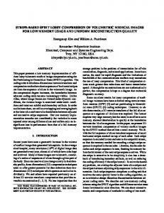
quantization of transformed coefficients is magnified by the inverse procedure of the histogram packing in a decoder. As a result, high quality of reconstructed images can’t be obtained. On the contrary, when a lossy JPEG-LS in near lossless mode is utilized, its rate control is limited to coarse and high PSNR at high bit rate can't be realized. This is because the prediction based near lossless coding has a constrain that the quantization step size must be an integer. In this paper, to attain both of high image quality and fine rate control, we introduce a ‘lossy’ mapping and combine it with a ‘lossless’ coding. In our method, any kind of coding algorithms such as JPEG 2000 based on an integer transform, and JPEG LS based on a prediction can be used as a lossy coding. As a lossy mapping, the local packing of histogram introduced in [6] can be a candidate as a rate optimized method. However it is not always optimum in the ratedistortion sense. The Lloyd-Max quantization in [7] can be another candidate. However both of them are not adaptive to the histogram sparseness, and also they require heavy computational load to find the optimum solution. Unlike these methods, a lossy mapping used in this paper is quite simple to implement without degrading rate distortion performance of the Lloyd-Max quantization. In our experiments, we confirm that the proposed method attains higher performance in the rate-distortion plane than the existing methods. This is because it can utilize histogram sparseness of images, and also its inverse mapping does not magnify quantization noise. 2. EXISTING METHOD A sparse histogram image discussed in this paper is defined. Existing methods and their problems are described. 2.1. Sparse Histogram Image Fig.1(a) illustrates a histogram of a standard image ‘Lena’. Intensity of a pixel value x(n1,n2) at vertical location n1 and horizontal location n2 is represented with an 8 bit integer. This image does not use all the available 28 slots. Defining the histogram sparseness by
| {x | Pr( x) 0} | 100 max{x} min{x} 1
(1)
it has α=95.2 [%] sparseness. In the equation, |X| denotes the cardinal number of a set X. In this case, it means the number of non-zero histogram bins. When we apply
x' (n1 , n2 ) HstEq Floor x(n1, n2 ) /
(2)
to this image, its sparseness becomes α=53.5 [%] for β=1.8. In the equation, ‘Floor[p]’ means the largest integer not greater than p, and ‘HstEq’ means histogram equalization (We used ‘histeq’ function in MATLAB). This is an example of the ‘sparse histogram image’. In HDR representation, an image tends to be sparse in this sense due to its huge number of histogram bins. It often occurs by an image pre-processing such as a histogram modification, a tone mapping, a Gamma correction, an extraction of a region of interest, and so on. In this paper, we consider the histogram sparse image like this.
M T x Lossless y Lossless input Mapping Coding
data
Fig.2 ‘Lossless’ encoding for sparse histogram images. M x Lossless y input Mapping
T e Lossy Coding
data
(a) type I
input
input
x
x
L e'' T Lossy y Lossless Mapping Coding
data
(b) type II (proposed) T e Lossy Coding
data
(c) type III (existing) probability
probability
0.025 0.01 0.005 0
0
50
100
150
200
0.01
2.3. Lossy Mapping and Lossless Coding
0.005 0
250
Fig.3 ‘Lossy’ encoding for sparse histogram images.
0.02 0.015
0
50
100
0.025
dense
0.01 0.005 0
0
20
40
pixel value
(a) α=95.2, β=1
150
200
250
pixel value
probability
probability
pixel value
60
sparse
0.02 0.015 0.01 0.005 0
0
20
40
60
pixel value
(b) α=53.5, β=1.8
Fig.1 Histogram of an image ‘Lena’.
Our purpose is to construct a ‘lossy’ coding for histogram sparse images. A direct expansion is a simple combination of a lossless mapping and a lossy coding as illustrated in Fig.3(a). When a transform is used in the lossy coding like JPEG 2000, quantization noise generated inside the lossy coding is magnified by the inverse mapping. It degrades reconstructed image quality. This case is detailed as below. A mapped signal y(n) is transformed by T , and quantized with a step size qm as
1 w(m) Round T y (n) qm
T
2.2. Lossless Mapping and Lossless Coding The histogram packing introduced in [3] converts the sparse histogram into dense one. It maps a sparse set of original values x into a dense set of values y as y ( n) M x ( n), n [n1 , n 2 ]
(3)
where M denotes a mapping as an operation which holds xˆ ( n) x ( n) 0 1 xˆ ( n) M M x ( n) .
(4)
Even though this lossless mapping does not reduce the 1st order entropy itself, it does reduce data volume of sparse images when it is combined with a lossless coding as illustrated in Fig.2 [4,5]. However it has been limited to ‘lossless’, and therefore the bit rate can't be controlled.
1 y (n) qm
e(m)
.
(5)
where ‘Round [p]’ means rounding to the integer nearest to p. It is reconstructed by y ( n) T 1 w( m) qm (6) T 1 T y ( n) e( m) qm where e(m) denotes the quantization noise in transform domain. As a result, we have the reconstructed signal as
xˆ (n) M 1 T 1 T M x(n) e(m) qm x(n) M
1
T
1
e(m) qm .
(7)
This means that the probability density function of the quantization noise e(m) in transform domain is scattered by the inverse transform T -1 .
Similarly, when a near lossless prediction is used like JPEG LS, we have a reconstructed image as
xˆ (n) x(n) M 1 e' (n) qm
(8)
where e'(n) denotes the quantization noise in spatial domain. In both cases, the error is magnified by the inverse mapping M -1 . Therefore high quality reconstructed images can’t be obtained.
Therefore, unify s+1 bins into one for Nh(s+1) non-zero bins of H(x), and unify s bins into one for (L-Nh)s non-zero bins. This simple procedure fully utilizes the histogram sparseness of input images. Step 3. Calculate the tables Q and R in (11) as below. It unifies s+1 bins for the first Nh classes, and unifies s bins for the rest L-Nh classes as an example. Q(mi )
3. PROPOSED METHOD A new lossy coding for sparse histogram image is described. It can utilize the histogram sparseness of images, and its mapping does not magnify the quantization noise. 3.1. Lossy Mapping and Lossless Coding Fig.3(b) illustrates our coding scheme. We utilize a lossy mapping, and combine it with a lossless coding. In this case, we have the reconstructed signal as xˆ (n) L T T L x(n) x(n) e' ' (n) 1
1
(9)
(10)
and L denotes a lossy mapping. Note that the noise e''(n) is generated in spatial domain by the mapping, and therefore the noise is not magnified by the inverse mapping. 3.2. Weighted Median Cut Quantization (WMCQ) Procedure of the lossy mapping is detailed as below. Due to similarity to the median cut quantization, we refer to it as ‘weighted median cut quantization (WMCQ)’. It reduces 2N kinds of tones for a pixel value x to L tones (2N >L), and it can utilize ‘sparseness’ of the histogram H(x). Forward mapping and backward mapping are performed with tables Q and R as y (n) L x(n) Qx(n) (11) xˆ (n) L1 y (n) R y (n) and therefore these tables should be prepared beforehand. Step 1. Calculate a histogram H(x) of integer pixel values x [0, 2N ). Note that not all the 2N bins but only Ne bins have non-zero values for a sparse image where Ne