Task-Oriented Lossy Compression of Magnetic ... - CiteSeerX

Task-Oriented Lossy Compression of Magnetic Resonance Images by Mark Charles Anderson B.Sc. (Comp. Sci.) University of British Columbia 1990

a Thesis submitted in partial fulfillment of the requirements for the degree of Master of Science

in the School of Computing Science

c Mark Charles Anderson 1995

SIMON FRASER UNIVERSITY July 1995

All rights reserved. This work may not be reproduced in whole or in part, by photocopy or other means, without the permission of the author.

APPROVAL Name: Degree: Title of Thesis:

Mark Charles Anderson Master of Science Task-Oriented Lossy Compression of Magnetic Resonance Images

Examining Committee: Dr. Lou Hafer Chair

Dr. M. Stella Atkins Senior Supervisor Dr. Jacques Vaisey Supervisor Dr. Ze-Nian Li Examiner

Date Approved: ii

Abstract Magnetic resonance tomography produces large quantities of three-dimensional medical image data. Data compression techniques can be used to improve the eciency with which these images can be stored and transmitted, but in order to achieve signi cant compression gains, lossy compression techniques (which introduce distortion into the images) must be used. Conventional metrics of distortion do not measure the eect of this \loss" on tasks applied to the images. This thesis uses a new task-oriented image quality metric which measures the similarity between a radiologist's manual segmentation of brain lesions in raw (not compressed) magnetic resonance images and automated segmentations performed on raw and compressed images. To compress the images, a general wavelet-based lossy image compression technique, embedded zerotree coding, is used. A new compression system is designed and implemented which enhances the performance of the zerotree coder by using information about the location of important anatomical regions in the images, which are coded at dierent rates. Application of the new system to magnetic resonance images is shown to produce compression results superior to the conventional methods, with respect to the segmentation similarity metric.

iii

Acknowledgements I would like to thank my senior supervisor, Dr. Stella Atkins, for her invaluable guidance and enthusiasm throughout the course of this work. I am also grateful to Dr. Jacques Vaisey for his help with the theory and practice of data compression and signal processing. Thanks also to Dr. Ze-Nian Li for taking the time to act as thesis examiner, and to Dr. Lou Hafer for chairing the examining committee. I would also like to thank Blair Mackiewich, for his helpful suggestions and discussions, and Brian Johnston, author of the MRI segmentation algorithm. I am grateful to Don Paty, Andrew Riddehough, Keith Cover, Brenda Rhodes, and Torre Zuk of the University of British Columbia MS/MRI Study Group for supplying the data used in this research. The software used in this work was implemented using the WiT visual programming environment, provided by Terry Arden of Logical Vision Ltd. I am also grateful to Bob Lewis at UBC Imager Lab, author of the wvlt library, for his help with wavelet lters. This research was supported in part by the Natural Sciences and Engineering Research Council of Canada and by Simon Fraser University.

iv

Contents Abstract . . . . . . . . . . . . . . . . . . . . . . . . . . . . . . . . Acknowledgements . . . . . . . . . . . . . . . . . . . . . . . . . . List of Tables . . . . . . . . . . . . . . . . . . . . . . . . . . . . . List of Figures . . . . . . . . . . . . . . . . . . . . . . . . . . . . 1 Introduction . . . . . . . . . . . . . . . . . . . . . . . . . . . 1.1 Motivation . . . . . . . . . . . . . . . . . . . . . . . 1.2 Background . . . . . . . . . . . . . . . . . . . . . . . 1.2.1 Magnetic Resonance Imaging . . . . . . . . 1.2.2 Segmentation of Multiple Sclerosis Lesions 1.3 Research Methodology . . . . . . . . . . . . . . . . . 1.3.1 Methods . . . . . . . . . . . . . . . . . . . 1.3.2 Implementation . . . . . . . . . . . . . . . 1.4 Outline of the Thesis . . . . . . . . . . . . . . . . . . 2 Digital Image Compression . . . . . . . . . . . . . . . . . . 2.1 Data Compression . . . . . . . . . . . . . . . . . . . 2.2 Image Compression . . . . . . . . . . . . . . . . . . . 2.3 Lossless Image Compression . . . . . . . . . . . . . . 2.4 Distortion and Quality . . . . . . . . . . . . . . . . . 2.5 Progressive Techniques . . . . . . . . . . . . . . . . . 2.6 Lossy Compression Techniques . . . . . . . . . . . . 2.6.1 Transform Coding . . . . . . . . . . . . . . 2.6.2 Blocking Transforms and JPEG . . . . . . 2.6.3 Vector Quantization . . . . . . . . . . . . . 3 Wavelets and Zerotree Coding . . . . . . . . . . . . . . . . . v

. . . . . . . . . . . . . . . . . . . . . . . .

. . . . . . . . . . . . . . . . . . . . . . . .

. . . . . . . . . . . . . . . . . . . . . . . .

. . . . . . . . . . . . . . . . . . . . . . . .

. . . . . . . . . . . . . . . . . . . . . . . .

. . . . . . . . . . . . . . . . . . . . . . . .

. . . . . . . . . . . . . . . . . . . . . . . .

. . . . . . . . . . . . . . . . . . . . . . . .

. . . . . . . . . . . . . . . . . . . . . . . .

. . . . . . . . . . . . . . . . . . . . . . . .

iii iv viii ix 1 1 3 3 3 5 5 8 8 10 10 11 12 12 14 16 16 17 19 21

3.1 3.2

4

5

6

Subband Coding . . . . . . . . . . . . . . . . . . . . . . The Wavelet Transform . . . . . . . . . . . . . . . . . . 3.2.1 Background . . . . . . . . . . . . . . . . . . . . 3.2.2 Implementation . . . . . . . . . . . . . . . . . 3.2.3 One-Dimensional Transform . . . . . . . . . . 3.2.4 Two-Dimensional Transform . . . . . . . . . . 3.3 Image Compression using Wavelets . . . . . . . . . . . . 3.4 Embedded Zerotree Coding . . . . . . . . . . . . . . . . 3.4.1 Zerotrees . . . . . . . . . . . . . . . . . . . . . 3.4.2 Implementation . . . . . . . . . . . . . . . . . 3.4.3 Performance . . . . . . . . . . . . . . . . . . . Task-Oriented Compression . . . . . . . . . . . . . . . . . . . . 4.1 Semi-Automatic Lesion Segmentation . . . . . . . . . . 4.2 Baseline Results . . . . . . . . . . . . . . . . . . . . . . 4.2.1 Segmentation of the Raw Data . . . . . . . . . 4.2.2 Segmentation of the Compressed Data . . . . . 4.3 Adaptation . . . . . . . . . . . . . . . . . . . . . . . . . 4.3.1 Inter-Slice Correlation . . . . . . . . . . . . . . 4.3.2 Multispectral Compression . . . . . . . . . . . 4.3.3 Band-Speci c Thresholds in EZW . . . . . . . Region-Based Compression . . . . . . . . . . . . . . . . . . . . 5.1 Region-Based Coding . . . . . . . . . . . . . . . . . . . 5.1.1 Image Partition . . . . . . . . . . . . . . . . . 5.1.2 Spatial-Domain Partition . . . . . . . . . . . . 5.1.3 Transform-Domain Partition . . . . . . . . . . 5.1.4 Region Bit Rate and PSNR . . . . . . . . . . . 5.2 Volume Bit Rate Allocation . . . . . . . . . . . . . . . . 5.3 Implementation . . . . . . . . . . . . . . . . . . . . . . . 5.3.1 Spatial Region-Based EZW0 (SRB-EZW0 ) . . . 5.3.2 Transform Region-Based EZW0 (TRB-EZW0 ) . 5.3.3 Overheads . . . . . . . . . . . . . . . . . . . . Experimental Results . . . . . . . . . . . . . . . . . . . . . . . . 6.1 Single Slice Coding . . . . . . . . . . . . . . . . . . . . . vi

. . . . . . . . . . . . . . . . . . . . . . . . . . . . . . . . .

. . . . . . . . . . . . . . . . . . . . . . . . . . . . . . . . .

. . . . . . . . . . . . . . . . . . . . . . . . . . . . . . . . .

. . . . . . . . . . . . . . . . . . . . . . . . . . . . . . . . .

. . . . . . . . . . . . . . . . . . . . . . . . . . . . . . . . .

. . . . . . . . . . . . . . . . . . . . . . . . . . . . . . . . .

. . . . . . . . . . . . . . . . . . . . . . . . . . . . . . . . .

. . . . . . . . . . . . . . . . . . . . . . . . . . . . . . . . .

21 21 22 22 24 26 28 29 29 31 36 40 40 42 42 43 48 48 49 49 52 52 52 54 56 56 58 59 60 60 63 64 64

6.2 Volume Coding and Segmentation Similarity 6.3 Progressive Transmission . . . . . . . . . . . 7 Summary and Conclusions . . . . . . . . . . . . . . . 7.1 Review . . . . . . . . . . . . . . . . . . . . . 7.2 Future Work . . . . . . . . . . . . . . . . . . Bibliography . . . . . . . . . . . . . . . . . . . . . . . . .

vii

. . . . . .

. . . . . .

. . . . . .

. . . . . .

. . . . . .

. . . . . .

. . . . . .

. . . . . .

. . . . . .

. . . . . .

. . . . . .

. . . . . .

. . . . . .

. . . . . .

69 79 82 82 83 85

List of Tables 3.1 3.2 3.3 3.4

The wavelet2d operator. . . . . . . . . . . . . . . . . . . The ztcompress operator. . . . . . . . . . . . . . . . . . . The ztexpand operator. . . . . . . . . . . . . . . . . . . . EZW coding results for \Lena" and \Barbara" images. .

. . . .

. . . .

. . . .

. . . .

. . . .

. . . .

. . . .

. . . .

. . . .

. . . .

. . . .

. . . .

32 32 32 36

4.1 Volume similarity indices for lesion segmentations, raw and compressed. . . . 46 5.1 The wmask operator. . . . . . . . . . . . . . . . . . . . . . . . . . . . . . . . . 62 6.1 Interor and exterior bit rates used to code a single slice. . . . . . . . . . . . . 67 6.2 PSNR of brain region of EZW0 reconstructions. . . . . . . . . . . . . . . . . . 69 6.3 Volume similarity indices for lesion segmentations, raw and compressed . . . 78

viii

List of Figures 1.1 1.2 1.3 1.4

Sample MRI volume. . . . . . . . . . MR image slices. . . . . . . . . . . . ROIs isolating MS lesions in slice 17. Example of a WiT igraph. . . . . . .

. . . .

. . . .

. . . .

. . . .

. . . .

. . . .

. . . .

. . . .

. . . .

. . . .

. . . .

. . . .

. . . .

. . . .

. . . .

. . . .

. . . .

. . . .

. . . .

. . . .

. . . .

. . . .

. . . .

4 6 7 8

2.1 Data compression. . . . . . . . . . . . . . . . . . . . . . . . . . . . . . . . . . 10 2.2 Progressive image reconstruction. . . . . . . . . . . . . . . . . . . . . . . . . . 15 2.3 Reconstructions of a JPEG-coded image. . . . . . . . . . . . . . . . . . . . . . 18 3.1 3.2 3.3 3.4 3.5 3.6 3.7 3.8 3.9 3.10 3.11 3.12 3.13

Block diagram of wavelet analysis and synthesis. . . . . . . . . Block diagram of two-level pyramidal analysis system. . . . . . Application of the 1-dimensional wavelet transform. . . . . . . Subbands in the hierarchical 2-dimensional wavelet transform. . Application of the 2-dimensional wavelet transform. . . . . . . Histograms of an image and its wavelet transform. . . . . . . . Reconstruction of a wavelet-transformed image. . . . . . . . . . WiT hierarchical operators used for EZW0 compression . . . . . WiT igraph to compress an image using EZW0 . . . . . . . . . . WiT igraph to decompress an image using EZW0 . . . . . . . . . EZW0 reconstructions of \Lena" and \Barbara" images. . . . . Reconstructions of an EZW0 -coded MR image. . . . . . . . . . PSNR of JPEG and EZW0 reconstructions. . . . . . . . . . . .

. . . . . . . . . . . . .

. . . . . . . . . . . . .

. . . . . . . . . . . . .

. . . . . . . . . . . . .

. . . . . . . . . . . . .

. . . . . . . . . . . . .

. . . . . . . . . . . . .

. . . . . . . . . . . . .

23 23 25 26 27 28 29 34 35 35 37 38 39

4.1 Binary lesion segmentations. . . . . . . . . . . . . . . . . . . . . . . . . . . . . 42 4.2 Similarity indices for each slice of the segmentation. . . . . . . . . . . . . . . 43 4.3 PSNR of EZW0 compressed slices. . . . . . . . . . . . . . . . . . . . . . . . . 44 ix

4.4 Semi-automatic segmentation of compressed data. . . . . . . . . . . . . . . . 45 4.5 Similarity indices of EZW0 and JPEG compressed slices. . . . . . . . . . . . . 47 4.6 Results of using band-speci c thresholds in EZW0 . . . . . . . . . . . . . . . . 51 5.1 5.2 5.3 5.4 5.5 5.6 5.7

Sample MRI volume brain mask. . . . . . . . . . . . . . . . . . . Subimage partition in the spatial domain. . . . . . . . . . . . . . Subimage partition in the transform domain. . . . . . . . . . . . WiT igraph to code a single slice using SRB-EZW0 . . . . . . . . . WiT igraph to reconstruct a single slice coded with SRB-EZW0 . . WiT igraph to code a single slice using TRB-EZW0 . . . . . . . . WiT igraph to reconstruct a single slice coded with TRB-EZW0.

. . . . . . .

. . . . . . .

. . . . . . .

. . . . . . .

. . . . . . .

53 55 57 60 61 61 62

6.1 6.2 6.3 6.4 6.5 6.6 6.7 6.8 6.9 6.10 6.11 6.12 6.13 6.14 6.15

Results of SRB-EZW0 coding of single slice. . . . . . . . . . . . . . . . Results of TRB-EZW0 coding of single slice. . . . . . . . . . . . . . . . Pro le plot of SRB-EZW0 reconstruction, showing mask edge artifact. Brain region PSNR of each slice of the PD-weighted reconstructions. . Slices from 0.25 bpp SRB-EZW0 reconstruction. . . . . . . . . . . . . . Size of the brain mask in pixels for each slice. . . . . . . . . . . . . . . Interior and exterior bit rates yielding an overall bit rate of 0.25 bpp. . Slices from 0.25 bpp TRB-EZW0 reconstruction, p = 0:9. . . . . . . . . Reconstructed slices using TRB-EZW0 with p = 0:7. . . . . . . . . . . Manual and automatic segmentations of the raw data. . . . . . . . . . Automatic segmentation of SRB-EZW0 compressed images. . . . . . . Automatic segmentation of TRB-EZW0 compressed images. . . . . . . Slice similarity indices for SRB-EZW0 , p = 1:0. . . . . . . . . . . . . . Slice similarity indices for TRB-EZW0 , p = 0:9 and p = 0:7. . . . . . . Progressive image reconstruction using TRB-EZW0 . . . . . . . . . . .

. . . . . . . . . . . . . . .

. . . . . . . . . . . . . . .

. . . . . . . . . . . . . . .

. . . . . . . . . . . . . . .

65 66 68 70 71 72 72 73 74 75 76 77 79 80 81

x

. . . . . . .

. . . . . . .

Chapter 1

Introduction 1.1 Motivation Traditionally, medical images such as radiographs were generated and stored on lm, but many advanced medical imaging modalities such as computed tomography (CT) and magnetic resonance imaging (MRI) collect the data digitally. Thus, the amount of data stored in digital form is increasing. The images use vast amounts of storage space, and may require long transmission times when sent over communication lines to remote locations, such as in teleradiology [55]. Compression techniques have long been used to alleviate the storage and transmission problems for large data les. For image data, compression techniques fall into two categories. Lossless, or reversible, compression of digital images preserves all of the information in the original image. Lossy, or irreversible, compression can achieve more compression by storing or transmitting an approximation of the original image, so that the reconstructed image contains some noise or distortion. Such distortion may consist of both the removal of detail from the original image, and the introduction of artifacts that were not present in the original image. The additional compression that can be achieved using lossy techniques is usually justi able for image data because the human visual system can tolerate error in the restored output. However, such lossy compression techniques have not been conclusively adopted in the medical imaging community due to the perceived or actual distortion of clinically signi cant image detail. In a medical imaging environment, vast quantities of data are generated, transmitted, and stored. For instance, a typical hospital might generate on the order of 1000 gigabytes 1

CHAPTER 1. INTRODUCTION

2

of image data per year [55]. Even a single MRI volume of 1.5 megabytes (MB) might take half an hour to transmit over a telephone line operating at 9600 bits per second (bps). Thus, to achieve practical storage and transmission times, compression ratios of at least 10:1 are desired, while 20:1 or 30:1 compression would be preferable. In our MRI example, the transmission time would be reduced to one minute if a compression of 30:1 could be achieved. The amount of compression that can be achieved using lossless methods may be inadequate for the large quantities of data generated in a medical imaging environment [16, 18, 37, 39, 55]. However, even if lossy compression has not yet been accepted for use in diagnostic medical imaging, it may be bene cial to employ lossy compression techniques for other purposes. For example, the original image may be used for diagnosis, but the image can be compressed using a lossy method for archival storage. Similarly, when a large image is being retrieved from storage or transmitted to a remote location, it may be bene cial to rst transmit a lower-quality approximation for initial examination, followed by the slower transmission of further detail required for closer scrutiny.1 Indeed, the recent increased interest in the use of lossy compression techniques for medical image compression is re ected in the proposed standard for Digital Imaging and Communications in Medicine (DICOM) [47]. When lossy compression is used, it is desirable to preserve as much clinically useful information as possible. The nature of the information to be retained and to be discarded depends on both the type of image and the diagnostic task to be performed. One goal of this research is to determine the eects of lossy compression on certain medical imaging applications. There exist a number of objective measures of reconstructed image quality and distortion, but the relationship of these measures to the actual performance of applications on the reconstructed images has not been clearly identi ed. This thesis provides a new system for the lossy compression of medical images that takes advantage of certain known characteristics of the data and of the applications that will be applied to the data, with the goal of improving compression performance while maintaining the eectiveness of the applied medical imaging tasks. In this thesis, the applications of information storage and retrieval are considered to be equivalent to transmission and reception respectively. 1


3

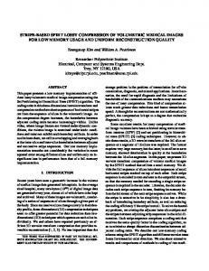
1.2 Background 1.2.1 Magnetic Resonance Imaging In computerized tomographic imaging, multiple cross-sectional images are obtained through the body to produce a 3-dimensional volume image. Magnetic resonance imaging (MRI) is a form of computerized tomographic imaging in which data is acquired by measuring the interaction between pulses of radio frequency (RF) radiation and tissues in a strong magnetic eld. These data are then transformed to reconstruct a 3-dimensional digital image volume. Figure 1.1 depicts the 27 slices comprising an example MR volume. In MRI, several tissue characteristics can be measured, including the proton density (PD), the longitudinal relaxation time (T1), and the transversal relaxation time (T2). The magnitude or intensity of each voxel of an MR volume image is related to the PD, T1, and T2 of the tissues located at the corresponding anatomical position; dierent tissues appear with dierent characteristic intensities. The contrast between dierent tissue types can be controlled at the time of acquisition by varying several MRI parameters including the pulse repetition time (TR) and echo time (TE ). Choice of these parameters can result in PD-weighted, T1 -weighted, or T2-weighted images. Since multiple registered images of the same anatomical slice with dierent weightings can be acquired simultaneously, MRI data is inherently multispectral. For more information about magnetic resonance imaging, the reader is encouraged to consult [40, 54]. Because of the excellent contrast and detail resolution which can be achieved, MRI is a particularly good method for visualizing anatomical features and pathologies. It is often used to obtain images of the the Central Nervous System (CNS), which consists of the brain and spinal cord. The CNS tissues are of two types: the white matter and the gray matter. White matter bres conduct the nerve impulses and are electrically insulated by a fatty substance, myelin.

1.2.2 Segmentation of Multiple Sclerosis Lesions In MR images of the brain, the white and gray matter tissues appear with dierent intensities, depending on the acquisition parameters. In PD-weighted scans, the gray matter usually appears brighter and the white matter darker; in T2-weighted scans the reverse is true. The cerebrospinal uid (CSF) and tissues such as muscle, fat, and bone of the skull


Figure 1.1: The 27 slices of the sample MRI volume.

4


5

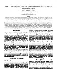
appear with other characteristic intensities. Figure 1.2 shows three slices of an MR volume in both PD and T2 weighted acquisitions. Multiple sclerosis (MS) is a progressive disorder of the CNS whose symptoms include weakness, lack of coordination, abnormal sensations, and speech and visual impairment. The disease is characterized by a breakdown of myelin sheathing in parts of the white matter [21]. The resulting plaques or lesions are visible in MR images as bright patches, usually in the white matter, such as are visible in slice 17 of both the PD and T2 weighted images in Figure 1.2. Both the clinical symptoms of MS and extent of lesions found in the brain tend to change over long periods of time, and the quanti cation of lesion volume plays an important role in the evaluation of drug treatments. Traditionally, the classi cation or segmentation of brain tissues has been performed by radiologists by manually tracing the outlines of tissues on digital images displayed on computer graphics terminals with a pointing device. Each such outline de nes a region of interest (ROI). A set of ROIs isolating MS lesions in slice 17 of the data in Figure 1.2 is displayed in Figure 1.3. The manual segmentation of an MR image set into ROIs of dierent tissue types is a slow and tedious task, and the problem of automatic computerized segmentation has been the focus of considerable research [74].

1.3 Research Methodology 1.3.1 Methods MR images of the brain containing MS lesions were segmented using a semi-automatic technique. As a part of the pre-processing of the image data for segmentation, identi cation of the contour of the brain surface inside the intracranial cavity is required. Recent research has provided an automatic method for detecting this contour in an arbitrary MRI volume [45]. Since the data outside the brain contour is of no use to the segmentation, this provides a means of partitioning the volume into disjoint subimages of diering relative importance, and this information can be used to improve compression. Most image compression systems are general-purpose and can be applied to any kind of image data, though the performance will vary according to the nature of the input data. In this thesis we adapt a general image compression scheme and improve its performance on a particular class of images. After considering various image compression techniques, we used wavelet-transform


6

(a)

(b)

(c)

(d)

(e)

(f)

Figure 1.2: MR image slices, PD-weighted (left) and T2-weighted (right). Slices 1 (top), 17 (middle), and 27 (bottom).


7

Figure 1.3: ROIs isolating MS lesions in slice 17. based subband coding, which, in addition to being very suitable for general image compression tasks, can be used to take advantage spatial as well as frequency information in the input image, and is therefore well-suited to our region-based approach. A state-of-the-art still-image compression method, embedded zerotree wavelet (EZW) coding, oers superior rate-distortion performance, ne bit-rate control, and progressive coding. We implemented an EZW coder and decoder using a visual programming language (described below). The MR images were compressed using EZW and reconstructed at various bit rates, and the semi-automatic segmentation was performed. Then, as a new approach to measuring the quality of the compression, we used a numerical similarity measure to compare the results of the semi-automatic MS lesion segmentation with the radiologist's gold-standard segmentation. Our EZW implementation was adapted to take advantage of the spatial information provided by the brain contour. By specifying which portions of the input image are more important, the new technique splits the data into two subimages which are coded at dierent rates. The variation in area of the brain contour along the z -axis of the volume is also used

CHAPTER 1. INTRODUCTION rdObj

8 lopass2d

display

original

filename: image.wit

width: 3 height: 3

name: blurred

Figure 1.4: Example of a WiT igraph. to control the allocation of bits when compressing each slice. This new method is used to compress the same MR volume at the same bit rates. The segmentation is performed again, and the similarity measures are calculated and compared to results on original data and the data compressed using conventional methods.

1.3.2 Implementation The image processing tasks performed in the course of this research were implemented in the WiT TM visual programming language [4, 5]. WiT programs, or igraphs, consist of operators connected by links. Data objects ow on the links from operator to operator. Operators perform functions on the input data objects and produce output data objects. Libraries of standard image-processing and other operators are provided as a part of WiT, and custom operators and data objects can be created by the user. An operator may itself be de ned by a WiT igraph with input and output links; such an operator is called hierarchical, and can be used like any other operator in igraphs. Hierarchical operators are analogous to subroutines in a conventional programming language. Operators may also be coded in C. Figure 1.4 shows an igraph with three operators, shown as rectangular icons, connected from left to right with links. Each operator's name is displayed above its icon; its parameters and their values are shown below. In this igraph the rdObj operator reads an image from disk, lopass2d applies a low-pass lter using a 3 3 kernel, and display displays the resulting image in a window. A probe labelled original causes the raw image to be displayed as it passes along the rst link.

1.4 Outline of the Thesis In Chapter 2, techniques for digital image compression are discussed. Previous work in the compression of medical images is surveyed.


9

Chapter 3 describes the wavelet transform and its application to image compression, focussing on the EZW algorithm. Chapter 4 discusses some approaches to the adaptation of compression techniques for certain classes of medical image data and tasks, in particular for the segmentation of whitematter brain lesions in magnetic resonance volume data. A quality measure based on the similarity between such image segmentations is de ned, and results for images compressed using conventional EZW are presented. In Chapter 5, a new region-based adaptation of EZW is presented. In Chapter 6, experimental results of the region-based EZW method are given. In Chapter 7, the research is summarized and potential directions for future research are considered.

Chapter 2

Digital Image Compression Digital image compression has been the focus of a large amount of research in recent years [23, 32, 52]. This chapter reviews image compression algorithms with particular focus on the compression of medical images.

2.1 Data Compression Compression techniques take advantage of the redundant and irrelevant information contained in the data [52]. Redundancy results from the statistical correlation of data elements, while irrelevancy concerns the uselessness of some of the information contained in the data. In general, compression schemes consist of three steps, as depicted in Figure 2.1, where decorrelation is the application of some transformation or decomposition to reduce the statistical redundancy of the input data; quantization is the many-to-one mapping of input values onto a smaller set of output symbols; and coding is the ecient representation (entropy coding) of the quantized values as a bit stream. samples

?! decorrelation

coecients ?!

?! ecient coding lossy quantization symbols

Figure 2.1: Data compression. 10

bit?! stream

CHAPTER 2. DIGITAL IMAGE COMPRESSION

11

Lossless techniques omit the quantization step, since it is inherently lossy. However, it is also the step in which the majority of the data compression can be realized. The process of decompression consists of the same steps executed in reverse order. Compression of text sources generally employs only entropy coding. Human coding [29] employs a variable length code in which short code words are assigned to more common values or symbols in the data, and longer codes are assigned to less frequently occurring values. Lempel-Ziv (LZ) coding [69] replaces repeated substrings in the input data with references to earlier instances of the strings. Variations of LZ coding are used by the Unix compress and gzip programs. Arithmetic coding [70, 50] represents a message as some nite interval between 0 and 1 on the real number line. Each bit in the output code re nes the precision of the value of the input code in the interval. The entropy coder used in this work is an adaptive arithmetic coder, which is preferable to Human coding at low bit rates because Human coding requires at least one bit per code symbol to be emitted, while arithmetic coding does not.

2.2 Image Compression In image compression, entropy coding is generally preceded by decorrelation (to reduce redundancy in the image data) and, for lossy compression, quantization. In two-dimensional image coding, redundancy refers to the correlation among nearby pixels in a single image, but such correlation may exist among pixels in multidimensional data such as in a volume image, time series, video sequence, or in dierent spectral bands in a multispectral data set [25]. The eectiveness of an image compression technique is measured by the amount of compression achieved and, for lossy techniques, the quality of the reconstructed image. We must take some care when reading claims of the amount of compression obtained. One frequently used measure is compression ratio, or the ratio of the size of the original image to the size of the compressed image. This measure can be misleading, since it is dependent on the data storage format and sampling density. For example, medical images containing 12 bits of useful information per pixel are often stored using 16 bits per pixel. A better measure of compression is bit rate, which measures the average number of bits used to represent each pixel of the image in compressed form (and is thus independent of the data storage format).


12

If an n m pixel image is stored using B bits, the bit rate is

B R = nm

Bit rates are measured in bits per pixel (bpp), with a lower bit rate corresponding to a greater amount of compression. In discussing claims of compression eciency reported in the literature, we quote the bit rate where it is given (or where it is possible to calculate); otherwise the compression ratio alone is given.

2.3 Lossless Image Compression Lossless entropy-coding techniques for data compression can be applied directly to image data. For instance, the popular GIF image format uses an LZ coder for its lossless compression. Typically, medical images can be compressed losslessly to about 50 per cent of their original size. Boncelet et al. [10] investigated the use of three entropy coding methods for lossless compression with application to digitized radiographs and found that a bit rate of about 4 to 5 bpp was the best possible. The Human and arithmetic coders performed about equally well. Tavakoli [65, 66] applied various lossless coding techniques to MR images and reported compression down to about 5 to 6 bpp, with LZ coding giving the best results. Lossless coders work best with decorrelated data. Roos et al. [58, 57] investigated methods for decorrelating image data before coding medical images. These techniques, which include prediction, linear transformation, and multiresolution methods, are described in greater detail in section 2.6. Angiograms could be compressed with a ratio of up to 3:1, but results were less than 2:1 for MRI, which contain more noise. Kuduvalli and Rangayyan [38] studied similar techniques and found linear prediction and interpolation techniques gave the best results, with similar compression ratios. We conclude that lossless coding cannot achieve the higher compression ratios which we have established as desirable for eective archiving and transmission of medical images.

2.4 Distortion and Quality Signi cant coding gains can be achieved by sacri cing the ability to perfectly reconstruct the original image, and lossy image compression methods trade o the quality of the reconstructed image against the bit rate that can be attained. The \quality" of the reconstruction


13

is a measure of how close it is, in some sense, to the original image. There are many practical measures of image quality [18], including:

subjective comparison: how \good" the image looks to a human viewer application quality: usefulness of the image for a particular task, e.g. clinical diagnosis (for medical images)

mean square error (MSE) signal-to-noise ratio (SNR) When comparing two lossy coding methods, we may either compare qualities of images reconstructed at a constant bit rate, or, equivalently, we may compare the bit rates used in two reconstructions with the same quality, if it is possible to establish this. Ideally, when comparing the eects of lossy coding algorithms, we would like to use an objective method. Objective measures such as the SNR and MSE of the reconstructed image are easy to compute but they do not adequately characterize the distortion present in the image [18]. For instance, artifacts that are particularly objectionable to the human viewer may not be re ected by poor numerical SNR or MSE. There has been some research into the quanti cation of the artifacts introduced by various lossy compression schemes. For instance, Ho et al. [26] de ned a measure of the \blockiness" introduced into images compressed using certain algorithms, but such a measure cannot be used to compare compression algorithms in general. The diagnostic quality of a medical image may remain high even when its subjective quality is signi cantly degraded [15]; this depends on the characteristics of the pathological features in the image and the clinical task being performed. Receiver Operating Characteristic (ROC) methods are frequently used to obtain and evaluate a \gold standard" in the medical imaging community [16, 18]; expert viewers are asked to assess a degree of con dence in the presence or absence of diagnostic features in the images. However, these and other subjective measurements suer from their dependence on human judgement; they are time-consuming to perform, and their results may be dicult to reproduce. Because of these diculties, the subjective visual appearance of images is considered only informally in this thesis. The peak signal-to-noise ratio (PSNR) is an objective quality measure often used in image compression literature, and so we will use it for purposes of


14

comparison. Consider an original image f and a distorted version of the image, f^, both of size m n pixels. The mean-square error (MSE) 2 in f^ with respect to f is de ned by 1 2 = mn

?1 mX ?1 nX i=0 j =0

(f^i;j ? fi;j )2

(2.1)

and can be interpreted as the squared average dierence between corresponding pixels in the two images. The PSNR is a related measure de ned by 2

PSNR = 10 log10 fmax 2

(2.2)

where fmax is the maximum pixel value (e.g., 255 for 8-bit images). PSNR is expressed in decibels (dB) with larger values indicating better image quality. In this research we will also use a new objective measure of image quality, based on the similarity between results of an image segmentation task on compressed images and the segmentation of the original data.

2.5 Progressive Techniques While lossless coding is preferred for medical imaging, we have seen that the compression gains may not be sucient. For certain applications such as teleradiology, progressive techniques may oer a compromise. As mentioned above, there exists an inverse relationship between coding bit rate and distortion when using lossy compression. Therefore, each additional bit of information used in the reconstruction of an image could, ideally, improve the quality of the image. An image compression method can be called progressive if it allows an image to be gradually built up as more and more bits are received. Initially a low-quality image is reconstructed, and it is then re ned as the information contained in subsequent bits is added. For instance, consider a simple progressive transmission scheme in which the image resolution is gradually increased in steps from 8 8 pixels in the initial approximation (where each pixel represents the average of a 32 32 block of pixels in the source image) up to the original 256 256. The resolution is increased by a factor 2 in both directions in each successive image, and thus each requires 4 times as many bits as the previous. This technique is illustrated in Figure 2.2, where the image sizes have been normalized. Many image compression algorithms allow for more sophisticated progressive reconstruction


15

(a)

(b)

(c)

(d)

(e) (f) Figure 2.2: Illustration of a simple progressive image reconstruction. Image representations using (a) 512 bits, (b) 2048 bits, (c) 8192 bits, (d) 32768 bits, (e) 131072 bits, and (f) the original image containing 524288 bits.


16

techniques. Progressive techniques are particularly well suited to medical imaging applications such as teleradiology [55], where an initial low- delity image transmitted over a low-speed communication link could be used for preliminary consultation, followed by more detailed images required for diagnosis. It is also suitable for browsing image databases, allowing the user to determine quickly whether the selected image is of interest, and thereby to decide to proceed with reconstruction of a higher quality image or abort the retrieval procedure.

2.6 Lossy Compression Techniques 2.6.1 Transform Coding In transform coding, a linear transformation of the data is used to decorrelate it. The data in the transform domain is then quantized, and the quantized transform coecients are entropy-coded. The discrete Karhunen-Loeve transform (KLT) is optimal in its informationpacking properties (in the mean-square error sense) but is hard to compute [32, 23]. The discrete Fourier transform (DFT) and discrete cosine transform (DCT) approximate the energy-packing eciency of the KLT, and have ecient algorithms; in practise, the DCT is almost always used in preference to the DFT because the latter's coecients are complex and thus require twice the storage space of the DCT coecients. Transform coding exploits correlation of the pixels within a rectangular block. Full-frame methods, in which the transform is applied to the whole image as a single block, have been employed in medical imaging research [27, 12, 30]. Bramble et al. [11] used full-frame Fourier transform compression on 12 bpp digitized hand radiographs at average rates from about 0.75 bpp down to 0.1 bpp. The diagnostic task in this study involved the detection of pathology characterized by a lack of sharpness in a bone edge. No signi cant degradation in diagnostic quality was found using images compressed at an average rate of 0.75 bpp, con dence in the diagnoses decreased at rates on the order of 0.5 bpp, and diagnostic quality suered at very low rates of 0.1 bpp. However, Cook et al. [17] investigated the eects of full-frame DCT compression on low-contrast detectability of chest lesions and found signi cant degradation at rates of about 0.75 bpp. These results illustrate that the imaging modality and task play an important role in determining the amount of compression that can be achieved.


17

2.6.2 Blocking Transforms and JPEG In an alternative to full-frame transforms, smaller blocks or tiles covering the image can be used, in what is called a blocking transform; each block is transformed, quantized, and coded separately. This technique, using square 8 8 pixel blocks and the DCT followed by Human or arithmetic coding, is utilized in the ISO Joint Photographic Experts Group (JPEG) Draft International Standard for image compression [31, 49, 3]. The standard recently drawn up by the American College and Radiologists (ACR) and the National Electrical Manufacturers' Association (NEMA) provides for the use of JPEG compression of medical images [47], though it does not address the suitability of compressed images for clinical purposes. While the JPEG standard provides for lossless compression and a progressive mode, only the standard lossy compression has been widely implemented. Lossy JPEG compression uses a numerical \quality" parameter (in the range 1 to 100) to jointly control the amount of compression and the quality of the reconstructed image. It works well at compression ratios up to about 25:1, after which the quality degrades signi cantly due to the presence of blocking artifacts [25]. In addition, such artifacts may become visible at lower compression ratios if the image undergoes certain manipulations, such as contrast adjustment and zooming. Figure 2.3 shows the eects of JPEG image compression of a sample image at various bit rates. At 0.26 bpp (or a compression ratio of 30:1 with respect to an 8 bpp original), the 8 8 pixel blocks are easily visible. At 0.17 bpp (47:1 compression), the image is degraded to such an extent that almost all detail has been lost. Since the adoption of the JPEG standard, the algorithm has been the subject of considerable research. Collins et al. [16] studied the eects of a 10:1 lossy image compression scheme based on JPEG, with modi cations to reduce the blocking artifacts. A number of image types and pathologies were studied using ROC methods, and the preliminary results supported the use of lossy compressed images for comparison purposes such as detecting changes over time. Baskurt et al. [7] used an algorithm similar to JPEG to compress mammograms with rates as low as 0.27 bpp while retaining detectability of pathologies by radiologists. Kostas et al. [37] used JPEG modi ed for use with 12-bit images and custom quantization tables to compress mammograms and chest radiographs. This preliminary work reported compression down to about 0.25 bpp while retaining clinically useful information in varying degrees. Clunie et al. [15] studied the detection of multiple sclerosis lesions in MR images


18

(a)

(b)

(c)

(d)

(e)

Figure 2.3: Reconstruction of a JPEG-coded image. (a) The original image, scaled to 8 bpp. (b) Reconstruction at 1.01 bpp (quality factor 77). (c) Reconstruction at 0.50 bpp (quality factor 35). (d) Reconstruction at 0.26 bpp (quality factor 10). (e) Reconstruction at 0.17 bpp (quality factor 1).


19

of the brain which had been compressed using JPEG, and found no signi cant dierence in the number of lesions detected by radiologists in images compressed at bit rates of 0.3 bpp. However, this study did not evaluate eects of compression on the the size or shape of the lesions.

2.6.3 Vector Quantization Shannon [62] rst showed that quantization of vectors of input codes will result in a lower bit rate than scalar quantization. Gray [24] reviewed various techniques for vector quantization (VQ) of images. In VQ of image data, a vector is a small block of pixels from the original image, and a set of training images is used to generate a codebook of vectors which occur frequently. Each block of input pixels is examined and the index of a vector in the codebook which is \close" (using some measure) to the input vector is emitted. The decoder simply receives each index and looks up the corresponding vector in the codebook. VQ therefore has a very fast decoder|essentially a table lookup|but the coder can be very slow, since it must perform a computationally complex codebook search for each vector. Riskin et al. [55] presented techniques for variable-rate VQ design and applied them to MR images. These techniques somewhat mitigate the complexity problem with the use of more ecient data structures in the codebook to speed up the search. They reported results down to just under 1 bpp. Cosman et al. [18] used similar methods to compress CT and MR chest scans and investigated three quality measures: SNR, subjective quality, and diagnostic accuracy. They found that compression down to about 0.5 bpp did not signi cantly aect a blood-vessel measurement task in MR. Xuan et al. [73] also used similar VQ techniques to compress mammograms and brain MRI. Computerized segmentation of these images without signi cant degradation of the results was possible at rates down to 0.6875 bpp. VQ suers from a lack of generality, since the codebook must be trained on some set of initial images; the bit rate and distortion of the compression will be aected by how representative the training set is of the images to be coded. This restriction can be relaxed using adaptive techniques, in which the codebook is constructed or modi ed during decoding, adapting itself to the data, at the expense of some compression eciency. Hu et al. [28] introduced a semi-adaptive VQ technique for the compression of multispectral MR images, which achieved compression at bit rates down to 0.4 bpp while maintaining diagnostic image quality as judged by radiologists. In addition to the slow coder and codebook requirements mentioned above, images


20

compressed at low bit rates using VQ are prone to artifacts like those resulting from blocking transforms.

Chapter 3

Wavelets and Zerotree Coding 3.1 Subband Coding Subband compression uses a linear transformation to split a signal's frequency component into bands and then codes each band separately [34, 72]. This allows dierent parameters to be used for the transmission of each band, depending on the desired characteristics of the reconstructed image. For instance, the human visual system is more sensitive to distortion in certain frequencies than in others, and so the coding of these bands could be performed more precisely than the others in order to improve the visual quality of the reconstructed image at a given bit rate. Rompelman [56] investigated the use of subband coding for medical image compression and reported that 12-bit CT images could be compressed at rates of 0.75 bpp and 0.625 bpp (16:1 and 19.2:1 respectively) without signi cantly aecting diagnostic quality. Recently, much research has been devoted to the discrete wavelet transform (DWT) for subband coding of images [25]. The wavelet transform is a hierarchical subband decomposition particularly suited to image compression. It avoids the blocking artifacts present in transform methods and allows for easy progressive coding due to its multiresolution nature. For these reasons, we focus on wavelet-based compression in this work.

3.2 The Wavelet Transform In this section we review the Wavelet transform. The reader is referred to [8, 19, 25, 33, 51] for additional details. 21

CHAPTER 3. WAVELETS AND ZEROTREE CODING

22

3.2.1 Background Like other linear transforms, the wavelet transform decomposes an arbitrary signal f into a superposition or weighted sum of some set of basis functions k , as (in one dimension) X f (x) = ck k (x) k

Since the basis functions are xed, the signal f can be represented by the coecients ck alone. The choice of basis function controls the nature of the information about the original signal contained in each coecient. For instance, since sinusoidal functions have in nite support, their use as basis functions will result in a Fourier representation, with coecients having good frequency localization but no spatial localization. By choosing basis functions with nite support of varying widths, the coecients can represent both spatial and frequency information of the input signal at various scales. We can then take advantage of redundancy and irrelevancy in both the spatial and frequency domains for signal compression. Wavelets are functions a;b generated by dilating and translating a single prototype mother wavelet function . x ? b 1 ? a 6= 0 a;b(x) = jaj 2 a

Here a controls the dilation and b the translation of the wavelet. If a and b are powers of 2, an octave-band decomposition is produced, with logarithmic spatial and frequency resolution. The wavelet decomposition of a one-dimensional signal is then X f (x) = ca;b a;b(x) a;b

3.2.2 Implementation The wavelet transform can be implemented using multirate lter banks as shown in the block diagram of Figure 3.1. In this signal-processing framework, the wavelet transform is de ned by the nite impulse response lter pairs H and G. Here analysis is the process whereby the input signal is split into critically-subsampled frequency-related subband signals. In the diagram, lters h0 and h1 split the signal into its low-pass and high-pass components, which are then subsampled and coded. The low-pass or reference signal r is a low-resolution version of the original, while the high-pass or detail signal d contains the detail information which has been removed from the reference signal.


- h0 - # 2 rf (x)

r^- " 2

codec

Analysis

23

- g0 ? - fx 6 +

Synthesis

- h1 - # 2 d-

d^- " 2

codec

^( )

- g1

Figure 3.1: Block diagram of wavelet analysis and synthesis.

f (x)

-

h0

- #2

-

h1

- #2

-

-

h0 h1

- #2 - #2 -

d1

-

d0

r1

Figure 3.2: Block diagram of two-level pyramidal analysis system. The codec represents the coding and decoding of the signals, including the intermediate transmission or storage they may entail. If these processes include quantization, then some distortion will be introduced into the signals, and so the output reference and detail signals are denoted by r^ and d^, respectively. Synthesis is the reverse process of interpolating and merging the subband signals to reconstruct the input. The reference and detail signals r^ and d^ are up-sampled by inserting a zero between every sample, and then passed through lters g0 and g1, the low-pass and high-pass synthesis lters. The result is f^, the reconstructed signal, which may dier from f . To make use of more subbands, the lters can be applied recursively to the reference and detail signals. In pyramidal systems, the recursion is applied only to the reference signal, such as the two-level system shown in Figure 3.2. Such systems provide good results for image compression applications because the individual characteristics of each subband may


24

be treated separately; typically, hierarchies of 4 to 6 levels have been found to be sucient.

3.2.3 One-Dimensional Transform To illustrate the use of the wavelet transform, we rst consider its application to a onedimensional signal, and then extend it to two dimensions for application on image data. Consider the signal in Figure 3.3 (a), sampled on a vector of length 256. We apply the wavelet transform using a 4-tap \pseudo-Coi et" lter [53, 43] and produce the signal shown in Figure 3.3 (b), in which the coecient vector is divided into two halves, with the low-pass (reference) subband r0 on the left and the high-pass (detail) subband d0 on the right. The number of coecients in each of these subbands is one-half the number of samples in the original signal, but all of the information in the signal is preserved in the transform space, and the original signal can be reconstructed by applying the inverse wavelet transform. The range of coecient values in d0 is reduced: all the coecients are in the interval (?10; 10), with the largest coecients corresponding to peaks and edges in the original signal. Conversely, the range of coecient values in r0 is increased: where no sample in the original signal was greater than 200, several low-pass coecients have values exceeding 250; however, the shape of the original signal is roughly preserved. These eects are magni ed in a pyramidal decomposition resulting from recursive application of the lters to the lowpass band (while leaving the high-pass band unchanged in each stage). After a total of ve applications of the lters, the signal shown in in Figure 3.3 (c) is produced. The rst 8 coecients represent the low-pass information in the original signal at a very coarse scale, but containing little detail information. The remaining coecients comprise ve high-pass subbands containing 8, 16, 32, 64, and 128 coecients respectively. These bands represent detail information such as edges and peaks present at varying scales in the original signal. For instance, each of the 128 coecients in the d0 band contains detail information about a 2-sample wide portion of the original signal; each coecient in d1 represents a 4-sample wide portion; and so on. While the number of coecients in the transform is equal to the number of original samples, the precision required to represent the coecients is increased. Typical images consist of small integral samples, while the transform coecients are real numbers with a larger range. Therefore, quantization is used to reduce the number of bits required to encode the coecient values. The information-packing property characterized by the concentration of the large-magnitude coecients in the coarser subbands is the basis for data compression


25

Sample Value, f(x)

200 150 100 50 0 0

32

64

96 128 160 Sample Position, x

192

224

255

(a)

Low-pass Band, r0

Coefficient Value

300

High-pass Band, d0

250 200 150 100 50 0 -50 0

32

64

96 128 160 Coefficient Position

192

d1

d0

96 128 160 Coefficient Position

192

224

255

224

255

(b)

Coefficient Value

r4d4 d3

d2

1000 800 600 400 200 0 -200 0 8 16 32 48 64

(c)

Figure 3.3: Application of the 1-dimensional wavelet transform. (a) The original signal. (b) Result of one application of the wavelet transform. (c) Result of ve recursive applications of the wavelet transform.


LL0

HL0

LH0

HH0

LL1 HL1 LH1 HH1 LH0

(a)

HL0

26

HL1 LH1 HH1

HH0 (b)

LH0

HL0 HH0

(c)

Figure 3.4: Subbands in the hierarchical 2-dimensional wavelet transform, after (a) one application, (b) two applications, and (c) ve applications of the transform. using the wavelet transform. For example, the coecients with values smaller than some threshold can be zeroed, and a good approximation of the original signal can still be obtained by performing the inverse transform. Hence only a fraction of the original coecients need be transmitted. Various other quantization methods can be used to reduce the information required for a good reconstruction. In general, the signi cance of each transform coecient to the reconstruction quality is proportional to its magnitude. Therefore, the transform coecients could be sorted into decreasing order, and the largest used rst. The quality of the reconstructed signal will then depend on how many of the largest coecients are used.

3.2.4 Two-Dimensional Transform The wavelet transform can be extended straightforwardly to two (or more) dimensions for application to multidimensional data, such as images, by applying the one-dimensional transform separably in each dimension. One application of this two-dimensional wavelet transform decomposes an image into four subbands, each one-quarter the size of the original, as shown in Figure 3.4 (a), where:

the LL or low-pass band contains the original image ltered and subsampled by a factor of 2;

the HL band contains detail in the horizontal orientation; the LH band contains detail in the vertical orientation; and the HH band contains detail in the \diagonal" orientation.


(a)

27

(b)

(c) (d) Figure 3.5: Application of the 2-dimensional wavelet transform. As in the one-dimensional case, the transform can be applied recursively to the low-pass subimage to obtain decompositions at coarser scales, yielding a hierarchical decomposition or pyramid representation. The additional subbands created in this manner are depicted in Figure 3.4 (b) and (c). These subbands can be seen in Figure 3.5, which shows an MR image and the result of one, two, and ve recursive applications of the wavelet transform. The images have been contrast-adjusted to enhance visualization of the coecients throughout all the subbands, as otherwise the low-pass coecients would dominate, rendering the highpass coecients invisible.

28

100000

100000

10000

10000

1000

1000

Count

Count


100 10

100 10

1 0

50 100 150 200 250 Pixel Magnitude

1 -2000

(a)

0 2000 4000 6000 Coefficient Value

(b)

Figure 3.6: Histograms of (a) the original image and (b) its wavelet transform.

3.3 Image Compression using Wavelets The data in the detail bands has a low entropy and generally contains many near-zero coecients, along with a few high-magnitude coecients at locations corresponding to edges in the original image at the corresponding frequency and spatial location. This eect is illustrated in Figure 3.6, which depicts the histograms of (a) the original image and (b) the result of the 5-level wavelet transform. As in the one-dimensional case, the majority of the coecients in the transform are close to zero, and can be ignored to eect data compression. Therefore, image coding techniques based on the wavelet transform are often concerned with eectively quantizing and coding the high-magnitude coecients which represent most of the image's energy. Figure 3.7 illustrates reconstruction of a wavelet-transformed image using only the largest 1000 coecients, representing just 1.5 per cent of the coecients in the transform. This simple scheme represents compression at about 0.5 bpp. Coding results are generally better than those achieved using JPEG [25]. In particular, the image quality degrades gracefully even at very low bit rates. Still, artifacts are unavoidable in images reconstructed at low bit rates. In wavelet-based compression, these artifacts tend to be characterized by blurred irregularities or ringing eects at edges in the image, such as are visible near the sharp edges in Figure 3.7 (b). Visually, this distortion is less objectionable than the blocking artifacts produced using other methods such as transformbased compression and VQ [1, 64]. Furthermore, wavelet techniques facilitate progressive transmission, due to the hierarchical nature of the subbands.


(a)

29

(b)

Figure 3.7: Reconstruction of a wavelet-transformed image using 1000 coecients. (a) A map showing the location in the wavelet transform of the 1000 coecients of largest magnitude. (b) Reconstruction of a wavelet-transformed image using only the largest 1000 coecients. The original image is shown in Figure 2.2 (f).

3.4 Embedded Zerotree Coding We have seen that wavelet-based image compression methods are concerned with eciently coding the positions and values of large-magnitude coecients in the transform. In this section, we review a recently devised technique that has received much attention and which forms the basis for the compression system used in this thesis.

3.4.1 Zerotrees Lewis and Knowles [41, 42] devised a tree-structured coding technique for wavelet-transformed video images, in which the roots of the trees cover the coecients in the low-frequency band of the image, and the branches extend to cover the higher-frequency bands. The coder descends the trees recursively to determine whether the tree's total energy exceeds a humanvisual-system (HVS) weighted threshold, and if not, the coecients covered by the whole tree are zeroed. In this work, the inter-frame correlation of the video sequence was also used by predicting the signi cance of trees from image to image. Shapiro [64, 63] expanded on this tree concept and introduced the zerotree, a data structure which represents the low-magnitude areas in the transformed image (with respect to


30

a given threshold). The basic hypothesis is that regions in a subimage with low-magnitude coecients correspond to low-magnitude regions in the same spatial position at other frequencies (i.e., in other subbands with the same orientation). For instance, in Figure 3.5, it is clear that regions having small-valued coecients in the coarse-scale bands correspond spatially to regions in the ner-scale bands whose coecients are also small. The idea is to code images using the wavelet transform and to take advantage of this similarity between the subbands in the transformed image. In each pass of the zerotree coding process, a reference threshold Ti is used to determine the signi cance of each coecient: a coecient c is called signi cant if jcj > Ti ; otherwise it is insigni cant. The initial threshold T0 chosen to be larger than one-half the magnitude of the largest coecient; subsequent thresholds are given by Ti = Ti?1 =2. In each pass, only the signi cant coecients are processed. The zerotree coder works by repeatedly scanning the coecients and comparing them to the current threshold Ti , and constructing zerotrees which map the predictably insigni cant coecients throughout all the subbands. A zerotree may be rooted at any scale and includes all the coecients at the same spatial location in those ner-scaled subbands with the same directional orientation. This results in a signi cance map which classi es each coecient into one of three groups: signi cant coecients,

predictably insigni cant coecients (those belonging to a zerotree), the remaining insigni cant coecients (those not belonging to any zerotree) Using this map, the positions of large groups of insigni cant coecients can be transmitted merely by transmitting the positions of zerotree roots. In each dominant pass, the signi cance map for the current threshold is generated, entropy-coded, and transmitted. Using this map and the value of the current threshold, the decoder can reconstruct a low-precision approximation of the signi cant coecients. The dominant pass is followed by a subordinate pass, in which the decoder re nes each of the signi cant coecients found so far by adjusting it up or down by Ti =2. These coecient re nements constitute a sequence of binary decisions, which are are also entropy-coded and transmitted. The eect of this procedure is to gradually identify and re ne the precision of the transform coecients in order of their magnitudes. The encoding or decoding may be terminated


31

at any point, and the resulting bit stream is a pre x of all lower-rate encodings; this is referred to as embedded coding. Thus, compression is achieved by terminating the transmission or storage of the embedded code at some point in the bit stream, and the exact bit rate is controlled by choosing the point at which this termination takes place. Embedded coding schemes naturally suit a progressive mode of transmission of the image: at any time, images reconstructed from the decoded bit stream can be displayed as increasingly good approximations of the source image. The coded bit stream contains a small header, to be used by the decoder, which includes:

image size, number of subband scales in the transformed image, mean image pixel value (subtracted from the image before applying the wavelet transform), and

initial threshold T0 Following this header is the entropy-coded stream of symbols from alternating dominant and subordinate passes.

3.4.2 Implementation We implemented an embedded zerotree image coder and decoder in the WiT visual data ow image processing environment. The 2-dimensional wavelet transform is implemented as a WiT operator wavelet2d using a modi ed version of the wvlt library available from the Imager group at the University of British Columbia [43]. Our zerotree codec, which we will call EZW0 in order to distinguish it from Shapiro's EZW, is implemented as two operators: a coder ztcompress, and a decoder ztexpand. The encoded bit stream is written to and read from a disk le by the codec operators. The inputs, parameters, and outputs of these operators are summarized in Tables 3.1, 3.2, and 3.3. As in Shapiro's work, the entropy coder was an arithmetic coder based on [70]. It was implemented as a library of routines used in the code of the ztcompress and ztexpand operators. As a simpli cation, our implementation does not use the multiple arithmetic models in the dominant pass as used by Shapiro, as it does not result in a signi cant performance degradation [64]. Furthermore, the EZW0 coder uses a 4-symbol alphabet and


Table 3.1: The wavelet2d operator. Inputs: imageIn Image or transform. Parameters: direction Transform direction, forward or inverse. levels Number of scales in the transform. lter Choice of Wavelet lter. Outputs: imageOut Transform or image.

Table 3.2: The ztcompress operator. Inputs: image Wavelet transform of the image to be encoded. Parameters: le File to which the encoded bit stream is written. maxBits Maximum number of bits to encode. imageMean Mean pixel value of the original image. scale Number of levels in the subband hierarchy. threshold Initial threshold T0. maxHist Maximum histogram entries used by the arithmetic coder. Outputs: bits Number of bits encoded.

Table 3.3: The ztexpand operator. Inputs: None. Parameters: le File from which the encoded bit stream is read. maxBits Maximum number of bits to decode. Outputs: image Decoded wavelet transform. imageMean Mean pixel value of the original image. scale Number of levels in the subband hierarchy. bits Number of bits decoded.

32


33

a single arithmetic coder and model throughout the encoding procedure, instead of the multiple alphabets and models used by EZW. Together, these simpli cations result in a slight decrease in coding performance compared to Shapiro's EZW implementation. The wvlt library we used includes a variety of wavelet lters suitable for image compression work, including the popular class of lters discovered by Daubechies [19, 51]. Shapiro used a set of quadrature mirror lters (QMF) [34] described in [1], but these were not initially included in the wvlt library. Experimental results (described in the next section) showed that the so-called pseudo-Coi et lters [53] oered performance similar to QMF, and the 4-tap version was used for this work. Compression using EZW requires rst the application of the wavelet transform to the image, followed by coding with the zerotree coder. We have implemented these two steps as hierarchical WiT operators, wTransform and ezwCompress. The wTransform operator expanded in Figure 3.8 (a), takes the source image as its input. The mean pixel value of the image is calculated and subtracted from the image, which is then passed to wavelet2d to perform the forward Wavelet transform. The number of levels and the lters used in the wavelet decomposition are controlled by parameters of the wavelet2d operator; in this example, these parameters are \promoted" to become parameters of the wTransform hierarchical operator itself. The transformed image and the mean image pixel value are provided as the outputs of the operator. These same data objects are the two inputs required by the ezwCompress operator, depicted in Figure 3.8 (b). The initial threshold T0 for the EZW0 compression is calculated from the magnitude of the transform coecients ci;j using the built-in stats and calc operators; it is calculated as T0 = maxi;j2(jci;j j) The transform image is passed as input to ztcompress, and the mean pixel value and initial threshold are passed as parameters. The lename to which the encoded bit stream is written, as well as the maximum number of bits to write, and the scale used in the wavelet transform, are promoted to become parameters of the ezwCompress operator. The number of bits written to the bit stream le is output from the operator. Figure 3.9 shows an igraph which compresses an image using these two hierarchical operators. In this igraph, an image le image.wit is read from disk by the rdObj operator. The image is passed as input to the wTransform operator, which performs the wavelet transform as described above. In this example, the parameters select a 5-level transform using a


34

wTransform

levels: 5 filter: Coif4

unaryOp

image

wavelet2d transform

stats

unaryOp: float

direction: forward levels: 5 filter: Coif4 imageMean

(a) ezwCompress

file: output.zt maxBits: 16384 scale: 5

ztcompress imageXform

numBits

imageMean

stats

calc

file: output.zt maxBits: 16384 scale: 5 maxHist: 256

float

initThreshold

(abs(A) > abs(B) ? abs(A) : abs(B)) / 2 + 1

(b) Figure 3.8: Hierarchical operators used in EZW0 compression, and their WiT igraphs. (a) The wTransform operator. (b) The ezwCompress operator.

CHAPTER 3. WAVELETS AND ZEROTREE CODING rdObj

wTransform

levels: 5 filter: QMF9

file: image.wit

wImage

imageMean

35 display

ezwCompress

file: output.zt maxBits: 70000 scale: 5

bitsCoded

Figure 3.9: WiT igraph to compress an image using EZW0 . imageMean unaryOp

display #1

wavelet2d ztexpand

wImage levels unaryOp: +

file: output.zt maxBits: 16384 server: any

direction: inverse filter: QMF9

reconstruction display #2

decodedBits

Figure 3.10: WiT igraph to decompress an image using EZW0 . 9-tap QMF. The transformed image and image mean are passed as to ezwCompress, which performs the zerotree coding and writes an an encoded bit stream to le output.zt; the maxBits parameter causes the bit stream to terminate after 70,000 bits have been encoded. Thus, if the original image is of size 256 256 stored at 8 bpp, this encoded bit stream represents compression at just over 1 bpp, or a compression ratio of about 7.5:1. Figure 3.10 shows an igraph which decodes the image. In this igraph, the ztexpand operator reads the encoded bit stream from le output.zt, stopping after 16,384 bits have been decoded, as speci ed by maxBits. Thus, the resulting reconstruction will represent compression at a rate of 0.25 bpp, or a compression ratio of 32:1 over the 8-bit original; a higher or lower rate can be selected by changing the value of maxBits. The decoded transform image is passed to the wavelet2d operator, which performs the inverse wavelet transform. The number of levels in the wavelet transform were stored in the le header, and are speci ed by the scale output of ztexpand, which is passed as a parameter to wavelet2d; similarly, the mean pixel value of the original image, imageMean, is added to the reconstructed image to obtain the nal reconstruction, which is displayed in a window by display.


36

Table 3.4: EZW and EZW0 coding results for images \Lena" and \Barbara" at 0.25 bpp and 0.125 bpp. \Lena" \Barbara" Bit Rate Method MSE PSNR MSE PSNR (bpp) and Filter (dB) (dB) EZW QMF9 31.33 33.17 136.8 26.77 0.25 EZW0 QMF9 47.68 31.35 163.0 26.01 EZW0 psCoif4 44.66 31.63 162.2 26.03 EZW QMF9 61.67 30.23 257.1 24.03 0.125 EZW0 QMF9 91.37 28.52 279.0 23.68 EZW0 psCoif4 86.60 28.70 268.6 23.56

3.4.3 Performance To evaluate the performance of our EZW0 implementation, we applied it to two standard test images often used for this purpose in the literature. The original 512 512 pixel images \Lena" and \Barbara" images are depicted in Figure 3.11 (a) and (b), respectively. The images were coded using EZW0 and reconstructed at 0.25 bpp, as shown in (c) and (d); and at 0.125 bpp, (e) and (f). The MSE and PSNR of the reconstructed images are given in Table 3.4; results are given for EZW0 using both 9-tap QMF and 4-tap pseudo-Coi et lters, as well as for Shapiro's EZW using the same QMF [64]. We note that our implementation achieves slightly worse results than Shapiro's, due to the simpli cations described above; the dierence is on the order of 1.5 dB for the \Lena" image and about 0.5 dB for \Barbara". Using EZW0, the QMF and pseudo-Coi et lters gave very similar results, with the QMF only very slightly worse. The sample MR image previously compressed using JPEG (see section 2.6.2) was coded using EZW0 and then reconstructed at bit rates ranging from 1.0 bpp down to 0.125 bpp, as depicted in Figure 3.12. As the bit rate decreases (and the amount of compression increases), the quality of the reconstructed image can be seen to degrade. Loss of image detail in the smooth central parts of the image is easily visible at 0.5; this blurring increases at lower rates. At 0.125 bpp, the centre of the image seems washed out, and ringing artifacts are visible near the outer edges. However, the quality of the EZW0 -coded images is visually superior to the JPEG reconstructions at similar bit rates, seen in Figure 2.3. To compare the qualities of EZW0 and JPEG reconstructions using an objective measure, the PSNR of the images with respect to the 8 bpp original were calculated and are plotted


37

(a)

(b)

(c)

(d)

(e)

(f)

Figure 3.11: EZW0 reconstructions of \Lena" (left) and \Barbara" (right) images. The original images (top) were reconstructed at 0.25 bpp (middle) and 0.125 bpp (bottom).


38

(a)

(b)

(c)

(d)

(e)

Figure 3.12: Reconstruction of an EZW0 -coded MR image. (a) The original image, scaled to 8 bpp. (b) Reconstruction at 1.00 bpp. (c) Reconstruction at 0.50 bpp. (d) Reconstruction at 0.25 bpp. (e) Reconstruction at 0.125 bpp.


39

45 JPEG EZW’

Peak Signal-to-Noise Ratio, dB

40

35

30

25

20 0

0.1

0.2

0.3

0.4

0.5 0.6 0.7 Bit Rate, bpp

0.8

0.9

1

1.1

Figure 3.13: PSNR of JPEG and EZW0 reconstructions of slice 18 (with respect to the 8 bpp original) at bit rates below 1 bpp. in Figure 3.13. The PSNR of the JPEG and EZW0 reconstructions is similar at rates down to about 0.5 bpp; however, at lower bit rates the EZW0 reconstruction quality degrades more gracefully than JPEG.

Chapter 4

Task-Oriented Compression In this chapter, the eect of distortion caused by lossy image compression on a medical image processing application is considered. We explore methods of adapting the EZW compression algorithm to improve the performance of an image-processing application on a particular class of images, with the goal of improving the quality of data reconstructed at a given bit rate. The image set is a magnetic resonance image volume of the brain; the application is the segmentation of multiple sclerosis lesions from this image data. To evaluate the performance of our compression system, we compare the similarity of semi-automatic segmentation of the compressed data to a radiologist's segmentation of the raw image data. First, we describe the segmentation procedure and the baseline results obtained on raw image data. Then the characteristics of the data which can be exploited to improve the compression performance are discussed.

4.1 Semi-Automatic Lesion Segmentation In Section 1.2.2, the segmentation of tissues in MR images of the brain was introduced, and we saw that computerized segmentation has been the focus of a considerable research eort. Johnston et al. [35, 36] achieved good results with the use of a semi-automatic technique for segmenting brain tissues, and in particular MS lesions, in MR images. The algorithm operates under the assumption that voxels in a local neighbourhood of an image (that is, a region of a given tissue type) have similar intensities; and that the dierent tissue types occur adjacent to one another (in three dimensions) with varying probabilities. Histograms of intensities of a training set of regions representative of the various tissue types are used to 40

CHAPTER 4. TASK-ORIENTED COMPRESSION

41

provide an initial estimate of the segmentation and neighbourhood interaction parameters. These then are passed as input to a classi cation technique based on Iterated Conditional Modes (ICM) [9], which converges to provide a partial volume segmentation of the volume, giving the probability that each voxel represents tissue of each of the possible types. The multispectral nature of MR images can be exploited by applying the algorithm to scans obtained with dierent acquisition parameters and combining the resulting segmentations. The quality and speed of the segmentation can be improved if the images are preprocessed. Intensity variations in the volume caused by radio frequency eld inhomogeneities can be corrected using digital ltering techniques [20]. It is useful, both for the correction and the segmentation processes, to isolate the brain in each slice from the surrounding tissues such as skull, muscle and fat. Conventionally, this is performed manually, as in [6], but recently Mackiewich [45] has obtained very good results using automatic techniques. Furthermore, postprocessing of the partial volume segmentation can be used to provide an improved segmentation of lesions alone. The nal result of the segmentation is a binary classi cation of each voxel in the volume as \lesion" or \not lesion". Such a classi cation can be represented by a binary image; as an example, consider Figure 4.1 (a), which depicts as a binary mask the manual radiologist's lesion segmentation of slice 17 previously shown as overlaid ROIs in Figure 1.3. The results of the semiautomatic segmentation using the ICM-based technique are shown in Figure 4.1 (b). Visually, the correspondence between the two classi cations is easy to see: the automatic segmentation has classi ed most of the lesions identi ed by the radiologist, but some have been missed (false negatives), and some non-lesion tissue has been wrongly classi ed as lesion (false positives). Xuan et al. [73] used the segmentation of compressed medical images as a method of quantifying the eects of compression loss on a typical medical image processing task. They compared the binary segmentations of original and compressed images, and used a percentage of misclassi ed pixels as the metric. A more sophisticated measure is the similarity index de ned by Zijdenbos et al. [75, 74]. Consider a binary segmentation as a set A containing the pixels considered to belong to the classi cation. Then the similarity of two segmentations A1 and A2 is given by a real number S 2 f0::1g de ned by

S = 2 jAjA1j +\ AjA2 jj 1

2

This provides a simple numerical measure by which the quality of segmentations can be compared; for instance, the similarity index of the two images in Figure 4.1 is 0.63. This


(a)

42

(b)

Figure 4.1: Binary lesion segmentations of slice 17. (a) Manual. (b) Automatic. The similarity index between these segmentation slices is 0.63. de nition applies equally to three-dimensional segmentations. For an objective image quality metric, we will calculate the similarity of the automated segmentation of the volume data with the gold standard provided by the radiologist. While it is dicult to interpret a similarity index in isolation, it is a useful means to compare two segmentations.

4.2 Baseline Results 4.2.1 Segmentation of the Raw Data The data set used for this work was acquired in London, Ontario for the MS/MRI Study Group at the University of British Columbia [48]. It is a dual echo MRI sequence consisting of 27 PD and T2 weighted slices of 256 256 voxels per slice, with a slice thickness of 5 mm and no inter-slice gap. The raw data was stored at 16 bpp, but information was contained in only 12 of the 16 bits; furthermore, the data was scaled linearly to 8 bpp and supplied in that form. Thus the original data set occupied 6.75 MB of storage space; the scaled data occupied 3.375 MB. The scaled data was segmented using the semi-automatic method described above. The nal lesion segmentation in each case was performed only for the middle slices 11 through


43

0.8 Raw 8 bpp 0.7 0.6

Similarity

0.5 0.4 0.3 0.2 0.1 0 11

12

13

14

15 16 Slice Number

17

18

19

20

Figure 4.2: Similarity indices for each slice of the semi-automatic lesion segmentation with respect to the manual lesion segmentation. 20, which contain the majority of the lesion tissue, in order to reduce processing time. The similarity index for this ten-slice volume with respect to the manual segmentation is 0.51; the individual slices' similarity indices are plotted in Figure 4.2. This raw-data segmentation represents the standard against which we will compare the performance on data that has undergone lossy compression. We expect that the distortion introduced into the data as the compression ratio increases will be re ected by a decrease in the similarity index measured between the resulting segmentation and the manually generated gold standard.

4.2.2 Segmentation of the Compressed Data In Section 3.4.3, we saw that lossy compression introduces distortion such as blurring of image detail and edge artifacts. Since the semi-automatic segmentation is based on the intensities of pixels representing various tissue types, the segmentation of data compressed at low bit rates is aected by this distortion. Changes in the size and shape of the segmented lesions, as well as misclassi cation of lesion and other tissue types, reduce the similarity between the semi-automatic segmentation and the manual segmentation.


44

PD-weighted 0.25 bpp T2-weighted 0.25 bpp PD-weighted 0.125 bpp T2-weighted 0.125 bpp

41 39

PSNR, dB

37 35 33 31 29 27 1

3

5

7

9

11

13 15 17 Slice Number

19

21

23

25

27

Figure 4.3: PSNR of EZW0 compressed MRI slices, reconstructed at 0.25 bpp and 0.125 bpp. The image volume was compressed slice-by-slice, using the EZW0 implementation described in Chapter 3. Using the compression ratios and image qualities described in [64] as a guide, we chose to reconstruct the slices at 0.25 bpp and at 0.125 bpp. Examples of these reconstructed images were shown in Figure 3.12 (d) and (e). The resulting PSNR of each slice is plotted in Figure 4.3. At both bit rates and for both the PD and T2 weighted data, there is a trend for the PSNR of the reconstructed slices to increase as the slice number increases. This can be explained by the greater amount of edges and details present in the lower slices, where there is less smooth brain tissue; and by the decrease in cross-sectional head area near the top slices. The eect is more pronounced for the PD weighted data set, perhaps because the brain tissues contain less contrast than the T2 weighted data. For purposes of comparison, the data was also compressed with JPEG at about 0.27 bpp. The reconstructed image volumes were preprocessed and segmented as described above. The segmentation of the slice 17 is shown in Figure 4.4. The lesion segmentation obtained using the 0.25 bpp EZW0-compressed data visually resembles that of both the segmentation of the raw data and the manual segmentation, though some detected lesions have changed


45

(a)

(b)

(c)

(d)

Figure 4.4: Segmentations of slice 17. (a) Manual segmentation; segmentations of the EZW0 compressed data set reconstructed (b) at 0.25 bpp, and (c) at 0.125 bpp; (d) segmentation of the JPEG-compressed data set reconstructed at 0.27 bpp. Slice similarity indices are (b) 0.60, (c) 0.20, and (d) 0.52.


46

Table 4.1: Similarity indices for slices 11 through 20 of the automatic lesion segmentations of raw and compressed data, with respect to the manual segmentation. Data Set Similarity Raw 8 bpp 0.508 EZW0 0.25 bpp 0.438 JPEG 0.27 bpp 0.404 EZW0 0.125 bpp 0.133 in shape, and others have disappeared altogether. The segmentation of the 0.125 bpp data is very distorted, with a large amount of falsely identi ed lesion. JPEG compression at 0.27 bpp resulted in a segmentation slightly worse than that obtained using EZW0 compression at 0.25 bpp. The degree of distortion seen in the images is re ected in their similarity indices with respect to the radiologist's manual segmentation: 0.60 and 0.20 for the EZW0 compressed images, and 0.52 for the JPEG-compressed image. The similarity indices for the volume segmentations are given in Table 4.1, and the individual slice similarities are plotted in Figure 4.5. The segmentation similarity does not suer much as a result of the EZW0 compression at 0.25 bpp; as shown in Table 4.1, the compression results in a decrease in volume similarity by about 14 per cent with respect to the segmentation of the raw data. The JPEG compression at about the same rate results in a reduction of the volume similarity index by about 20 per cent. EZW0 compression at 0.125 bpp, however, results in a similarity reduction of about 74 per cent. A bit rate of 0.25 bpp represents a compression ratio of 32:1 over the scaled 8 bpp data, or 64:1 over the raw data format. As we have seen, such compression ratios aord an acceptable reduction in storage space for data sets of the size we are considering. For instance, at 0.25 bpp, the MRI volume used in this work was stored using only 108 kb, which could be transmitted over a 9600 bps modem link in about 90 seconds. Thus, our goal in this thesis is to nd a way of improving the quality of the images reconstructed at bit rates on the order of 0.25 bpp, as measured by segmentation similarity; ideally, the improved similarity indices would approach those obtained using the raw data set. Since the EZW0 compression algorithm we have implemented results in better reconstructed image quality than JPEG compression at similar bit rates, the focus of our eorts will be EZW0 .


47

0.8 Raw 8 bpp EZW’ 0.25 bpp JPEG 0.27 bpp EZW’ 0.125 bpp

0.7

Similarity Index

0.6 0.5 0.4 0.3 0.2 0.1 0 11

12

13

14

15 16 Slice Number

17

18

19

20

Figure 4.5: Similarity index for each slice of the raw, EZW0 compressed, and JPEG compressed semi-automatic segmentations with respect to the manual segmentation.


48

4.3 Adaptation We have seen that both redundancy and irrelevancy are exploited by the EZW compression scheme. Redundancy in an image is reduced by the ecient energy packing of the wavelet transform, prediction of the regions of insigni cant coecient values in the transform, and entropy coding of the symbol stream used to transmit the information. Irrelevancy is exploited by ordering the transmission of coecients in such a manner that the most signi cant information required for salient feature reconstruction is transmitted rst, and by using an embedded code that allows for early termination of the encoded bit stream and reconstruction of a useful image. In this section we discuss approaches to improving the performance of the EZW0 compression system, by identifying and exploiting other forms of redundancy and irrelevancy in our data.

4.3.1 Inter-Slice Correlation The 3-dimensional volume data set produced using computerized tomography is similar to video data that consists of a sequence of 2-dimensional images (whose third dimension is time). Compression of such video sequences takes advantage of the inter-frame redundancy present in the images by coding, for instance, only the dierence between two frames, or by predicting the motion of objects in the scene from frame to frame. Such techniques are used, for example, in the MPEG video coding standard [3]; this is not suitable for MRI data, which does not contain the static backgrounds or object movement found in video sequences. Another technique that can be used to exploit inter-frame redundancy is to extend the decorrelation transformation performed on the image (such as the DCT or Wavelet transform) to 3 dimensions. Chen et al. [13] used subband coding with the wavelet transform in 3 dimensions combined with adaptive quantization based on the iterated conditional modes (ICM) algorithm [9] to compress MR images of the head, with little subjective loss of clinical detail. This initial study did not present detailed rate or distortion gures, nor did it discuss the implementation consequences of processing the data in 3D. More recent research [68] has shown that while gains can be realized for very high-resolution data, almost no improvement resulted when using data with large slice thickness or gap, such as the data used for this research. The correlation between adjacent MR images acquired with a large inter-slice gap (such as the 5 mm slice thickness of our data) is not great enough to warrant


49

either prediction or 3-dimensional transforms.

4.3.2 Multispectral Compression Just as there may be similar features in adjacent slices in an image volume, slices in a multispectral image set may be correlated. Hu et al. [28] used VQ to compress multispectral MRI images; the code vectors included pixels in the dierent echo sequences of the same slice, as well as within the slices themselves. In eect, this form of compression implements a simple tissue segmentation, since the code vectors tend to classify the tissue types across the spectra. However, the results showed only a slight gain in compression performance for images outside the training set. Markas and Reif [46] used wavelet-based compression on large satellite image data sets containing many spectra, which are analogous to the multispectral data in MRI [67]. They removed spectral redundancy in the data by performing a decorrelating transform along the spectral dimension. This approach is valid only if there are many dierent spectral images in the data set; the satellite images compressed using this technique contained 8 dierent spectra. Typically, MRI data sets contain only two or three dierent echo sequences, and so this method is not suitable.

4.3.3 Band-Speci c Thresholds in EZW Due to the multiresolution nature of the wavelet transform, each individual subband contains spatial and frequency information about the original image at various scales. We supposed that EZW compression performance, as measured by segmentation of compressed images, might be improved by using dierent threshold values Ti for dierent subbands. In particular, if the information encoding the lesions in the images is concentrated in certain wavelet subbands, then by lowering the value of Ti when coding these bands, we could improve the the reconstruction of lesions in the images at the expense of other features whose energy is found in other bands, resulting in an improved segmentation similarity. We proposed adapting a technique described by Safranek and Johnston [59] in which noise of known increasing energy was added to each band of a subband decomposition in turn, and the quality of the resulting reconstruction was measured subjectively, until it was deemed noticeable. Our proposed method would modify the zerotree threshold used to code each subband of the wavelet decomposition and then measure the quality of the


50

reconstructed image using the segmentation similarity metric. After performing this test on each subband, we would have a means of determining the relative importance of the coecients in each band with respect to our quality measure, and therefore this information could be used to adapt the EZW algorithm for our application. We explored this possibility with a simple change to the EZW0 coder. After producing the wavelet transform of the image, the coecients of each band were scaled by some factor to alter their magnitudes. Since EZW determines coecient signi cance based on magnitude (with respect to threshold Ti ), this scaling should have the same eect as changing the threshold in each band. After decoding, the coecients were scaled back down by the same factor as was applied before coding. Thus, the order in which the coecients were coded was changed without aecting their values. However, this method did not produce the desired improvement in reconstruction quality. Figure 4.6 shows the eects of using a lower threshold in two dierent bands, by scaling each coecient in the band by a factor of 10. In (c), the coecients in bands HL2 , HH2 , and LH2 were scaled; in (d), the coecients in the three high-pass bands HL0 , HH0, and LH0 were scaled. In both cases, the overall reconstruction quality is reduced without a corresponding improvement in the quality of any salient features. Our experiments suggest that further research into the spatial and frequency characteristics of lesions in the data, and into the response of the wavelet lter banks used for the subband decompositions, is required to determine whether this approach holds promise; such research is beyond the scope of this thesis.


51

(a)

(b)

(c)

(d)

Figure 4.6: Results of using band-speci c thresholds in EZW0 . (a) The original image. (b) Image reconstructed at 0.25 bpp using conventional EZW0 . (c) Image reconstructed at 0.25 bpp with coecients in level-2 bands scaled by a factor of 10. (d) Image reconstructed at 0.25 bpp with coecients in level-0 bands scaled by a factor of 10.

Chapter 5

Region-Based Compression In this chapter, methods are presented that exploit spatial information about the signi cance of three-dimensional regions in the data set to improve compression performance.

5.1 Region-Based Coding 5.1.1 Image Partition Various spatial regions of our image volumes are more \important" than others, with respect to medical imaging applications such as brain tissue segmentation. As we have seen, the segmentation procedure requires the image portion outside the brain to be masked out to improve the algorithm's performance. Thus, we have available a simple partition of the 3-dimensional volume image into two disjoint images, namely the regions inside and outside the brain contour. Figure 5.1 depicts the 27 slices of the brain mask for the sample MR volume used in this work; the corresponding PD-weighted slices were shown in Figure 1.1. Let us consider a w-bit square m m pixel image as an matrix A of integral values ai;j 2 f0::2w ? 1g with i; j 2 f0::m ? 1g. A binary mask of A can be represented by a set K containing coordinates of pixels in A. K can be used to partition the image into two disjoint subimages: the interior subimage of A with respect to mask K is the image B de ned by 8 < bi;j = : ai;j if (i; j ) 2 K 0 otherwise

52

CHAPTER 5. REGION-BASED COMPRESSION

Figure 5.1: The 27 slices of the sample MRI volume brain mask.

53


54

and the exterior subimage is an image C given by 8 < ci;j = : ai;j if (i; j ) 62 K 0 otherwise Note that the original image can be obtained by summing the interior and exterior subimages. The simplest way to take advantage of the brain contour for compression is to discard the exterior subimage of each original slice before compressing the volume; in this way, few bits are expended compressing less important information. Similar techniques have been used previously [14, 28]. However, this method is in exible: once the exterior information has been masked out, it is irrevocably lost. Our solution provides for compressing regions of diering signi cance with a range of bit rates, so that each region can be reconstructed with an appropriate amount of detail. To do this, we compress the volume data as two separate bit streams using dierent bit rates, a higher rate for the more important data inside the brain contour, and a lower rate for the less important data outside the contour. For transmission applications, the bit streams could be multiplexed, while for archival applications, the streams could be stored in separate les. Both applications allow for exibility in controlling the bit rates used in reconstructing each of the regions: for instance, when retrieving such an encoded image from disk, the decoder could specify the desired bit rate for each region, and read only the minimum quantity of data in each case. The embedded coder allows for complete exibility with regard to specifying a desired bit rate.

5.1.2 Spatial-Domain Partition The straightforward way to split and code the separate regions is to use a modi cation of the simple approach of removing the pixels outside the brain region before compressing; instead of discarding the exterior data, it is compressed and stored along with the interior data. This approach is illustrated in Figure 5.2, where (c) and (d) show the interior and exterior subimages which are compressed separately using conventional EZW0. The bit rates at which the two subimages are decoded can be controlled to determine the relative qualities of the regions. On decompression, the two subimages are fused by adding them together.


55

(a)

(b)

(c)

(d)

Figure 5.2: Subimage partition in the spatial domain. The original slice 17 (a), and its brain mask (b); the interior (c) and exterior (d) subimages resulting from the application of the mask to the original image.


56

5.1.3 Transform-Domain Partition As we have seen, traditional subband compression methods apply dierent coding parameters to each frequency band to take advantage of the bands' varying characteristics; but the same parameters are used across the whole spatial extent of each band. Here we propose a new approach by which spatial regions of the data can be coded at dierent bit rates, across the whole frequency domain. We have seen that the coecients of the wavelet transform represent both both spatial and frequency information. The spatial localization allows us to identify coecients in each subband corresponding to the spatial regions we have identi ed in the original volume, thereby permitting application of the partitioning mask in the wavelet domain. The proposed masking technique consists of the following steps:

Apply the wavelet transform to the image, Modify the brain mask to cover corresponding coecients in each subband, Partition the coecient image using the transformed mask, and Code each partition separately (at dierent rates) by applying the EZW0 coder to the individual coecient subimages.

The two decoded images can be recombined by summing them. This is a special case of the wavelet-based method for image fusion proposed by Li et al. [44], but since in our case the two images form a partition of the coecients, it is not necessary to discard any information from either image when performing this fusion. The masking technique is illustrated in Figure 5.3. Clearly, both transform images (c) and (d) still exhibit the similarity between scales that is exploited by the EZW0 coder.

5.1.4 Region Bit Rate and PSNR To code the image at an overall bit rate of R bpp using the region-based EZW0 coders, we must determine the number of bits with which to code the interior and exterior subimages; let us call these quantities bi and be respectively. Let us de ne a real-valued parameter p 2 [0; 1], which we will call the importance ratio of the interior subimage with respect to the whole m m pixel image, as the ratio of the number of bits used to code the subimage to the number of bits used to code the whole image, p = bi =(bi + be ). Since Rm2 = bi + be


57

(a)

(b)

(c)

(d)

Figure 5.3: Subimage partition in the transform domain. (a) Wavelet transform of slice 16. (b) Brain mask modi ed using the wmask operator to cover transform subbands. Wavelet coecients corresponding to (a) interior and (b) exterior subimages.


58

then, given an importance parameter p, we can calculate bi = pRm2 and be = (1 ? p)Rm2. If K is the image mask, then the bit rates used to code the interior and exterior data are given by ri = bi=jK j and re = be =(m2 ? jK j), respectively. When coding regions at dierent bit rates, it will be useful to measure the reconstruction quality of the image data within a given region. The de nition of PSNR given in Equation 2.2 extends naturally to the measurement of the quality of a region of an image. Again, let f be the original and f^ the distorted image, and let K be a set of pixels de ning a region of interest. The MSE of the region K in f^ with respect to f is de ned by X ^ (f ? f )2 (5.1) 2 = 1 K

jK j (i;j)2K

i;j

i;j

Similarly, the PSNR of the region K is de ned by 2

PSNRK = 10 log10 fmax 2 K

(5.2)

5.2 Volume Bit Rate Allocation The conventional EZW0 coder operates on single image slices, and so, to code a volume image, we would code each slice individually. However, we can use the information about the spatial distribution of important information across the volume to code the slices more intelligently. For instance, to achieve compression at a particular bit rate calculated over the whole volume, conventionally each slice is compressed at that rate. As we have seen in Figure 4.3, the quality of each slice coded conventionally at a xed bit rate diers across the volume; ideally, the bit rate per slice should be adjusted so that more bits are used to code more dicult slices. However, slices in the middle of the scan typically contain more brain tissue, while those lower in the head contain a greater quantity of irrelevant information which may be harder to compress. Therefore, in this section we introduce a new method for allocating bits across the image volume which re-uses the information provided by the brain mask with the goal of equalizing the bit rate (and PSNR) of the brain tissue region in each slice across the volume. The number of pixels in each interior subimage de nes a relative importance to the slice data, and can be used to allocate bits proportionally among the slices. Let R be the desired bit rate for the volume. Let n be the number of slices in the volume, and assume each slice is square, with m2 pixels per slice. Again, let p be the proportion of the total bit budget to be


59

allocated to the more important interior voxels. Finally, let k be the proportion of interior voxels to the total number of voxels in the data set, i.e. for volume mask K , k = jK j=nm2. Rnm2 is the total number of bits to be used for the volume, so is the bit rate for interior data, and

2 pR Ri = pRnm knm2 = k

2 (1 ? p)R Re = (1(1??pk)Rnm )nm2 = (1 ? k)

is the bit rate for exterior data. The number of bits used to code the subimages of each slice can be determined by multiplying the bit rate Ri or Re by the number of pixels in the corresponding region; so if the mask for slice j contains jKj j pixels, the interior image should be be coded with bi = RijKj j bits, and the exterior image should be coded with be = Re(m2 ? jKj j) bits.

5.3 Implementation Both the spatial-region-based (SRB) and transform-region-based (TRB) EZW0 systems were implemented in WiT. It may be useful to refer to the igraphs implementing conventional EZW0 in Chapter 3. Our implementations code the interior and exterior bit streams separately, writing them to two les; the decoder accesses these two les to read the bit streams necessary to reconstruct the interior and exterior subimages, before fusing them to obtain the nal reconstruction. In a transmission application, we envision multiplexing the two bit streams to allow progressive transmission of the images. In addition to the choice of lter and number of levels used in the wavelet transform, the importance ratio p and the overall desired bit rate R comprise the user-speci ed parameters required to control the operation of the coder and decoder. The brain mask is input as an image containing nonzero pixels in each interior voxel position, and zeroes in the exterior voxels. The mask size statistics are calculated by counting the nonzero pixels in each slice of the mask, and in the whole volume. Once the mask size ratio k has been determined, the interior and exterior overall bit rates Ri and Re are calculated. The coder then operates on each slice of the volume in sequence. The number of bits used to code the interior and exterior subimage of each slice, bi and be , are calculated from the slice's mask size and the interior and exterior bit rates, and are speci ed as parameters to the EZW0 coder or decoder.


60

rdObj #1 aluOp

file: image.wit B?0:A

aluOp #2 rdObj #2

B?A:0 file: mask.wit

wTransform


wTransform #2


ezwCompress #1

file: ext-file.zt maxBits: 8192 scale: 5 ezwCompress

file: in-file.zt maxBits: 16384 scale: 5

display

name: bits-ext

display #2

name: bits-in

Figure 5.4: WiT igraph to code a single slice using SRB-EZW0 .

5.3.1 Spatial Region-Based EZW0 (SRB-EZW0) Coder The igraph depicted in Figure 5.4 performs the compression of a single slice using the SRBEZW0 technique. The image and brain mask are read from les and are each passed to two aluOp operators, which apply the mask to the image and produce the interior and exterior subimages. Each subimage is coded individually using conventional EZW0 , using the wTransform and ezwCompress operators. Two les are created, containing the interior subimage and exterior subimage data.

Decoder The decoder, shown in Figure 5.5, decodes the interior and exterior bit streams using two ztexpand operators, each with the desired bit budget speci ed as a parameter. The interior and exterior subimages are decompressed using the conventional EZW0 technique, and the two reconstructed images are summed to produce the nal image.

5.3.2 Transform Region-Based EZW0 (TRB-EZW0) Coder The igraph depicted in Figure 5.6 performs the compression of a single slice using TRBEZW0 . The image is read and transformed using wTransform. The wmask operator, as


61

imageMean unaryOp #1 wavelet2d #1 ztexpand #1

unaryOp: +

aluOp

display #1

aluOp: + 8-bit unsigned

name: recon

direction: inverse filter: Coif4

file: ext-file.zt maxBits: 8192 server: any

unaryOp #2 wavelet2d #2 ztexpand #2

unaryOp: + direction: inverse filter: Coif4

file: in-file.zt maxBits: 16384 server: any

calc

A+B

display #2

name: totalBits

Figure 5.5: WiT igraph to reconstruct a single slice coded with SRB-EZW0 .

aluOp #1 rdObj #1

ezwCompress #1

A?0:B file: image.wit rdObj #2

levels: 5 filter: QMF9

imageMean

filename: ext-file.zt maxBits: 8192 scale: 5

name: bits-ext

wmask aluOp #2 ezwCompress #2

file: mask.wit

display #1

wTransform

display #2

levels: 5 A?B:0

filename: in-file.zt maxBits: 16384 scale: 5

Figure 5.6: WiT igraph to code a single slice using TRB-EZW0 .

name: bits-in


62

Table 5.1: The wmask operator. Inputs: maskIn Image brain mask. Parameters: levels Number of scales in the transform. Outputs: maskOut Transform brain mask. ztexpand: in

interior.zt maxBits: 16384

aluOp

wavelet xform #1 unaryOp

aluOp: + nScales

inverse Coif4

unaryOp: + 8-bit unsigned

display

name: reconstructed

ztexpand: ex imageMean calc

display #1

exterior.zt maxBits: 1024 expression: A + B

name: totalBits

Figure 5.7: WiT igraph to reconstruct a single slice coded with TRB-EZW0. speci ed in Table 5.1, is used to transform the slice mask to cover the coecients in each subband. This is performed by performing a 2:1 decimation of the mask, copying the result into the three coarser-scale subbands, and then repeating the process until the low-pass band is reached. The subband mask is then applied to the transformed image using aluOp operators with a simple conditional expression to include or exclude each coecient based on the corresponding mask pixel value; this produces the interior and exterior subimages. The two subimages are compressed using ezwCompress operators that take the calculated values of bi and be as parameters.

Decoder The decoder, shown in Figure 5.7, decodes the interior and exterior bit streams using two ztexpand operators, with the desired bit budget speci ed as a parameter. To achieve a particular overall bit rate given an importance ratio p, the mask size parameter k must be known; the bit rates are calculated as described above. The two decoded transform-space


63

images are fused by adding them with the aluOp operator. The inverse wavelet transform is then performed on the resulting image, and the image mean is then restored using unaryOp. The reconstructed image, and the total bits used in its reconstruction, are displayed.

5.3.3 Overheads In conventional EZW0 , as we have seen, the bit streams coding the wavelet coecients are preceded by a header containing several parameters required by the decoder to correctly operate on the bit stream. In the proposed region-based systems, some additional information must be transmitted. We have seen that the decoder requires the mask size parameter k in order to correctly calculate the bit rates at which the interior and exterior subimages are to be decoded. This parameter must be transmitted for each slice; it can be represented by an integer specifying the number of pixels in the slice's mask, since the whole image size is known to the decoder. The brain mask itself is not required by the decoder. If both interior and exterior bit streams are available in their entirety (for instance, if they are stored on a local disk), then arbitrary bit rates can be speci ed by the decoder, and the bit stream segments read in any order before reconstructing the image. However, to eect progressive transmission of each slice, the bit streams for the interior and exterior subimages must be multiplexed. This requires that the coder and decoder agree on the interior and exterior bit rates; thus two values specifying the rates will precede transmission of the bit-streams. Finally, for the transmission of three-dimensional images, the transmission must include a parameter specifying the number of slices in the image. Progressive reconstruction of the volume could be implemented by multiplexing the bit streams representing each slice, in addition to the subimage multiplexing we have described.

Chapter 6

Experimental Results Each slice of our test MRI volume (both PD and T2 weighted) was compressed using regionbased EZW0 , using a manually generated brain mask, though equally good or better masks recently have been produced automatically [45]. To simulate results at various bit rates, we rst compressed the interior and exterior data of each slice separately at 1 bpp using the region-based coders. Due to the embedded nature of the EZW encoding, we were then able to reconstruct images from these individual bit-stream les at any rate less than or equal to 1 bpp, in order to simulate coding and decoding or transmission at various rates.

6.1 Single Slice Coding We have seen that a range of bit rates are possible for the interior and exterior subimages while maintaining a xed overall bit rate. The importance ratio parameter p can be varied to jointly control the quality of the two subimages; larger values of p result in an improvement in the quality of the interior subimage at the expense of the exterior subimage. Alternatively, the interior or exterior bit rate (Ri or Re ) could be xed and p adjusted to control the overall bit rate of the image. A single slice of the PD-weighted MR volume was coded using region-based EZW0 and reconstructed at an overall bit rate of 0.25 bpp. Slice 17, used in this experiment, has a brain mask containing 30,676 pixels, or 46.8 per cent of the image area, and so the interior and exterior bit rates were calculated using k = 0:468. The resulting interior and exterior bit rates are given in Table 6.1. The eects of region-based EZW0 reconstruction on image quality at an overall bit rate 64

CHAPTER 6. EXPERIMENTAL RESULTS

65

(a)

(b)

(c)

(d)

(e)

(f)

Figure 6.1: Results of SRB-EZW0 coding of slice 17. The original image (a) was coded at 0.25 bpp using (b) the conventional EZW0 coder, and the SRB-EZW0 coder with (c) p = 1:0, (d) p = 0:9, (e) p = 0:7, and (f) p = 0:5.


66

(a)

(b)

(c)

(d)

(e)

(f)

Figure 6.2: Results of TRB-EZW0 coding of slice 17. The original image (a) was coded at 0.25 bpp using (b) the conventional EZW0 coder, and the TRB-EZW0 coder with (c) p = 1:0, (d) p = 0:9, (e) p = 0:7, and (f) p = 0:5.


67

Table 6.1: Interior and exterior bit rates used to reconstruct slice 17 (with k = 0:468) using region-based EZW0 at 0.25 bpp.

p

1.0 0.9 0.7 0.5 0.3

Ri

0.53 0.48 0.37 0.27 0.16

Re

0.0 0.047 0.14 0.24 0.33

of 0.25 bpp using dierent values of p are depicted in Figure 6.1 (SRB-EZW0) and Figure 6.2 (TRB-EZW0 ). Visually, no improvement in image quality over conventional EZW0 is apparent in the SRB-EZW0 reconstructions, for any of the values of p chosen; when using TRB-EZW0 , however, increased detail in the central brain region is visible in the images reconstructed using p = 0:9 and p = 0:7. Restricting our attention to the quality of ne detail in the interior region, the image quality of the TRB-EZW0 reconstructions is superior to SRB-EZW0 in each case. When p = 0:5 k, the image quality of TRB-EZW0 is similar to that obtained with conventional EZW0; if p < k, the exterior subimage would be of better quality than the interior. Both SRB-EZW0 and TRB-EZW0 introduce artifacts in the reconstructed image near the location of the brain mask edge. In SRB-EZW0 , the artifacts appear as irregular bright ridges around the brain where the two subimages meet. A partial cross-sectional pro le of one row of a reconstructed image, in Figure 6.3, shows a large peak in the reconstructed signal at the location of the mask edge. These artifacts are caused by the imperfect edge reconstruction inherent in lossy wavelet compression. By masking the brain in the spatial domain, sharp arti cial edges are introduced in both the interior and exterior subimages, resulting in artifacts in both reconstructions; when these subimages are summed to obtain the nal image, the visible artifacts are emphasized. The sharp edges introduced in the subimages coded using SRB-EZW0 are also responsible for the decrease in reconstruction image quality compared to TRB-EZW0 . The arti cial edges in the subimages result in corresponding large-valued coecients in the wavelet transform domain. Since EZW0 codes the largest coecients rst, more eort is used to code the arti cial edges at the expense of the smoother regions of the images. TRB-EZW0 , by partitioning the image in the transform domain, avoids the introduction of arti cial edges in the data, and is able to reconstruct the interior subimage with more detail.


68

200 Original Image Reconstruction Mask Edge Position

Pixel Magnitude

150

100

50

0 155

165

175 185 195 Pixel Column Position

205

215

225

Figure 6.3: Partial pro le plot of image reconstructed using SRB-EZW0 . The artifact appears as a sharp peak near the location of the mask edge.


69

Table 6.2: PSNR of brain region of EZW0 reconstructions. Data Set PD T2 0 EZW 0.25 bpp 31.6 29.6 SRB-EZW0 0.25 bpp, p = 1:0 33.7 31.8 TRB-EZW0 0.25 bpp, p = 0:9 31.9 31.5 TRB-EZW0 0.25 bpp, p = 0:7 35.2 33.4 For all values of p, the SRB-EZW0 artifacts have a similar appearance and are spatially quite localized. In TRB-EZW0 , however, the artifacts are very pronounced for large values of p, but they become less prominent as the value of p decreases. The TRB-EZW0 artifacts are due to the the distortion present in the exterior subimage, reconstructed at a very low bit rate. The quality of the images was evaluated using the PSNR of only the brain region, as de ned by Equations 5.1 and 5.2. In Table 6.2, the PSNRs of the 3-dimensional brain regions are shown for both the PD-weighted and T2-weighted data. Figure 6.4 shows the brain-region PSNR for each slice of the PD-weighted data only. Use of region-based EZW0 results in an improvement in PSNR in the brain region of the image with respect to the conventional EZW0 , with best results obtained using TRB-EZW0 with p = 0:7. The partitioning of the image and the separate coding of the subimages exact a small performance cost. For instance, slice 17, when reconstructed at 0.25 bpp using our conventional EZW0, has a PSNR of 34.3 dB. When reconstructed at the same overall bit rate using TRB-EZW0 with interior and exterior bit rates of 0.25 bpp (i.e. p = k = 0:468), the PSNR decreased by about 1.8 dB. However, this decrease in coding performance is outweighed by the gain possible by coding the exterior and interior at dierent rates.

6.2 Volume Coding and Segmentation Similarity The size in pixels of each slice of the manually outlined brain mask is plotted in Figure 6.6; the entire mask contains 550,315 voxels, representing 31.1 per cent of the voxels in the whole volume. For comparison with our standard EZW0 compressed data set, we reconstructed the data set at 0.25 bpp in total. The graph in Figure 6.7 plots the interior and exterior bit rates required to achieve an overall bit rate of 0.25 bpp using this mask (k = 0:311) for values of p, the proportion of interior data importance, from 0 to 1.


70

TRB-EZW’ p=0.7 SRB-EZW’ p=1.0 TRB-EZW’ p=0.9 EZW’

39

PSNR (brain region), dB

37

35

33

31

29

27 1

3

5

7

9

11


19

21

23

25

27

Figure 6.4: Brain region PSNR of each slice of the PD-weighted reconstructions using EZW and EZW0. The volume was reconstructed at 0.25 bpp using TRB-EZW0 with importance ratios of p = 0:9 and p = 0:7 (i.e. with 90 and 70 per cent of the total bit budget allocated to the interior voxels), based on the results achieved with these values of p with single-slice coding. For p = 0:9, this results in a bit rate of 0.0363 bpp for the exterior data and 0.723 bpp for the interior data, as shown in Figure 6.7. Some of the reconstructed images are shown in Figure 6.8. For p = 0:7, the interior bit rate is decreased to 0.563 bpp, while the exterior rate is increased to 0.109 bpp. The same slices are shown reconstructed at these rates in Figure 6.9. The volume was also reconstructed at 0.25 bpp using SRB-EZW0; in this case, an importance ratio of p = 1:0 was used, since lower values of p resulted in worse image quality than TRB-EZW0 . In eect, this implements the simple approach to region-based compression discussed in Section 5.1.1, where the exterior subimage is discarded altogether. With k = 0:311, this results in an interior bit rate of 0.80 bpp; some of these reconstructed images are depicted in Figure 6.5. As before, the standard ICM segmentation was applied to the reconstructed data sets.


71

(a)

(b)

(c)

(d)

(e)

(f)

Figure 6.5: Slices from overall reconstruction at 0.25 bpp using SRB-EZW0: PD-weighted slices, left; T2 -weighted slices, right. Slice 7, top; slice 12, middle; slice 17, bottom.


72

Mask Size, pixels

35000

30000

46 %

25000

38 %

20000

31 %

15000

23 %

10000

15 %

5000

8%

0 1

3

5

7

9

11


19

21

23

25

27

Figure 6.6: Size of the brain mask in pixels for each slice. 1 Interior Exterior

0.9 0.8

Bit Rate, bpp

0.7 0.6 0.5 0.4 0.3 0.2 0.1 0 0

0.1

0.2

0.3

0.4 0.5 0.6 p, Importance Ratio

0.7

0.8

0.9

1

Figure 6.7: Interior and exterior bit rates required to achieve an overall bit rate of 0.25 bpp using the manually generated brain mask, k = 0:311.


73

(a)

(b)

(c)

(d)

(e)

(f)

Figure 6.8: Slices from overall 0.25 bpp reconstruction, using TRB-EZW0 with p = 0:9: PD-weighted slices, left; T2-weighted slices, right. Slice 7, top; slice 12, middle; slice 17, bottom.


74

(a)

(b)

(c)

(d)

(e)

(f)

Figure 6.9: Reconstructed slices using TRB-EZW0 with p = 0:7: PD-weighted slices, left; T2-weighted slices, right. Slice 7, top; slice 12, middle; slice 17, bottom.


75

(a)

(b)

(c)

(d)

(e)

(f)

Figure 6.10: Segmentations of the raw data, performed manually by a radiologist (left), and automatically using the ICM-based algorithm (right). Slices shown are 16, 17, and 18 (top to bottom).


76

(a)

(b)

(c)

(d)

(e)

(f)

Figure 6.11: Semi-automatic segmentation of volume compressed to 0.25 bpp with conventional EZW0 (left) and SRB-EZW0 with p = 1:0 (right). Slices are 16, 17, and 18 (top to bottom).


77

(a)

(b)

(c)

(d)

(e)

(f)

Figure 6.12: Semi-automatic segmentation of volume compressed with TRB-EZW0 and reconstructed at 0.25 bpp with p = 0:9 (left) and p = 0:7 (right). Slices are 16, 17, and 18 (top to bottom).


78

Table 6.3: Similarity indices for slices 11 through 20 of the automatic lesion segmentations of raw and compressed data, with respect to the manual segmentation. Data Set Similarity Raw Data 0.508 EZW0 0.25 bpp 0.438 0 SRB-EZW 0.25 bpp, p = 1 0.468 TRB-EZW0 0.25 bpp, p = 0:9 0.347 TRB-EZW0 0.25 bpp, p = 0:7 0.467 Figure 6.10 depicts slices 16, 17, and 18 of the radiologist's manual segmentation and the semi-automated segmentation of the raw data. For comparison, Figure 6.11 shows the same slices from the segmentations of data compressed to 0.25 bpp using conventional EZW0 , and SRB-EZW0 with p = 1:0. These two segmentations, which are visually very similar, classify most of the large lesions well. While they lack many of the smaller lesion areas detected in the segmentation of the raw data, the presence or absence of such small lesions does not greatly aect the similarity measure. Figure 6.12 shows the segmentations of the same three slices of the images reconstructed using TRB-EZW0 with p = 0:9 and p = 0:7. Although the lesion areas inside the brain have again been classi ed quite well, large areas of bright edge artifacts have been misclassi ed as lesion, especially in the volume reconstructed using p = 0:9. When p = 0:7, these false positives are considerably reduced. The results of the similarity comparisons with the radiologist's segmentation are shown in Table 6.3. We see that compression using conventional EZW0 at 0.25 bpp resulted in a 14 per cent decrease in segmentation similarity. Compression using TRB-EZW0 with p = 0:7 regained half the loss, with an improvement of about 7 per cent over conventional EZW0 . The artifacts introduced using TRB-EZW0 with p = 0:9 resulted in the similarity diminishing by more than 30 per cent from the raw segmentation results, and by more than 20 per cent from the conventional EZW0 results. Use of SRB-EZW0 with p = 1:0, while giving results very similar to those achieved using TRB-EZW0 with p = 0:7, required all exterior subimage data to be sacri ced. The similarity indices of the individual slices in each of the segmentations are plotted in Figure 6.14. Comparing Tables 6.2 and 6.3, we see that the brain-region PSNR was not a very good predictor of segmentation performance. While the quality of the TRB-EZW0 reconstructions using p = 0:9 resulted in a slight improvement in PSNR over conventional EZW0 , the


79

0.8 Raw 8 bpp EZW’ 0.25 bpp SRB-EZW’ 0.25 bpp, p=1.0

0.7

Similarity Index

0.6 0.5 0.4 0.3 0.2 0.1 0 11

12

13

14

15 16 Slice Number

17

18

19

20

Figure 6.13: Slice similarity indices for SRB-EZW0 , p = 1:0. segmentation similarity decreased considerably. Furthermore, while the brain-region PSNR of the SRB-EZW0 (p = 1:0) and TRB-EZW0 (p = 0:7) reconstructions diered by several dB, the segmentation similarities were very close.

6.3 Progressive Transmission As a nal illustration of region-based EZW0 , the progressive transmission of one slice using TRB-EZW0 is depicted in Figure 6.15. As in the previous illustration of progressive transmission in Figure 2.2, the overall bit rate in each successive image in the sequence is equal to four times that of the preceding frame. Since we have chosen p = 0:7 in this example, the interior subimage is transmitted with higher delity than the exterior. It would be possible to change p during the image transmission; for instance, when the quality of the exterior subimage becomes suciently high, p could be increased to 1:0 so that all the remaining data is used to re ne the quality of the interior subimage alone. Such a change in the importance ratio would require an additional communication between the receiver and transmitter.


80

0.8 Raw 8 bpp EZW’ 0.25 bpp TRB-EZW’ 0.25 bpp, p=0.9

0.7

Similarity Index

0.6 0.5 0.4 0.3 0.2 0.1 0 11

12

13

14

15 16 Slice Number

17

18

19

20

(a)

0.8 Raw 8 bpp EZW’ 0.25 bpp TRB-EZW’ 0.25 bpp, p=0.7

0.7

Similarity Index

0.6 0.5 0.4 0.3 0.2 0.1 0 11

12

13

14

15 16 Slice Number

17

18

19

20

(b)

Figure 6.14: Slice similarity indices for TRB-EZW0 : (a) p = 0:9; (b) p = 0:7.


81

(a)

(b)

(c)

(d)

(e)

(f)

Figure 6.15: Illustration of progressive image reconstruction using TRB-EZW0 . Image representations using (a) 512 bits, (b) 2048 bits, (c) 8192 bits, (d) 32768 bits, (e) 131072 bits, and (f) the original image containing 524288 bits.

Chapter 7

Summary and Conclusions 7.1 Review In this thesis, we have adapted a general, state of the art still-image compression system, EZW0 , for use with three-dimensional MR image volumes, exploiting characteristics of both the data being compressed and the task that is applied to the data. We have devised a new method for incorporating information about the spatial location of important regions in the three-dimensional volume in the compression scheme, in order to improve the reconstruction quality of the important regions at the expense of the less important regions. We have implemented two techniques for applying this information to the image compression process, one in the spatial domain and one in the transform domain. We have also devised a new method for varying the amount of compression performed across the image volume, based on the relative sizes of the important regions in each slice. The results of using the region-based EZW0 compression techniques on a sample MRI volume were compared both with the conventional EZW0 and with standard JPEG image compression results. In addition to comparing the subjective image quality and PSNR of the reconstructed images, we have devised a new task-oriented image quality measurement based on the semi-automatic segmentation of multiple sclerosis lesions from these brain MR images, and the similarity of the segmentation to the results of a similar task performed manually by radiologists. We have found that our transform-region-based method (TRB-EZW0), which performs

82

CHAPTER 7. SUMMARY AND CONCLUSIONS

83

the image partition in the wavelet-transform domain, provides the best image quality measured subjectively, by PSNR, and using the segmentation similarity metric, while still providing variable-quality reconstruction of the image regions.

7.2 Future Work In this thesis, we have shown that an improvement in image reconstruction quality can be achieved using region-based techniques. However, there exist considerable opportunities for future research to extend the methods used in various ways. We have restricted our attention to MR imagery, but a variety of other medical imaging modalities could bene t from our methods. In CT images, for instance, it is the edges, not the smoother regions, which hold more information. Edge-detection techniques might provide a means for compressing these regions with a higher bit rate than the smooth areas. Similarly, our research has been restricted to MR data sets with a large slice thickness, and further investigation is required to determine how small the slice thickness must be before it becomes advantageous to apply 3-dimensional wavelet transform techniques. Finally, we have partitioned our MR images into two regions, but our method can be applied to images containing multiple regions of varying importance, as might be produced using other imaging modalities. In fact, the method is extensible to any class of image in which regions of varying importance can be distinguished. While we have tested our methods using several dierent bit rates, we have not determined the lowest bit rate it is possible to achieve while maintaining a reasonable segmentation similarity. Similarly, further research is required to determine the optimal value of the importance parameter p. Furthermore, we have not addressed the issue of determining just how low the similarity index can fall before rendering a segmentation unusable for lesion quanti cation. The choice of lters is an important aspect of tuning any wavelet-based compression system. While we have restricted our research to comparing performance using a 4-tap \pseudo-Coi et" lter, further work is needed to determine if overall performance can be improved with the use of other lters. Recently, Egger and Li [22] have shown that the use of asymmetrical lter banks can improve compression performance in subband systems, with a considerable reduction in ringing artifacts. The application of these asymmetrical lter banks might help reduce the distortion found near the mask edge in our region-based

CHAPTER 7. SUMMARY AND CONCLUSIONS

84

EZW0 reconstructions. While we have shown the practical bene ts of of our region-based scheme, additional work is needed to implement a real-time system with bit-stream multiplexing as we have described. Performance optimizations are required to achieve the processing speed necessary for teleradiology applications. In this context, it would be useful to explore the use of dierent \qualities of service", such as described in [2], to transmit bit streams of diering importance. Finally, the basic compression performance of our EZW0 system could be improved, both by removing the simpli cations made in our implementation, and by applying recent research results [60, 61] which have improved on EZW itself.

Bibliography [1] Edward H. Adelson and Eero Simoncelli. Orthogonal pyramid transforms for image coding. In T. Russell Hsing, editor, Visual Communications and Image Processing II, Proceedings of SPIE 845, pages 50{58. SPIE, 1987. [2] Andres Albanese, Johannes Blomer, Je Edmonds, and Michael Luby. Priority encoding transmission. Technical Report TR-94-039, International Computer Science Institute, Berkeley, CA, August 1994. [3] Rangarajan Aravind, Glenn L. Cash, Donald L. Duttweiler, Hsueh-Ming Hang, Barry G. Haskell, and Autl Puri. Image and video coding standards. AT&T Technical Journal, pages 67{88, January/February 1993. [4] T. Arden and J. Poon. WIT User's Guide. Logical Vision Ltd., Burnaby, BC, October 1993. Version 4.1. [5] Chitra Balasubramaniam. Data ow image processing. Computer, 27(11):81{84, November 1994. [6] Thad Q. Bartlett, Michael W. Vannier, Daniel W. McKeel, Jr., Mokhtar Gado, Charles F. Hildebolt, and Ronald Walkup. Interactive segmentation of cerebral gray matter, white matter, and CSF: photographic and MR images. Computerized Medical Imaging and Graphics, 18(6):449{460, 1994. [7] Atilla Baskurt, Isabelle E. Magnin, and Robert Goutte. Adaptive discrete cosine transform coding algorithm for digital mammography. Optical Engineering, 31(9):1922{1928, September 1992. [8] John J. Benedetto and Michael W. Frazier, editors. Wavelets: Mathematics and Applications. Studies in Advanced Mathematics. CRC Press, Boca Raton, FL, 1994. 85

BIBLIOGRAPHY

86

[9] J. Besag. On the statistical analysis of dirty pictures. Journal of the Royal Statistical Society, 48(3):259{302, 1986. [10] Charles G. Boncelet, Jr., Joseph R. Cobbs, and Allan R. Moser. Error free compression of medical X-ray images. In T. Russell Hsing, editor, Visual Communications and Image Processing '88, Proceedings of SPIE 1001, pages 269{276. SPIE, November 1988. [11] John M. Bramble et al. Image data compression in magni cation hand radiographs. Radiology, 170:133{136, January 1989. [12] Kelby K. Chan, Shyh-Liang Lou, and H. K. Huang. Full-frame transform compression of CT and MR images. Radiology, 171:847{851, June 1989. [13] Chang Wen Chen, Ya-Qin Zhang, and Kevin J. Parker. Subband analysis and synthesis of volumetric medical images using wavelet. In Aggelos K. Katsaggelos, editor, Visual Communications and Image Processing '94, Proceedings of SPIE 2308, pages 1544{ 1555. SPIE, September 1994. [14] Ji Chen, M. J. Flynn, and M. Rebner. Regional contrast enhancement and data compression for digital mammographic images. In Dmitry B. Goldgof and Raj S. Acharya, editors, Biomedical Image Processing and Biomedical Visualization, Proceedings of SPIE 1905, pages 752{765. SPIE, July 1993. [15] D. A. Clunie, P. J. Mitchell, J. Howieson, S. Roman-Goldstein, and J. Szumowski. Detection of discrete white matter lesions after irreversible JPEG compression of MR images. In Johannes M. Boehme, Alan H. Rowberg, and Neil T. Wolfman, editors, Proceedings of S/CAR 94: Symposium for Computer Assisted Radiology, pages 204{ 209. S/CAR, Symposia Foundation, June 1994. [16] C. A. Collins et al. Design of a receiver operating characteristics (ROC) study of 10:1 lossy image compression. In Harold L. Kundel, editor, Medical Imaging 1994: Image Perception, Proceedings of SPIE 2166, pages 149{158. SPIE, 1994. [17] Larry T. Cook, Michael F. Insana, Michael A. McFadden, Timothy J. Hall, and Gelndon G. Cox. Assessment of low-contrast detectability for compressed digital chest images. In Harold L. Kundel, editor, Medical Imaging 1994: Image Perception, Proceedings of SPIE 2166, pages 159{169. SPIE, 1994.

BIBLIOGRAPHY

87

[18] Pamela A. Cosman, Robert M. Gray, and Richard A. Olshen. Evaluating quality of compressed medical images: SNR, subjective rating, and diagnostic accuracy. Proceedings of the IEEE, 82(6):919{932, June 1994. [19] Ingrid Daubechies. Ten Lectures on Wavelets. Number 61 in CBMS-NSF Series in Applied Mathematics. SIAM, Philadelphia, 1992. [20] Benoit M. Dawant, Alex P. Zijdenbos, and Richard A. Margolin. Correction for intensity variations in MR images for computer-aided tissue classi cation. IEEE Transactions on Medical Imaging, 12(4):770{781, December 1993. [21] W. A. Newman Dorland. Dorland's Illustrated Medical Dictionary. W. B. Saunders Co., Philadelphia, 27th edition, 1988. [22] Olivier Egger and Wei Li. Subband coding of images using asymmetrical lter banks. IEEE Transactions on Image Processing, 4(4):478{485, April 1995. [23] Rafael C. Gonzales and Richard E. Woods. Digital Image Processing. Addison-Wesley, Reading, MA, 1992. [24] Robert M. Gray. Vector quantization. IEEE ASSP Magazine, 1(2):4{29, April 1984. [25] Michael L. Hilton, Bjorn D. Jawerth, and Ayan Sengupta. Compressing still and moving images with wavelets. Multimedia Systems, 5(2):218{227, 1994. [26] Bruce K. T. Ho, Vincent Tseng, Marco Ma, and Doris Chen. A mathematical model to quantify JPEG block artifacts. In Yongmin Kim, editor, Medical Imaging 1993: Image Capture, Formatting, and Display, Proceedings of SPIE 1897, pages 269{275. SPIE, June 1993. [27] Franklyn A. Howe. Implementation and evaluation of data compression of MR images. Magnetic Resonance Imaging, 7(2):127{132, 1989. [28] Jian-Hong Hu, Yao Wang, and Patrick Cahill. Semi-adaptive vector quantization and its application in medical image compression. In Barry G. Haskell and Hsueh-Ming Hang, editors, Visual Communications and Image Processing '93, Proceedings of SPIE 2094, pages 902{913. SPIE, October 1993.

BIBLIOGRAPHY

88

[29] David A. Human. A method for the construction of minimum-redundancy codes. Proceedings of the IRE, 40(10):1098{1101, September 1952. [30] Takeo Ishigaki et al. Clinical evaluation of irreversible image compression: analysis of chest imaging with computed tomography. Radiology, 175:739{743, June 1990. [31] ISO. Digital Compression and Coding of Continuous-Tone Still Images: requirements and guidelines, 1994. Standard ISO/IEC 10918-1. [32] Anil K. Jain. Image data compression: a review. Proceedings of the IEEE, 69(3):349{ 389, March 1981. [33] Bjorn Jawerth and Wim Sweldens. An overview of wavelet based multiresolution analyses. SIAM Review, 36(3):377{412, September 1994. [34] Nuggehally S. Jayant and Peter Noll. Digital Coding of Waveforms. Prentice-Hall Signal Processing Series. Prentice-Hall, Inc., 1984. [35] Brian G. Johnston. Three-dimensional multispectral stochastic image segmentation. M.Sc. thesis, University of British Columbia, January 1994. [36] Brian G. Johnston, M. Stella Atkins, and Kellogg S. Booth. Partial volume segmentation in 3D of lesions and tissues in magnetic resonance images. In Murray H. Loew, editor, Medical Imaging 1994: Image Processing, Proceedings of SPIE 2167, pages 28{ 39. SPIE, 1994. [37] Thomas J. Kostas, Barry J. Sullivan, Rashid Ansari, Maryellen L. Giger, and Heber MacMahon. Adaptation and evaluation of JPEG-based compression for radiographic images. In Yongmin Kim, editor, Medical Imaging 1993: Image Capture, Formatting, and Display, Proceedings of SPIE 1897, pages 276{281. SPIE, June 1993. [38] Gopinath R. Kuduvalli and Rangaraj Rangayyan. Performance analysis of reversible image compression techniques for high-resolution digital teleradiology. IEEE Transactions on Medical Imaging, 11(3):430{445, September 1992. [39] Heesub Lee, Yongmin Kim, and Seho Oh. Lossless compression of medical images by prediction and classi cation. Optical Engineering, 33(1):160{166, January 1994.

BIBLIOGRAPHY

89

[40] S. Howard Lee, Krishna C. V. G. Rao, and Robert A. Zimmerman, editors. Cranial MRI and CT. McGraw-Hill Health Professions Division, New York, third edition, 1992. [41] A. S. Lewis and G. Knowles. A 64 kb/s video codec using the 2-D wavelet transform. In James A. Storer and John H. Reif, editors, DCC '91 : Data Compression Conference, pages 196{201. IEEE, April 1991. [42] A. S. Lewis and G. Knowles. Image compression using the 2-D wavelet transform. IEEE Transactions on Medical Imaging, 1(2):244{250, April 1992. [43] Bob Lewis. UBC Imager wavelet library (wvlt). Department of Computer Science, University of British Columbia. Release 1.3, September 1994. [44] H. Li, B. S. Manjunath, and S. K. Mitra. Multisensor image fusion using the wavelet transform. Graphical Models and Image Processing, 57(3):235{245, May 1995. [45] Blair T. Mackiewich. Intracranial boundary detection and radio frequency correction in magnetic resonance images. M.Sc. thesis, Simon Fraser University, August 1995. [46] Tassos Markas and John Reif. Multispectral image compression algorithms. In James A. Storer and Martin Cohn, editors, DCC '93 : Data Compression Conference, pages 391{ 400. IEEE, April 1993. [47] National Electrical Manufacturers' Association. Digital Imaging and Communications in Medicine (DICOM), 1993. NEMA Standard PS3.5. [48] D. W. Paty, D. K. B. Li, the UBC MS/MRI Study Group, and the IFNB Multiple Sclerosis Study Group. Interferon beta-1b is eective in relapsing-remitting multiple sclerosis. II. MRI analysis results of a multicenter, randomized, double-blind placebocontrolled trial. Neurology, 43(4):662{667, April 1993. [49] William B. Pennebaker and Joan L. Mitchell. JPEG Still Image Data Compression Standard. Van Nostrand Reinhold, New York, 1993. [50] William B. Pennebaker, Joan L. Mitchell, G. G. Langdon, Jr., and R. B. Arps. An overview of the basic principles of the Q-coder adaptive binary arithmetic coder. IBM Journal of Research and Development, 32(6):717{726, November 1988.

BIBLIOGRAPHY

90

[51] William H. Press, Saul A. Teukolsky, William T. Vetterling, and Brian P. Flannery. Numerical Recipes in C: the art of scienti c computing. Cambridge University Press, Cambridge and New York, second edition, 1992. [52] Majid Rabbani, editor. Selected Papers on Image Coding and Compression. Number MS 48 in SPIE Milestone series. SPIE Optical Engineering Press, Bellingham, WA, 1992. [53] Leena-Maija Reissell. Multiresolution geometric algorithms using wavelets I: representation for parametric curves and surfaces. Technical Report 93-17, University of British Columbia, Dept. of Computer Science, May 1993. [54] Peter A. Rinck, editor. Magnetic Resonance in Medicine: the basic textbook of the European Magnetic Resonance Forum. Blackwell Scienti c Publications, Oxford and Boston, third edition, 1993. [55] Eve A. Riskin, Tom Lookabaugh, Philip A. Chou, and Robert M. Gray. Variable rate vector quantization for medical image compression. IEEE Transactions on Medical Imaging, 9(3):290{298, September 1990. [56] Otto Rompelman. Medical image compression: possible applications of subband coding. In Woods [71], pages 319{352. [57] P. Roos and M. A. Viergever. Reversible interframe compression of medical images: a comparison of decorrelation methods. IEEE Transactions on Medical Imaging, 10(4):538{547, December 1991. [58] P. Roos, M. A. Viergever, M. C. A. Van Dijke, and J. H. Peters. Reversible intraframe compression of medical images. IEEE Transactions on Medical Imaging, 7(4):328{336, December 1988. [59] Robert J. Safranek and James D. Johnston. A perceptually tuned sub-band image coder with image dependent quantization and post-quantization data compression. In Proceedings of ICASSP'89, pages 1945{1948. IEEE, 1989. [60] Amir Said and William A. Pearlman. Image compression using the spatial-orientation tree. In 1993 IEEE International Symposium on Circuits and Systems, pages 279{282. IEEE, May 1993.

BIBLIOGRAPHY

91

[61] Amir Said and William A. Pearlman. A new fast and ecient image codec based on set partitioning in hierarchical trees. Submitted to IEEE Transactions on Circuits and Systems for Video Technology, April 1995. [62] Claude E. Shannon. A mathematical theory of communication. Bell System Technical Journal, 27, 1948. [63] Jerome M. Shapiro. An embedded hierarchical image coder using zerotrees of wavelet coecients. In James A. Storer and Martin Cohn, editors, DCC '93 : Data Compression Conference, pages 214{223. IEEE, April 1993. [64] Jerome M. Shapiro. Embedded image coding using zerotrees of wavelet coecients. IEEE Transactions on Signal Processing, 41(12):3445{3462, December 1993. [65] Nassrin Tavakoli. Lossless compression of medical images. In Proceedings of Fourth Annual IEEE Symposium on Computer-Based Medical Systems, pages 199{207, 1991. [66] Nassrin Tavakoli. Analyzing information content of MR images. In Proceedings of Fifth Annual IEEE Symposium on Computer-Based Medical Systems, pages 224{231, 1992. [67] Michael W. Vannier, Thomas K. Pilgram, Christopher M. Speidel, Lynette R. Neumann, Douglas L. Rickman, and Larry D. Schertz. Validation of magnetic resonance imaging (MRI) multispectral tissue classi cation. Computerized Medical Imaging and Graphics, 15(4):217{223, 1991. [68] Jun Wei, Pongskorn Saipetch, Ramesh Panwar, Doris Chen, and Bruce K. T. Ho. Volumetric image compression by 3D discrete wavelet transform (DWT). In Yongmin Kim, editor, Medical Imaging 1995: Image Display, Proceedings of SPIE 2431. SPIE, 1995. [69] Terry A. Welch. A technique for high-performance data compression. Computer, 17(6):8{19, June 1984. [70] Ian H. Witten, Radford M. Neal, and John G. Cleary. Arithmetic coding for data compression. Communications of the ACM, 30(6):520{540, June 1987. [71] John W. Woods, editor. Subband Image Coding. The Kluwer international series in engineering and computer science. Kluwer Academic Publishers, Norwell, MA, 1991.

BIBLIOGRAPHY

92

[72] John W. Woods and Sean D. O'Neil. Subband coding of images. IEEE Transactions on Acoustics, Speech, and Signal Processing, ASSP-34(5):1278{1288, October 1986. [73] Jianhua Xuan, Tulay Adah, Yue Wang, and Richard Steinman. Predictive treestructured vector quantization for medical image compression and its evaluation with computerized image analysis. In Yongmin Kim, editor, Medical Imaging 1995: Image Display, Proceedings of SPIE 2431. SPIE, 1995. [74] Alex P. Zijdenbos. MRI Segmentation and the Quanti cation of White Matter Lesions. Ph.D. thesis, Vanderbilt University, December 1994. [75] Alex P. Zijdenbos, Benoit M. Dawant, Richard A. Margolin, and Andrew C. Palmer. Morphometric analysis of white matter lesions in MR images: method and validation. IEEE Transactions on Medical Imaging, 13(4):716{724, December 1994.

Task-Oriented Lossy Compression of Magnetic ... - CiteSeerX

Task-Oriented Lossy Compression of Magnetic ... - CiteSeerX

Suggest Documents

LOSSY COMPRESSION USING STATIONARY

The evolution of lossy compression

Image Compression Using VQ for Lossy Compression

Efficient Lossy Compression for Compressive

Lossy Data Compression of Vibrotactile Material-Like Textureshttps://www.researchgate.net/...Data_Compression.../Lossy-Data-Compression-of-Vibrot...

TWO-STAGE LOSSY/LOSSLESS COMPRESSION OF ... - Leptonica

STRIPE-BASED SPIHT LOSSY COMPRESSION OF ...

LOSSY COMPRESSION OF SPARSE ... - Semantic Scholar

EFFECT OF LOSSY DATA COMPRESSION TECHNIQUES ON ...

Lossy Compression of Elevation Data - Semantic Scholar

A Lossy Compression Tolerant Data Hiding Method ... - CiteSeerX

Efficient Lossy Compression for Compressive Sensing ... - MDPI

Maximum Likelihood Estimation for Lossy Data Compression

Efficient Electrocardiogram (ECG) Lossy Compression Scheme For

Textual Image Compression: Two-stage Lossy/Lossless ... - CiteSeerX

Image Compression Using VQ for Lossy Compression

Various Image Compression Techniques: Lossy ... - Semantic Scholar

Compressive Sampling and Lossy Compression - UCLA Statistics

Partition Reduction for Lossy Data Compression Problem

One-shot lossy quantum data compression

Subspaces clustering approach to lossy image compression

Evaluation of lossless and lossy algorithms for the compression of

Lossy Compression of Head and Shoulder Images Using Zerotrees of ...

image structure preserving of lossy compression in the sense of