Binary cascade and Chiral Invariant Phase Space, are discussed. .... In the cascade energy range Geant4 has a Bertini-style cascade model which handles.
Low and High Energy Modeling in Geant4 Dennis H. Wright, Tatsumi Koi∗ , Gunter Folger, Vladimir Ivanchenko, Mikhail Kossov, Nikolai Starkov† , Aatos Heikkinen∗∗ and Hans-Peter Wellisch‡ ∗
Stanford Linear Accelerator Center, Menlo Park, California, USA † CERN, Geneva, Switzerland ∗∗ Helsinki Institute of Physics, Helsinki, Finland ‡ Geneva, Switzerland
Abstract. Four of the most-used Geant4 hadronic models, the Quark-gluon string, Bertini-style cascade, Binary cascade and Chiral Invariant Phase Space, are discussed. These models cover high, medium and low energies, respectively, and represent a more theoretical approach to simulating hadronic interactions than do the Low Energy and High Energy Parameterized models. The four models together do not yet cover all particles for all energies, so the Low Energy and High Energy Parameterized models, among others, are used to fill the gaps. The validity range in energy and particle type of each model is presented, as is a discussion of the models’ distinguishing features. The main modeling stages are also described qualitatively and areas for improvement are pointed out for each model. Keywords: simulation, Geant4 PACS: 24.10.Lx, 02.70.Uu, 01.30.Cc
INTRODUCTION In most Geant4 applications in high energy and nuclear physics, hadronic interactions are handled by four models which cover the high, medium and low energy domains. These are, respectively, the Quark-Gluon String, Bertini-style and Binary cascades, and Chiral Invariant Phase Space models. These models are detailed and theory-based (as opposed to parameterized) and explicitly conserve energy-momentum and most quantum numbers. The above models handle most of the long-lived hadrons at almost all energies. Other models, which are not discussed here, are used to fill in the gaps in coverage. These include the High Precision neutron model for energies from thermal to 20 MeV, several elastic scattering models optimized for various energy ranges, and several types of nuclear de-excitation code, including fission, Fermi breakup and multifragmentation. There are also the Low Energy Parameterized (LEP) and High Energy Parameterized (HEP) models which have their origins in the GHEISHA hadronic package [1] which was used with Geant3. The GHEISHA Fortran code was cast into C++, re-engineered and split into the current high- and low-energy parts. Like the GHEISHA code, these models are intended to be fast, cover all long-lived particles at all energies, and to describe hadronic showers reasonably well. They are also intended to conserve energy and momentum on average but not event by event.
In addition to hadron-nucleus interactions, Geant4 also offers lepto-nuclear and gamma-nuclear models and several ion-ion interaction models.
QUARK-GLUON STRING MODEL The Quark-Gluon String (QGS) model [2] is used in Geant4 to simulate the interaction with nuclei of protons, neutrons, pions and kaons in the approximate energy range 20 GeV to 50 TeV. When coupled to gamma-nuclear models, QGS is also valid for incident high energy photons. Additional models are required to fragment and de-excite the damaged nucleus which remains after the initial high energy interaction. Most of the QGS code is unique to Geant4, but theoretical guidance was taken from the Dubna QGS model of N.S. Amelin [3]. The model handles the selection of collision partners, splitting of the nucleons into quarks and di-quarks, the formation and excitation of quark-gluon strings, string hadronization and diffractive dissociation. The modeling sequence begins by building a 3-D model of the target nucleus. Nucleon momenta are sampled using the Fermi gas model. The nuclear density is assumed to have a Woods-Saxon shape for all nuclei with A ≥ 17. For lighter nuclei a harmonic oscillator shape is used. The momentum sampling is done in a correlated manner, with local phase space densities constrained by the Pauli principle and the sum of all nucleon momenta constrained to zero. The large value of a collapses the nucleus to a 2 − D disk. The impact parameters of all nuclei on the disk are then calculated. The hadron-nucleon collision probabilities can then be calculated using a quasi-eikonal model and gaussian density distributions for the hadron and nucleons. The Regge-Gribov [4] approach is used to determine the probability of an inelastic collision with the ith nucleon: pi (bi , s) =
' " 1! 1 − exp[−2u(bi , s)] = - pin (bi , s) c n=1
(1)
where
2u2(bi , s) 1 (2) pin (bi , s) = exp[−2u(bi , s)] c n! is the probability of finding n cut pomerons in the collision. s as usual is the square of the CM energy, bi is the impact parameter of the incident hadron with a nucleon, and c is the shower enhancement parameter described below. u(bi , s) =
z(s) exp[b2i /4L(s)] 2
(3)
is the eikonal amplitude for hadron nucleon elastic scattering with pomeron exchange, where z(s) is proportional to the pomeron-hadron coupling, and L(s) contains the effective radius of the pomeron-hadron interaction region. The initial interaction is assumed to proceed by pomeron exchange between the interacting hadrons. The pomeron parameters were determined by a fit to N − N, / − N, and K −N collision data which include elastic, total and single diffraction cross sections.
FIGURE 1. Diagram of quark-gluon string formation from cut pomeron. Internal vertical chains represent hadronizing strings stretched between sea quarks.
The resulting pomeron trajectory parameters are
_P$ = 0.25GeV −2 , and
_P (0) = The energy scale is set by s0
#
1.0808 for 0.9808 for
3.0GeV 2 for = 1.5GeV 2 for 2.3GeV 2 for
(4)
/ ,K p,n
p,n / K.
The pomeron-hadron vertex parameters are:
−2 aPN = 6.56GeV −2 and R2N P = 3.56GeV .
(5)
Strings are constructed from cut cylindrical pomerons and parton interaction leads to color coupling of the valence quarks. String formation follows the method of Capella [5] and Kaidalov [6] in which the parton densities are sampled for each participating hadron. This requires the quark structure functions of the hadrons. Parton pairs are combined into color singlets and sea quarks are included in the proportion u : d : s = 1 : 1 : 0.27. This is shown schematically in Fig. 1. Hadronization proceeds by longitudinal string fragmentation. As each string is stretched between constituent partons, the number of breaks is sampled and q − q pairs are inserted at each break using the ratio u : d : s : qq = 1 : 1 : 0.27 : 0.1. The transverse momentum of each hadron is sampled from a gaussian distribution with < Pt2 >= 0.5GeV 2 while the longitudinal momentum is sampled from fragmentation functions native to the Geant4 QGS code. The amount of diffractive dissociation is chosen empirically by the “shower enhancement” parameter c which is 1.4 for nucleons and 1.8 for pions: ff pdi = ij
c − 1 tot [pi j (bi j , s) − pi j (bi j , s)]. c
(6)
FIGURE 2. Schematic of cascade modeling sequence. Upper left: hadron incident upon target nucleus. Upper right: cascade development showing interactions within the nuclear medium and secondary hadrons leaving the nucleus. Lower left: high energy hadrons departing the nucleus, leaving it in a highly excited particle-hole state. Lower right: de-excited nucleus undergoes evaporation.
BERTINI-STYLE CASCADE In the cascade energy range Geant4 has a Bertini-style cascade model which handles incident protons, neutrons, pions, kaons and hyperons. With the help of an internal precompound de-excitation handler, this code has been extended down to 0 initial energy. Its upper limit is roughly 10 GeV. This implementation is a re-engineered version of Stepanov’s INUCL code [7] and employs many of the standard intra-nuclear cascade features developed by Bertini [8]. Three of these are the use of classical scattering without matrix elements, free hadron-nucleon cross sections and angular distributions which are taken from experiment, and • step-like nuclear density distributions and potentials. • •
The second feature, in principle, allows the model to be extended to any particle for which there are sufficient double-differential cross section measurements. The modeling sequence is similar to many other cascade codes and is shown pictorially in Fig. 2. The projectile enters the nucleus at a point sampled over the projected area of the nucleus. The projectile is then transported along straight lines through the nuclear medium and interacts according to the mean free path determined by the free hadron-nucleon
total cross section. The nuclear medium is approximated by up to three concentric, constant-density shells. The initial nucleon momenta are distributed according to the Fermi gas model, and Pauli blocking is invoked for the nucleons. For the most part the projectile interacts with a single nucleon, but some nucleon-nucleon correlation is included by allowing pions to be absorbed on quasi-deuterons. Each secondary from initial and subsequent interactions is also propagated in the nuclear potential until it interacts or leaves the nucleus. During propagation, particles may be reflected from, as well as transmitted through, the shell boundaries mentioned above. One drawback of the current model is that there is no Coulomb barrier implemented, thus the low energy proton spectrum is incorrectly modeled. As cascade collisions occur, an excited residual nucleus is built up. This is done by forming particle-hole states based on the selection rules: 6p = 0, ±1, 6h = 0, ±1, 6n = 0, ±2.
(7)
As mentioned above, the Bertini-style cascade has its own exciton routine which is used to collapse the particle-hole states and de-excite the residual nucleus. This routine is based on that of Griffin [9] and uses the Kalbach matrix elements [10] and nuclear level densities parameterized as functions of Z and A. The transition from cascade stage to exciton stage occurs when the secondary kinetic energy drops below either 20% of its original value, or seven times the nuclear binding energy. For light, highly-excited nuclei Fermi breakup may occur, and fission is also possible. In the final stage, nuclear evaporation occurs as long as the excitation energy is large enough to remove a neutron or alpha from the nucleus. Gamma emission then occurs at energies below 0.1 MeV
BINARY CASCADE A more theoretically motivated alternative to the Bertini-style cascade is the Geant4 Binary cascade model [11]. A hybrid between a classical cascade and a full quantummolecular dynamics model, it is native to Geant4 and based in part on Amelin’s kinetic model [12]. It is nominally valid for incident protons and neutrons with 0 < KE < 3 GeV, pions with 0 < KE < 1.5 GeV, and light ions with 0 < KE < 3 GeV/A. However, it works reasonably well up to 10 GeV when compared to the Bertini-style cascade. The modeling sequence is in large part similar to that of other cascades (see Fig. 2), so only the characteristic details will be discussed here. A detailed 3 − D model of the nucleus is used, placing nucleons in space according to Woods-Saxon-shaped nuclear densities, and in momentum according to the Fermi gas model. The nucleon momentum is taken into account when evaluating cross sections and collision probabilities. An optical potential is included to simulate the collective effect of the nucleus on the nucleons participating in the reaction. The incident particle and subsequent secondaries are then propagated through the nucleus along curved paths by numerical integration of the equation of motion in the potential. Nucleon-nucleon scattering is handled by t-channel resonance formation and decay. The excitation cross sections are derived from p − p scattering using isospin invariance and the corresponding Clebsch-Gordan coefficients. Elastic nucleon-nucleon scattering
is also included. Meson-nucleon inelastic scattering, except for true absorption, is modeled as s-channel resonance excitation. Here, the Breit-Wigner form is used for the cross sections. Once resonances are formed, they may interact or decay. At present the binary cascade model takes into account 25 strong resonances: 10 delta resonances from 1232 MeV to 1950 MeV, and 15 nucleon resonances from 1440 MeV to 2250 MeV. It is the mass of the highest included resonances which currently limits the upper energy of the model’s validity. Nominal PDG branching ratios are used for resonance decay and the masses are sampled from the Breit-Wigner shape. The imaginary part of the R-matrix is calculated using free two-body cross sections from experimental data and parameterizations. For resonance re-scattering, the solution of the BUU equation is used. Other features included in the binary cascade are: a Coulomb barrier for charged hadrons, • for nucleon-nucleon elastic scattering, the use of angular distributions taken from the Arndt phase shift analysis of experimental data [13], and • true pion absorption modeled as s-wave absorption on quasi-deuterons. •
Cascade models are generally not valid for energies below a few tens of MeV. For the binary model, the cascade stops when the mean energy of all scattered particles is below an A-dependent cut, which varies from 18 to 9 MeV. Below this energy, the properties of the residual nucleus and exciton system, which are built up during the cascade, are passed to the Geant4 precompound model [14] which handles the nuclear de-excitation. When the primary particle is below 45 MeV, the cascade is not initiated; instead control is passed directly to the precompound model.
CHIRAL INVARIANT PHASE SPACE MODEL The Chiral Invariant Phase Space (CHIPS) model began as an event generator [15] and was incorporated into Geant4 as a novel way of treating the capture of negatively charged hadrons at rest, anti-baryon-nucleon interactions, gamma- and lepto-nuclear reactions. It is also used in some Geant4 models to handle the nuclear fragmentation part of nuclear de-excitation. CHIPS is based on a few fundamental concepts: the quasmon - an ensemble of massless partons uniformly distributed in invariant phase space. This is a 3 − D bubble of quark-parton plasma and can be any excited hadron system or ground state hadron • critical temperature Tc - a model parameter which relates the quasmon mass MQ to the number of its partons: •
•
MQ2 = 4n(n − 1)Tc2 → MQ & 2nTc
(8)
Tc = 180 − 200MeV
(9)
quark fusion hadronization - two quark-partons may combine to form an on-shell hadron,
•
quark exchange hadronization - quarks from quasmon and neighboring nucleon may trade places.
The model treats u,d, and s quarks symmetrically, in that they are all assumed to be massless. It can produce kaons, but to get kaon multiplicities correct, a strangeness suppression parameter is required, as is an d suppression parameter. The real s-quark mass is only taken into account when producing strange hadrons. Another important assumption of the model is that quark fusion occurs in one dimension, that is, the fusing partons have exactly opposite directions. This is born out by the fact that only secondary hadrons which get the maximum energy from the primary quark parton contribute to the inclusive spectra. It is demonstrated experimentally by the fact that when the inclusive hadron spectra are plotted versus k = p+KE 2 , they not only have the same exponential slope but nearly coincide [16]. The modeling sequence for CHIPS simulation varies somewhat according to the application. To illustrate the method, the example of proton-anti-proton annihilation in vacuum is discussed first. A simplified picture of this process is shown in Fig. 3. In this case there is no quark exchange with neighboring nucleons. The number of quark partons is given by the mass M of the system as in Eq. 8. These are spread uniformly over the phase space with spectrum dW /kdk | (1 − 2k/M)n−3 .
(10)
Here, k is the parton momentum. Then quark fusion is simulated by calculating the probability that two quark-partons in the quasmon combine to produce the effective mass of the outgoing hadron. This is done by: sampling the momentum k in three dimensions, • obtaining the second quark momentum q from the spectrum of n − 1 quarks, and • integrating over q with the mass shell constraint for the outgoing hadron. •
Next the type of final state hadron must be determined. The probability that a hadron of spin sh and a given quark content is produced is given by P = (2sh + 1)zn−3Cq
(11)
where Cq is the number of ways a hadron h can be made from the set of quarks in the quasmon, and zn−3 is a kinematic factor that comes from the momentum selection. The first hadron is thus produced and escapes the quasmon. Next the remaining quasmon mass is sampled, based on its original mass M and the emitted hadron mass. Quark fusion as described above is then repeated with the residual reduced quasmon mass and parton content. The hadronization process ends when a minimum quasmon mass m min is reached. Its value is determined by the quark content in the final quasmon. The final quasmon may decay into two hadrons or a hadron and a resonance. As mentioned above, kaon multiplicity is regulated by the s-suppression parameter, s/u = 0.1. The d and d $ suppression is regulated by an d suppression factor of 0.3.
FIGURE 3. CHIPS modeling sequence for proton- anti-proton annihilation. Top left: proton and antiproton merge, forming a quasmon. Top right: partons within the quasmon fuse to form an on-shell hadron which escapes. Lower left: hadronization continues from the residual quasmon. Lower right: hadronization ends when residual quasmon mass reaches a lower limit. Then it decays into on-shell hadrons.
The more complicated process of pion capture in a nucleus has added features. In this case the pion may capture on a nucleon or a cluster of nucleons. The resulting quasmon thus has a large mass and many partons. The capture probability is proportional to the number of clusters in the nucleus, which in turn is determined by three clusterization parameters. Because the quasmon is formed in nuclear matter, quark exchange with neighboring nuclei may occur. This gives rise naturally to correlation of the final state hadrons. Fusion can also happen but only between quarks and diquarks, hence mesons cannot be created. Hadrons, once created, may escape the nucleus or be stopped by the Coulomb barrier. As in the vacuum case, hadronization continues until the residual quasmon mass reaches its lower limit mmin . In nuclear matter it is at this point that the nuclear evaporation processes take over. If the residual nucleus is far from stability, fast emission of nucleons and alphas is performed to avoid making short-lived isotopes.
AREAS FOR MODEL IMPROVEMENT Validation of these models is underway for many energies and particle types. Areas of improvement have been indicated for each of the above models. For the QGS model, it is known that the sampling of p T is too simple, leading to incorrect diffraction and not enough / − suppression in proton scattering. Also, cross sections internal to the model are currently being improved. One obvious improvement for the Bertini-style cascade is to install a Coulomb barrier, which would improve the behavior of low energy protons. In general the energy region between 10 and 60 GeV poses a problem in that the cascade models are not intended for such high energies, while the QGS model should not really be applied below 20-30 GeV. Here the Low Energy Parameterized models can fill in, but a new model is likely to be needed in this region. The CHIPS model is likely to be very versatile in its application and may be extended to medium and even high energies in some cases. However, it was designed as a final state generator and not intended for projectile interaction with the target nucleus. Significant development is required for extensions beyond its current uses.
ACKNOWLEDGMENTS This work was supported by the Stanford Linear Accelerator Center (SLAC) through a grant from the U.S. Department of Energy. It was also supported by the European Organization for Nuclear Research (CERN) and the Helsinki Institute of Physics.
REFERENCES 1. 2. 3. 4. 5. 6. 7. 8. 9. 10. 11. 12. 13.
H. Fesefeld, “Simulation of hadronic showers, physics and applications”, Technical Report PITHA 85-02, Aachen, Germany, Sept. 1985. G. Folger and J.-P. Wellisch, “String Parton Models in Geant4”, CHEP03, La Jolla, California, March 2003, nucl-th/0306007. N.S. Amelin et al.,Phys. Rev. Lett. 67, 1523 (1991); N.S. Amelin et al.,Nucl. Phys. A544, 463c (1992); L.V. Bravina et al., Nucl. Phys. A566, 461c (1994); L.V. Bravina et al., Phys. Lett. B344, 49 (1995). M. Baker and K.A. Ter-Martirosyan, Phys. Rep. 28C, 1 (1976). A. Capella, A. Krzywicki, Phys. Rev. D18, 4120 (1978). A.B. Kaidalov, K.A. Ter-Martirosyan, Phys. Lett. B117, 247 (1982). N.V. Stepanov, ITEP Preprint ITEP-55, Moscow (1988). M.P. Guthrie, R.G. Alsmiller and H.W. Bertini, Nucl. Instr. Meth. 66, 29 (1968); H.W. Bertini and P. Guthrie, Results from Medium-Energy Intranuclear-Cascade Calculation, Nucl. Phys.A169, (1971). J. J. Griffin, Statistical Model of Intermediate Structure, Physical Review Letters 17, 478 (1966); J. J. Griffin, Statistical Model of Intermediate Structure, Physics Letters 24B, 1 (1967). C. Kalbach, Z. Physik A 287, 319 (1978). G. Folger, V.N. Ivanchenko and J.-P. Wellisch, Eur. Phys. Jour. A21, 407 (2004). N.S. Amelin, K.K. Gudima, V.D. Toneev, Sov. J. Nucl. Phys. 51 (1990) 327; N.S. Amelin, JINR Report P2-86-56 (1986). R.A. Arndt, SAID phase shift analysis program, George Washington University Data Analysis Center.
14. Geant4 Physics Reference Manual, Section IV, Chapter 28, http://geant4.web.cern.ch/geant4/UserDocumentation/UsersGuides/ PhysicsReferenceManual/html/PhysicsReferenceManual.html 15. M.V. Kossov, “Manual for the CHIPS event generator”, KEK internal report 2000-17, Feb. 2001 H/R; P.V. Degtyarenko, M.V. Kossov and H.P. Wellisch, Eur. Phys. J. A8, 217 (2000); P.V. Degtyarenko, M.V. Kossov and H.P. Wellisch, Eur. Phys. J. A9 (2001); P.V. Degtyarenko, M.V. Kossov and H.P. Wellisch, Eur. Phys. J. A9 (2001). 16. M.V. Kossov and L.M. Voronina, ITEP Preprint 165-84, Moscow (1984).