Low-Complexity Algorithms for Large-MIMO ... - Semantic Scholar

'

$

Low-Complexity Algorithms for Large-MIMO Detection A. Chockalingam (Tutorial in IEEE VTC2011-Spring, Budapest) 15 May, 2011

Wireless Research Lab (http://wrl.ece.iisc.ernet.in) Department of Electrical Communication Engineering Indian Institute of Science, Bangalore, India

&

%

'

A. Chockalingam, IISc: Low-Complexity Algorithms for Large-MIMO Detection

Tutorial in IEEE VTC2011-Spring, Budapest, 15 May 2011

$ 1

Outline • MIMO Wireless – Why large-MIMO?

• Technological challenges in Large-MIMO • Low-Complexity Algorithms for Large-MIMO Detection – Near-ML Algorithms

∗ Local neighborhood search ∗ Lower bound on ML performance – Near-MAP Algorithms

∗ Message passing – Markov Chain Monte Carlo Methods

• Concluding Remarks

&

%

'



$ 2

Moore’s Law Driving Wireless Data Rates

Source: SPAWC’2010 Plenary Talk Slides of Dr. Gerhard Fettweis

&

%

'



$ 3



&

%

'



$ 4



&

%

'




$ 5


• Wireless data rates have grown following Moore’s law in the past 2 decades • Can this Moore’s law trajectory in wireless be sustained in the coming decade?

– Quite likely! A key enabler could be: Large-MIMO &

%

'



$ 6

Large Dimensions in Wireless

• Dimensions in wireless communications – Space (MIMO) – Time (coding, spreading, delay spread in ISI channels) – Frequency (FDMA, OFDM) – Combinations thereof

&

%

'



$ 7

Benefits in ‘Large’ Dimensions

• Three Examples – Increased system capacity in DS-CDMA – Increased achievable diversity order in ISI channels – Increased channel capacity (spectral efficiency) in MIMO

&

%

'



↑ System Capacity in DS-CDMA Chip Shaping Filter

Data of User 1

Information Signal

$ 8

tau 1

Carrier Modualtion

AWGN Spreading Sequence of User 1, s_1(t) Data of User 2

PN Signal

Chip Shaping Filer

tau 2

r(t) To Demod /Detector

Tb Information Signal

Spreading Sequence of User 2, s_2(t)

t

Tc

Data of User K

Chip Shaping Filter

tau K

PN Signal t Spreading Sequence of User K, s_K(t)

(a) DS-SS

(b) DS-CDMA

• N = TTcb : # chips per bit (Processing Gain): # Dimensions in time • Each user’s bit is represented in an N -dimensional space • CDMA system capacity, K : max. # simultaneous users in system K ≈ G N(EGv/IG0A)req f b

&

• Larger N → increased number of users that can be supported

%

'



↑ Diversity Orders in ISI Channels

$ 9

L: # of delayed paths (echoes of the same tx signal): # Dimensions in time Channel Gain

Delay 0

L−1

l

1

Tx h(0)

h(1)

h(l)

Rx

h(L−1)

(c) ISI channel model

(d) ISI channel in UWB (http://www.eurecom.fr/)

Source: IEEE Wireless Commun., Dec’2003.

&

• Larger L → opportunity for increased diversity

%

'



Spectral Efficiency in Wireless

$ 10

• Wireless spectrum – Limited resource. Need to use efficiently

• High spectral efficiency transmissions are needed

– Data rate (bps) = Spectral efficiency (bps/Hz) × Bandwidth (Hz) – 100 bps/Hz

=⇒ 1 Gbps rate in just 10 MHz bandwidth

• MIMO technology – Promising technology to achieve high spectral efficiencies

• Large-MIMO systems – Larger the number of antennas, higher is the spectral efficiency

• There are technological challenges, however.

&

%

'



MIMO System

Input Data Stream

Tx−1

Rx−1

Tx−2

Rx−2

MIMO Encoder

MIMO Detector

Tx− Nt

$ 11

Estimated Data

Rx−Nr

MIMO Channel

Nt : # Transmit Antennas

• •

Transmit Side (e.g., Base Station, Access Point, Set top box)

&

Nr : # Receive Antennas

Receive Side (e.g., Set top box, Laptop, HDTV)

%

'



↑ Spectral Efficiency in MIMO

Nt : # of transmit antennas, Nr : # receive antennas: # Antennas

Nt = Nr = 1 (SISO) Nt = 1, Nr > 1 (SIMO) Nt > 1, Nr > 1 (MIMO)

# Dimensions in space

Error Probability (Pe )

Capacity (C), bps/Hz

Pe ∝ SN R−1

C = log(SN R)

Pe ∝ SN R−Nr

$ 12

C = log(SN R)

Pe ∝ SN R−Nt Nr

C = min(Nt , Nr ) log(SN R)

Nt Nr = Diversity Gain

min(Nt , Nr )

= Spatial Mux Gain

• Larger Nt , Nr → increased spectral efficiency (bps/Hz)

&

%

'



$ 13

Technological Challenges in Realizing Large-MIMO • Placement of large number of antennas in communication terminals – Feasible in moderately sized communication terminals – use high carrier frequencies for small carrier wavelengths (e.g., 5 GHz, 60 GHz)

• RF technologies – Multiple IF/RF transmit and receive chains

• Large-MIMO detection – Need low-complexity detectors

• Channel estimation – Estimation of large number of channel coefficients

&

%

'



Compact Antenna Designs for Large-MIMO

$ 14

• 16 Antennas in Laptop

————— J. B. Andersen, J. O. Nielsen, G. F. Pedersen, and G. Bauch, Channel characteristics of an indoor multiuser environment, COST 2100 TD(07)

&

009, 2007/Febr/26-28.

%

'



Compact Antenna Designs for Large-MIMO

$ 15

• 24 and 36 Antennas in MIMO Cubes

(e) 24-Antenna MIMO Cube (80mm x 80mm x 80mm)

(f) 36-Antenna MIMO Cube (120mm x 120 mm x 120 mm)

————— C-Y. Chiu, J-B. Yan, and R. D. Murch, 24-port and 36-port antenna cubes suitable for MIMO wireless communications, IEEE Trans. on Antennas

&

and Propagation, vol. 56, no. 4, pp. 1170-1176, April 2008.

%

'



$ 16

Challenge in Large-MIMO Signal Detection

• Increased receiver complexity – Optimal detection has exponential complexity in Nt

• Need low-complexity algorithms that are near-optimal • A possible approach to low-complexity solutions – Seek algorithms from machine learning (M-L) – Large-dimension problems are routinely addressed in other areas (e.g., computer vision, web search) using M-L algorithms – Exploit such ML algorithms for large-MIMO detection &

%

'



Linear Vector Channels

$ 17

• Several communication systems can be characterized by the following linear vector channel model

yc = Hc xc + nc xc ∈ Cdt , Hc ∈ Cdr ×dt , yc ∈ Cdr , nc ∈ Cdr

• Examples – MIMO

∗ dt = Nt , # Tx antennas; ∗ Hc : Channel gain matrix;

dr = Nr , # Rx antennas; xc : Tx symbol vector yc : Rx signal vector; nc : Noise vector

– Coding

∗ dt = k, # Information bits; dr = n, # Coded bits; xc : Information bit vector ∗ Hc : Generator matrix; yc : Rx signal vector; nc : Noise vector

– CDMA

∗ dt = dr = K , # users; xc : Tx. bit vector; ∗ y : Rx signal vector; nc : Noise vector & c

Hc : Cross correlation matrix,

%

'



$ 18

Optimum Detection

• Problem – Obtain an estimate of xc , given yc and Hc

• Maximum likelihood (ML) solution xM L =

arg min

xc ∈

Adt

kyc − Hc xc k2 | {z }

(1)

△

= φ(xc )

A: signaling alphabet; φ(xc ): ML cost – ML cost: &

φ(xc ) =

H xH c Hc Hc xc

− 2ℜ

ycH Hc xc

%

'



Optimum Detection

$ 19

• Let A be M -PAM or M -QAM (Two PAMs in quadrature) –

M -PAM symbols take values from {Am , m = 1, · · · , M }, Am = (2m − 1 − M )

– yc = yI + jyQ ,

xc = xI + jxQ , nc = nI + jnQ , Hc = HI + jHQ

• Convert (1) into a real-valued system model y = Hx + n

(2)

H ∈ R2dr ×2dt , y ∈ R2dr , x ∈ R2dt , n ∈ R2dr 0

H=@

HI − HQ HQ

• ML solution

xM L

HI

=

1

T T A , y = [yIT yQ ] , x = [xTI xTQ ]T , n = [nTI nTQ ]T .

arg min

x∈S

ky − Hxk2 =

arg min

x∈S

xT HT Hx − 2yT Hx,

S: 2dt -dimensional signal space (Cartesian product of A1 to A2dt ; &

from which xi takes values, i

= 1, · · · , 2dt ).

(3)

Ai : M -PAM signal set

ML Complexity: Exponential in dt

%

'



Suboptimum Solutions

• Matched filter (MF)

$ 20

x M F = HT y

• Zero-forcing (ZF) solution

xZF = H−1 y

• Minimum mean square error (MMSE) solution

xM M SE = (H + σ 2 I)−1 y

• These suboptimum solution vectors can be used as initial vectors in search algorithms to improve performance further

&

%

'



Near-Optimal Algorithms for Large Nt

$ 21

• Near-ML algorithms – Local neighborhood search based

∗ Likelihood ascent search (LAS) ∗ Reactive tabu search (RTS) • Near-MAP algorithms – Message passing based

∗ Belief propagation (BP) ∗ Probabilistic association (PDA) • Markov Chain Monte Carlo (MCMC) methods

&

%

'



LAS Algorithm

$ 22

• Search for good solution vectors in the local neighborhood • Neighborhood definition – Neighbors that differ in one coordinate

∗ e.g., Consider A = {±1}; x = [−1, 1, 1, −1] ∗ 1-bit away n neighbors of x: o N1 (x) = [−1, 1, 1,1], [−1, 1,−1, −1], [−1,−1, 1, −1], [1, 1, 1, −1]

– Neighbors that differ in two coordinates – 2-bit away n neighbors of x:

N2 (x) = [−1, 1,−1, 1], [−1,−1, −1, −1], [1, −1, 1, −1], o [1, 1, 1, 1], [1, 1,1, −1], [1,−1, 1,1]

˜ T HT H˜ • Choose best neighbor based on ML cost: φ(˜ x) = x x − 2yT H˜ x

&

%

'



LAS Algorithm

$ 23

START Compute initial solution vector Find the neighborhood of the solution vector Find the best vector in the neighborhood

Does this vector have a better cost function than that of the current solution vector?

No

Yes Make this neighbor as the current solution vector

END

&

%

'



$ 24

An Illustration of LAS Search Path

&

%

'



$ 25


&

%

'



$ 26


&

%

'



$ 27


&

%

'



$ 28


Local minima trap

&

%

'



Large-Dimension Behavior of LAS Algorithm

$ 29

* 1-LAS: 1-symbol away neighborhood * BER improves with increasing Nt 26 0

ZF−SIC ZF−LAS SISO AWGN performance

10

24

−1

22

Average received SNR required (dB)

10

−2

Bit Error Rate

10

−3

10

Increasing # antennas improves BER performance −4

10

ZF−LAS (1 X 1) ZF−LAS (10 X 10) ZF−LAS (50 X 50) ZF−LAS (100 X 100) ZF−LAS (200 X 200) ZF−LAS (400 X 400)

−5

10

−6

10

1

2

3

4

20

18

16

14

12

Uncoded BER target = 10−3 Nt = Nr

10

Almost SISO AWGN performance

8

For large # antennas ZF−LAS, MF−LAS, MMSE−LAS perform almost same

5 6 7 Average Received SNR (dB)

8

9

6 0 10

10

1

10

2

10

3

10

Number of Antennas, N t = Nr

———— K. V. Vardhan, S. K. Mohammed, A. Chockalingam, B. S. Rajan, A low-complexity detector for large MIMO systems and multicarrier CDMA systems, IEEE JSAC, April 2008. IEEE ICC’2008, Beijing, May 2008. &

S. K. Mohammed, K. V. Vardhan, A. Chockalingam, B. S. Rajan, Large MIMO systems: A low-complexity detector at high spectral efficiencies,

%

'



$ 30

Complexity of LAS Algorithm

• Consider Nt = Nr • Total complexity comprises of 3 main parts 1. Computing initial vector (e.g., ZF, MMSE): 2. Computing HT H: 3. Search operation:

O(Nt2) per symbol

O(Nt2 ) per symbol O(Nt ) per symbol (through simulations)

• So, overall average per-symbol complexity: O(Nt2)

• This low-complexity allows detection of MIMO signals in large dimensions

&

%

'



Large # Dimensions: The Key

$ 31

• Observation

– In V-BLAST, LAS algorithm achieves near-ML performance, but only when the # antennas is in hundreds – hundreds of antennas may not be practical

• Note

– LAS requires large # dimensions to perform well – but, all dimensions need not be in space alone

• Q1: Can large # dimensions be created with less # Tx antennas? • A1: Yes. Use time dimension as well. Approach: Non-orthogonal STBCs • Q2: Can LAS modified to work well for smaller (tens) dimensions? • A2: Yes. Approach: Escape strategies from local minima

&

%

'



An Escape Strategy from Local Minima

$ 32

• Multistage LAS (M-LAS)

– Start the algorithm as 1-LAS – On reaching the local minima,

∗ find 2-symbol away neighbors of the local minima ∗ choose the best 2-symbol away neighbor if it has lesser cost than local minima

∗ run 1-LAS from this best neighbor till a local minima is reached – Expect better performance. Complexity is increased a little, but not by an order – Escape strategy with 3-symbol away neighborhood on reaching local minima

• Another promising strategy is reactive tabu search ———— S. K. Mohammed, A. Chockalingam, B. S. Rajan, A low-complexity near-ML performance achieving algorithm for large MIMO detection,

&

IEEE ISIT’2008, Toronto, June 2008.

%

'



$ 33

Performance of M-LAS * 3-LAS performs better than 1-LAS 0

0

10

10

MMSE−LAS, Nt=Nr=32 MMSE−MLAS, Nt=Nr=32 MMSE−LAS, Nt=Nr=64 MMSE−MLAS, Nt=Nr=64 AWGN SISO

−1

10

−1

10

Spatial Multiplexing, 4−QAM −2

−3

Bit Error Rate

Bit Error Rate

−2

10

Spatial Multiplexing 4−QAM, MMSE initial filter

10

10

−3

10

−4

−4

10

−5

10

10

BER improves with increasing Nt

MMSE initial filter

Nt = Nr = 16, MMSE−MLAS Nt = Nr = 32, MMSE−MLAS Nt = Nr = 64, MMSE−MLAS Nt = Nr = 64, MMSE only Nt = Nr = 128, MMSE−MLAS Nt = Nr = 256, MMSE−MLAS AWGN−only SISO

−5

10

0

2

4

6 8 Average Received SNR (dB)

(i) 3-LAS versus 1-LAS

&

10

12

0

2

4

6

8

10

12

Average Received SNR (dB)

(j) 3-LAS

%

'



Space-Time Block Codes

$ 34

• Provide redundancy across space and time • Goal of space-time coding

– Achieve the maximum Tx-diversity of Nt (i.e., full-diversity), high rate, decoding at low complexity

• An STBC is usually represented by a p × nt matrix – rows: time slots;

p: # time slots

– columns: Tx. antennas;

nt : # Tx. antennas 

&

s11   s  21 X =   ·  sp1

s12 s22 ·

s42

·

·

·

s1nt s2nt ·

· spnt

      

• sij denotes the complex number transmitted in the ith time slot on the j th Tx antenna

%

'



Space-Time Block Codes

$ 35

k p – k : number of information symbols sent in one STBC

r=

• Rate of an STBC, –

p: number of time slots in one STBC ∗ Higher rate means more information carried by the code

• A matrix X is said to be a Orthogonal STBC if H

2

2

|x1 | + |x2 | + · · · + |xk |

X X =

– Elements of X are linear combinations of x1 , · · · –

2

Int

, xk and their conjugates

x1 , x2 , · · · , xk are information symbols

• 2-Tx Antennas Codes (2 × 2 Alamouti Code) X = &

"

x1

x2

−x∗2

x∗1

#

, k = 2, p = 2, r = 1, orthogonal STBC %

'



Low-Complexity Decoding of OSTBCs

$ 36

• Consider Alamouti code with nt = 2, nr = 1 • Received signal in ith slot, yi , i = 1, 2, is y1

= h1 x1 + h2 x2 + n1

y2

= −h1 x∗2 + h2 x∗1 + n2

• ML decoding amounts to – computing

x ˜1

= y1 h∗1 + y2∗ h2

x ˜2

= y1 h∗2 − y2∗ h1

– decoding x1 by finding the symbol in the constellation that is closest to x ˜1 – and decoding x2 by finding the symbol that is closest to x ˜2

• This decoding feature is called Single-Symbol Decodability (SSD)

&

%

'



Orthogonal vs Non-Orthogonal STBCs

$ 37

• Orthogonal STBCs are more widely known

– e.g., 2 × 2 Alamouti code (Rate-1; 2 symbols in 2 channel uses)

– advantages

∗ low complexity ML decoding, full transmit diversity – major drawback

∗ rate falls linearly with increasing number of transmit antennas • Non-orthogonal STBCs: less widely known

– e.g., 2 × 2 Golden code (Rate-2; 4 symbols in 2 chl uses; same as V-BLAST)

∗ advantages · High-rate (same as V-BLAST, i.e., Nt symbols/channel use) · Full Transmit diversity · best of both worlds (in terms of data rate and transmit diversity) ∗ What is the catch · decoding complexity

&

%

'



Non-Orthogonal STBCs

$ 38

• Golden code [5] (2 × 2 non-orthogonal STBC) X = where τ

=

√ 1+ 5 2

"

x1 + τ x2

x3 + τ x4

i(x3 + µx4 )

x1 + µx2

and µ

=

#

,

k = 4, p = 2, r = 2

√ 1− 5 2

• Features

– Information Losslessness (ILL) – Full Diversity (FD) – Coding Gain (CG)

• ‘Perfect codes’ [6] achieve all the above three features

– Golden code is a perfect code —————————————-

J.-C. Belfiore, G. Rekaya, and E. Viterbo, “The golden code: A 2 × 2 full-rate space-time code with non-vanishing determinants, IEEE Trans. on

Information Theory, vol. 51, no. 4, April 2005.

&

F. E. Oggier, G. Rekaya, J.-C. Belfiore, and E. Viterbo, Perfect space-time block codes, IEEE Trans. on Information Theory, vol. 52, no. 9,

September 2006.

%

'



High-Rate Non-Orthogonal STBCs from CDA for any Nt

• High-rate non-orthogonal STBCs from Cyclic Division Algebras (CDA) for arbitrary # transmit antennas, n, is given by the n × n matrix 2 Pn−1 i=0

x0,i ti

6 Pn−1 i 6 i=0 x1,i t 6 6 Pn−1 i 6 i=0 x2,i t 6 X=6 . 6 . 6 . 6P 6 n−1 x i 4 i=0 n−2,i t Pn−1 i i=0 xn−1,i t

• ωn = e

j2π n

,j=

δ

Pn−1 i=0

i ti xn−1,i ωn

Pn−1

i i i=0 x0,i ωn t Pn−1 i i i=0 x1,i ωn t

. . .

Pn−1

√

i=0 Pn−1 i=0

i ti xn−3,i ωn i ti xn−2,i ωn

δ δ

Pn−1 i=0

2i ti xn−2,i ωn

Pn−1

2i i i=0 xn−1,i ωn t Pn−1 2i i i=0 x0,i ωn t

. . .

Pn−1

i=0 Pn−1 i=0

2i ti xn−4,i ωn 2i ti xn−3,i ωn

···

δ

···

δ

···

δ

. . .

···

···

δ

Pn−1 i=0

Pn−1 i=0

Pn−1 i=0

(n−1)i i t

x1,i ωn

(n−1)i i t

x2,i ωn

(n−1)i i t

x3,i ωn . . .

(n−1)i i t i=0 xn−1,i ωn Pn−1 (n−1)i i t i=0 x0,i ωn

Pn−1

$ 39

3 7 7 7 7 7 7 7 7 7 7 7 5

−1, and xu,v , 0 ≤ u, v ≤ n − 1 are the data symbols from a QAM alphabet

• n2 complex data symbols in one STBC matrix (i.e., n complex data symbols per channel use) • δ = t = 1: Information-lossless (ILL);

δ=e

√ 5j

and t

= ej : Full diversity and ILL

• Ques: Can large (e.g., 32 × 32) STBCs from CDA decoded?

Ans: LAS algorithm can.

———————————-

B. A. Sethuraman, B. S. Rajan, V. Shashidhar, Full-diversity high-rate space-time block codes from division algebras, IEEE Trans. on Information

&

Theory, vol. 49, no. 10, pp. 2596-2616, October 2003.

%

'



Linear Vector Channel Model for NO-STBC

$ 40

• (n, p, k) STBC is a matrix Xc ∈ Cn×p , n: # time slots, p: # tx antennas, k : # data symbols in one STBC; (n = p and k = n2 for NO-STBC from CDA) • Received space-time signal matrix Yc

= Hc Xc + Nc ,

• Consider linear dispersion STBCs where Xc can be written in the form Xc

=

k X

(i) x(i) c Ac

i=1

(i)

(i)

where Ac ∈ CNt ×p is the weight matrix corresponding to data symbol xc

• Applying vec(.) operation vec (Yc )

=

k X

(i) x(i) c vec (Hc Ac ) + vec (Nc )

i=1

&

=

k X i=1

(i) x(i) c (Ip×p ⊗ Hc ) vec (Ac ) + vec (Nc )

%

'



$ 41

Linear Vector Channel Model for NO-STBC △

△

b c = (I ⊗ Hc ) ∈ CNr p×Nt p , • Define yc = vec (Yc ) ∈ CNr p , H (i) △

(i)

ac = vec (Ac ) ∈ CNt p ,

△

nc = vec (Nc ) ∈ CNr p

• System model can then be written in vector form as yc

=

k X i=1

b (i) x(i) c (Hc ac ) + nc

e c xc + nc = H

(4)

e c ∈ CNr p×k , whose ith column is H b c a(i) H c , i = 1, · · · , k (i)

xc ∈ Ck , whose ith entry is the data symbol xc

• Convert the complex system model in (4) into real system model as before • Apply LAS algorithm on the resulting real system model

&

%

'



LAS Performance in Decoding NO-STBCs

$ 42

0

10

0

Rate−1/3 turbo Rate−1/2 turbo Rate−3/4 turbo Min SNR for capacity = 42.6 bps/Hz Min SNR for capacity = 64 bps/Hz Min SNR for capacity = 96 bps/Hz

10

ILL−only STBCs, 4−QAM Nr = Nt, 2Nt bps/Hz MMSE−only (No LAS) (1, 2, 3, 4)

−1

10

−1

10

(1) : 4x4 STBC, MMSE−only (3) : 16x16 STBC, MMSE−only (4) : 32x32 STBC, MMSE−only

−2

Bit Error Rate

4x4 STBC, 1−LAS 8x8 STBC, 1−LAS 16x16 STBC, 1−LAS

(5, 6)

(5) : 32x32 STBC, 1−LAS −4

10

4x4 STBC, 2−LAS 8x8 STBC, 2−LAS

BER improves with increasing Nr =Nt.

16x16 STBC, 2−LAS −5

10

−3

10

−4

(6) : 32x32 STBC, 2−LAS

10

4x4 STBC, 3−LAS 8x8 STBC, 3−LAS −6

10

SISO AWGN

Min SNR = 11.12 dB

−3

10

10

32 x 32 ILL−only STBC Nt = Nr = 32, 16−QAM Soft LAS outputs

Min SNR = 6.83 dB

Bit Error Rate

(2) : 8x8 STBC, MMSE−only

Min SNR = 3.32 dB

−2

10

−5

2

4


12

14

(k) Uncoded 8 × 8, 16 × 16, 32 × 32 NO-STBC, 4-QAM

10

0

5

10

15 20 Average Received SNR (dB)

25

30

(l) Turbo Coded 32 × 32 NO-STBC, 16-QAM

————————S. K. Mohammed, A. Zaki, A. Chockalingam, B. S. Rajan, High-rate space-time coded large-MIMO systems: Low-complexity detection and channel estimation, IEEE Jl. Sel. Topics in Signal Processing (IEEE JSTSP): Spl. Iss. on Managing Complexity in Multiuser MIMO Systems, vol.

&

3, no. 6, pp. 958-974, December 2009.

%

'



Comparison with Other Architectures/Detectors No.

MIMO Architecture/Detector Combinations (fixed Nt

= Nr = 16 and 32 bps/Hz for all combinations)

i)

16 × 16 ILL-only CDA STBC (rate-16), 4-QAM and 1-LAS detection

Complexity

SNR required

(in # real operations

to achieve 5 × 10−2

per bit) at 5 × 10−2

$ 43

uncoded BER

uncoded BER

3.473 × 103

6.8 dB

1.187 × 105

11.3 dB

5.54 × 106

24 dB

8.719 × 103

17 dB

4.66 × 104

7 dB

1.75 × 104

13 dB

[Proposed scheme]

ii)

16 × 16 ILL-only CDA STBC (rate-16), 4-QAM and ISIC algorithm [Choi, Cioffi]

iii)

Four 4 × 4 stacked rate-1 QOSTBCs, 256-QAM and IC algorithm [Jafarkhani]

iv)

Eight 2 × 2 stacked rate-1 Alamouti codes, 16-QAM and IC algorithm [Jafarkhani]

v)

16 × 16 V-BLAST (rate-16) scheme, 4-QAM and sphere decoding

&

vi)

16 × 16 V-BLAST (rate-16) scheme, 4-QAM and V-BLAST detector (ZF-SIC)

%

'



$ 44

Reactive Tabu Search • Another local neighborhood search algorithm • Based on heuristics – cannot guarantee optimal solution but generally gives near-optimal solution

• Uses ‘Tabu’ mechanism to escape from local minima or cycles – Certain vectors are prohibited (made tabu) from becoming the solution vectors for certain number of iterations (called tabu period, based on the search path – This ensures efficient exploration of the search space

• The ‘Reactive’ part adapts the tabu period based on the evolution of the search – e.g., increase tabu period if more repetitions are encountered

&

%

'


$


45

RTS Algorithm E A

START

C

B

Compute initial solution vector

Yes

D

Is any move non−tabu?

Find the neighborhood of the solution vector No

Find the best vector in the neighborhood

Does this vector have the best cost function found so far?

Make the oldest move performed as non−tabu

Make this neighbor as the current solution vector

Yes

Update tabu matrix to reflect current and past P moves

No

Is the move to this vector tabu?

Check for repetition of the solution vector

Update tabu period P based on repetition

No

stopping Yes

No

Exclude the vector from the neighborhood A

satisfied? C

B

criterion

D

E

Yes

&

END

%

'



$ 46

Defining neighborhood • Symbol neighborhood: N (aq ) ⊂ A\aq

a1

a2

a3

a4

• Can be based on Euclidean distance • An example:

N (a1 ) = {a2 , a3 }, N (a2 ) = {a1 , a3 }, N (a3 ) = {a2 , a4 }, N (a4 ) = {a3 , a2 }i; Here, |N | = 2

• Another example: |N | = 3

N (a1 ) = {a2 , a3 , a4 }, N (a2 ) = {a1 , a3 , a4 }, N (a3 ) = {a2 , a4 , a1 }, N (a4 ) = {a3 , a2 , a1 }

&

%

'



Defining Neighborhood

$ 47

• Vector neighborhood: • Example: |N | = 2

N (a1 ) = {a2 , a3 }, N (a2 ) = {a1 , a3 }, N (a3 ) = {a2 , a4 }, N (a4 ) = {a3 , a2 } 





 

 

 

 

 









 

 

 

 

 



a1 a1 a1 a1 a2 a3 a1                            , , , , → x= ,  a2   a2   a1   a3   a2   a2   a2  a3 a3 a2 a4 a3 a3 a3 a3 a3 a3 a3 a3 a2 a4                            x =  a2  →  a2  ,  a2  ,  a1  ,  a3  ,  a2  ,  a2   a4 a4 a3 a2 a4 a4 a4

• A move is said to be executed when the algorithm chooses the next solution

vector from among the vector neighbors of the current solution vector. &

%

'



How to keep track of which vectors are made tabu?

$ 48

• Prohibit moves which led to the past solutions (for the tabu period) – can be implemented using tabu a1 0

&

x1

B B B B B B B B B B x2 B B B B B B B B B B . B . B . B B B x2d t B B @

1 C C C C C C C C C C C C C C C C C C C C C C C C C C C A

→

a2 . . .

aM a1 →

a2 . . .

aM . . .

. . .

→

a1 a2 . . .

aM

1st 0 · B B · B B . B . B . B B B · B B B · B B · B B B . B . B . B B · B B B . B . B . B B B · B B · B B B . B . @ . ·

matrix, a 2dt M × |N | matrix 2nd · · . . .

···

··· ··· . . .

·

···

·

···

· . . .

··· . . .

·

···

·

···

. . .

. . .

. . .

· ·

. . .

··· ···

|N |th neighbor 1 · C · C C . C . C . C C C · C C C · C C · C C C . C . C . C C · C C C . C . C . C C C · C C · C C C . C . C . A ·

%

'



Tabu Matrix Update and Reactive Part

• Tabu Matrix entries update

– Whenever a move is executed, make corresponding entry in tabu

$ 49

matrix

equal to tabu period – Decrement entries in tabu

matrix by 1 in each iteration (min. value: zero)

– Moves are known to be still in tabu period if corresponding entries in

tabu matrix are non-zero • Reactive part

– Tabu period is varied during the search based on search dynamics

∗ if # repetitions of solution vectors is more, ↑ tabu period, ↓ tabu period o.w

– If the solution found in current iteration is the best one so far

∗ make tabu value of the move which resulted in the solution to zero, so as not &

to constrain the search in the neighborhood of that solution vector

∗ this may lead to better solutions

%

'



Stopping Criterion

$ 50

• The algorithm can be stopped based on a fixed # iterations – but this will be inefficient at high SNRs

• Alternate stopping criterion – The solution should be a minimum in its neighborhood – A minimum number of iterations should have elapsed (min

iter)

– The ML cost of the solution should be within a short range from the best possible ML cost

∗ This range can be relaxed with increasing # iterations to reduce complexity – The number of repetitions during the search should not have exceeded certain number (rep

count)

– The maximum number of iterations (max

&

iter) is reached

%

'



$ 51

Illustration of a Search Path in RTS

&

%

'



$ 52


&

%

'



$ 53


&

%

'



$ 54


&

%

'



$ 55


&

%

'



$ 56


&

%

'



$ 57


&

%

'



$ 58


Global Minima

&

%

'



RTS versus LAS: Performance/Complexity

$ 59

* RTS performs better than LAS at the same order of LAS complexity 0

24 BER improves with increasing Nt

−1

−2

10

LAS

V−BLAST, 4−QAM MMSE initial vector

−3

10

−4

10

−5

10

16x16 V−BLAST, LAS 32x32 V−BLAST, LAS 64x64 V−BLAST, LAS 16x16 VBLAST, RTS 32x32 VBLAST, RTS 64x64 V−BLAST, RTS SISO AWGN

0

2

4

RTS

22 20

RTS (overall) RTS (search part) LAS (overall) LAS (search part) 3 Nt

V−BLAST, 4−QAM BER = 0.01

2

Nt

18 16 14

2

Bit Error Rate

10

log (Average no. of real operations)

10

6

8

10

Average received SNR (dB)

(m) BER Performance

12

12 10

4

4.2

4.4

4.6

4.8

5

5.2

5.4

5.6

5.8

6

log 2 (N t ) (n) Complexity

———— N. Srinidhi, S. K. Mohammed, A. Chockalingam, B. S. Rajan, Near-ML signal detection in large-dimension linear vector channels using reactive tabu search, Online arXiv:0911.4640v1 [cs.IT] 24 Nov 2009.

&

N. Srinidhi, S. K. Mohammed, A. Chockalingam, B. S. Rajan, Low-complexity near-ML decoding of large non-orthogonal STBCs using reactive tabu search, IEEE ISIT’2009, Seoul, June 2009.

%

'



Performance of RTS in 16-/64-QAM in Large-MIMO

$ 60

0

10

RTS, 32x32 VBLAST, 4−QAM SISO AWGN, 4−QAM RTS, 32x32 VBLAST, 16−QAM SISO AWGN, 16−QAM RTS, 32x32 VBLAST, 64−QAM SISO AWGN, 64−QAM

−1

Average BER

10

16.5 dB

−2

10

0.5 dB

−3

10

7.5 dB

−4

10

0

5

10

15

20

25

30

35

40

45

50


• Observations:

– RTS performance: near-optimal for 4-QAM; far from optimal for 16-/64-QAM

• Ques: Can RTS performance be improved for 16-/64-QAM at low complexity? • Ans: Yes

&

• Approach: Layered Tabu Search (LTS), Random Restart RTS (R3TS)

%

'



Layered Tabu Search (LTS)

• ML detection rule: xM L = arg min 2n x∈A

t

$ 61

ky − Hxk2

• Let H = QU : QR decomposition. U is upper triangular. • Equivalent detection rule: xM L = arg min 2n x∈A

t

¯ )k2 kU(x − x

where

¯ = H† y x and H† is the Moore-Penrose pseudo inverse of H. ———— N. Srinidhi, T. Datta, A. Chockalingam, and B. S. Rajan, Layered tabu search algorithm for large-MIMO detection and a lower bound on ML

&

performance, IEEE GLOBECOM’2010, Miami, December 2010.

%

'



$ 62

Layered Tabu Search ˇ : quantized version of x ¯ , i.e., x ˇ ∈ Ant •x • dmin : minimum Euclidean distance between any two symbols in A • The algorithm processes one layer at a time

– Start from nt th layer and proceed up to 1st layer

• In each layer, a sub-vector of the Tx symbol vector is detected by running RTS – The sub-vector size is increased from one layer to the next layer – The detected sub-vector in a given layer is used to form the initializing solution for RTS in the next layer

&

%

'



Layered Tabu Search

$ 63

• nt th layer

&

%

'



Layered Tabu Search

$ 64

• (nt − 1)th layer

&

%

'



Layered Tabu Search

$ 65

• 2nd layer

&

%

'



Layered Tabu Search

$ 66

• 1st layer

&

%

'



$ 67

Layered Tabu Search • Step 1

– Suppose we have the solution from the previous layer (k

+ 1), which is

[ˆ xk+1 , xˆk+2 · · · , xˆnt ]T – We find the residue for the k th layer:

rk

nt X ukl = x¯k − (ˆ xl − x¯l ), u kk l=k+1

(5)

which is simply a cancellation operation that removes the interference due to the symbols detected in the previous layer

&

%

'



Layered Tabu Search

• Step 2 – Find the symbol in the alphabet

$ 68

A which is closest to the residue rk ; call it aq .

≤ α ≤ 0.5 1. If |rk − aq | < δdmin , then x ˆk = aq

– δ : Positive constant, 0

Execution of this part of the step essentially skips the joint detection using

RTS, when the residue rk is very small 2. If |rk

− aq | ≥ δdmin , then set xˆk = xˇk .

Run RTS algorithm to get the solution. Initial vector for the RTS will be

˜ (0) = [ˆ x xk , xˆk+1 , · · · , xˆnt ] Algorithm then proceeds to the next layer.

&

%

'



Complexity

BER 21.8

0.01

Bit Error Rate

21.6 16x16 V−BLAST MIMO, 16−QAM, Proposed LTS with ordering SNR=19 dB

0.008

21.4 21.2

0.006 21 20.8

0.004

20.6 0.002 20.4 0 0.5

0.45

0.4

0.35

0.3

0.25

δ

0.2

0.15

0.1

0.05

0

Figure 1: BER performance and complexity of the LTS algorithm as a function of

&

V-BLAST MIMO with 16-QAM at an SNR of 19 dB.

2

22

0.012

log (average number of operations per symbol)

Performance and Complexity of LTS algorithm

$ 69

δ for 16 × 16

%

'



BER Performance of LTS algorithm

$ 70

0

10

16−QAM −1

Bit Error Rate

10

Prop. LTS, 4x4 V−BLAST MIMO Prop. LTS, 8x8 V−BLAST MIMO ZF−SIC (Ordered), 8x8 V−BLAST MIMO MMSE−SIC (Ordered), 8x8 V−BLAST MIMO Prop. LTS, 32x32 V−BLAST MIMO Unfaded SISO AWGN

−2

10

−3

10

−4

10

0

5

10

15

20

25

30

35

40

45

50


Figure 2: BER performance of the proposed LTS algorithm with ordering in V-BLAST MIMO for

nt = nr = 4, 8, 32 and 16-QAM. &

%

'



$ 71

LTS Vs RTS: Performance/Complexity * LTS performs better than RTS 0

30 log2(Average no. of real operations)

10

32x32 V−BLAST MIMO −1

Bit Error Rate

10

64−QAM

−2

10

TS without Layering, 64−QAM Prop. LTS, no ordering, 64−QAM −3

10

16−QAM

Prop. LTS, with ordering, 64−QAM TS without Layering, 16−QAM Prop. LTS, no ordering,16−QAM Prop. LTS, with ordeing, 16−QAM

−4

10

10

12

14

16

18

20

22

24

26


&

(a) LTS vs RTS: BER Performance

28

30

V−BLAST MIMO , nt=nr, 16−QAM, BER=0.01

28 26 24

TS without layering Proposed LTS with ordering Proposed LTS without ordering

22 20 18 16 14 12 2

2.5

3

3.5

4

log2(nt)

4.5

(b) LTS vs RTS: Complexity

5

5.5

6

%

'



Comparison with Other Detectors

$ 72

Per-symbol-complexity (PSC) in number of real operations×103 and SNR required to achieve 10−2 BER in 16-QAM

8 ×8

Algorithm

16 × 16

32 × 32

PSC

SNR

PSC

SNR

PSC

SNR

123.432

18 dB

126.832

17.5 dB

128.227

18.2 dB

14.263

18 dB

57.052

17.4 dB

179.049

17.4 dB

24.644

18 dB

135.082

17.4 dB

764.297

17.2 dB

FSD in [A]

11.341

17.9 dB

302.277

17.6 dB

143735.349

17.8 dB

SD in [B]

11.433

17.9 dB

6227.990

17 dB

⋆

⋆

TS (without layering) LTS (without ordering) LTS (with ordering)

———— [A] L. G. Barbero and J. S. Thompson, Fixing the complexity of the sphere decoder for MIMO detection, IEEE Trans. on Wireless Commun., vol. 7, no. 6, pp. 2131-2142, June 2008. [B] Y. Wang and K. Roy, A new reduced complexity sphere decoder with true lattice boundary awareness for multi-antenna systems, IEEE

&

ISCAS’2005, vol. 5, pp. 4963-4966, May 2005.

%

'



$ 73

Random-Restart RTS (R3TS) Algorithm • Idea – Run multiple reactive tabu searches

∗ each search starting with a random initial vector – Choose the best among the resulting solution vectors – Use a criterion to limit the number of RTS searches

∗ parameters used to limit the # searches: MAX, Θ, p ———— T. Datta, N. Srinidhi, A. Chockalingam, B. S. Rajan, Random-restart reactive tabu search algorithm for detection in large-MIMO systems, IEEE Commun. Letters, vol. 14, no. 12, pp. 1107-1109, December 2010.

&

%

'



$ 74

R3TS Algorithm START * Choose random initial vector * Run RTS algorithm * Obtain corresponding solution vector Is MAX iterations done ?

Yes

No Is ML cost of solution vector < Θ ? No No

K : # searches done so far L: # distinct solution vectors so far

&

Is L/K ≤ p ?

Yes

Yes

Output best solution vector STOP

%

'



$ 75

R3TS Algorithm • Choice of value of Θ – mean plus twice the standard deviation of the ML cost corresponding to error-free detection

√ – taken to be nr σ + 2 nr σ 4 2

– Comparison with Θ in Step 3 reduces the number of searches, and hence the complexity

• Motivation for Step 4

– to reduce complexity in realizations where knk2 happens to be greater than Θ

• p = 0.2 and MAX = 50 are found to result in good performance

&

%

'



$ 76

R3TS Performance • R3TS performance in 16 × 16 MIMO with 4-QAM, 16-QAM, 64-QAM 0

10

16 x 16 V−BLAST MIMO −1

Bit Error Rate

10

64−QAM

−2

10

4−QAM

−3

Proposed R3TS, 4−QAM Proposed R3TS, 16−QAM Proposed R3TS, 64−QAM Conv. RTS, 4−QAM Conv. RTS, 16−QAM Conv. RTS, 64−QAM Sphere Decoder, 4−QAM Sphere Decoder, 16−QAM Sphere Decoder, 64−QAM

16−QAM

10

−4

10

0

5

10

15

20 25 30 Average received SNR (dB)

35

40

45

• R3TS achieves almost sphere decoder performance at much less complexity

&

%

'



$ 77

R3TS Performance 32 × 32 MIMO, 4-/16-/64-QAM

64 × 64 MIMO, 4-/16-/64-QAM

0

0

10

10

−1

10

Bit Error Rate

64−QAM −2

10

SISO−AWGN, 4−QAM SISO−AWGN, 16−QAM SISO−AWGN, 64−QAM RTS, 4−QAM RTS, 16−QAM RTS, 64−QAM R3TS, 4−QAM R3TS, 16−QAM R3TS, 64−QAM

−1

10

16−QAM 4−QAM

−3

10

Proposed R3TS, 4−QAM RTS, 4−QAM SISO−AWGN, 4−QAM Proposed R3TS, 16−QAM RTS, 16−QAM SISO−AWGN, 16−QAM Proposed R3TS, 64−QAM RTS, 64−QAM SISO−AWGN, 64−QAM

64 x 64 V−BLAST MIMO

Bit Error Rate

32 x 32 V−BLAST MIMO

−2

10

64−QAM

16−QAM

4−QAM −3

10

−4

10

−4

0

&

10

20 30 40 Average received SNR (dB)

(c)

32 × 32

50

60

10

0

5

10

15

20 25 30 Average recieved SNR (dB)

(d)

64 × 64

35

40

45

50

%

'



R3TS Performance

$ 78

• Comparison with other detectors in 12 × 12 MIMO with 16-QAM 0

10

ZF−SIC (ordered) MMSE−SIC (ordered) GTA in [12] SDR in [11] Conv. RTS Proposed R3TS Sphere Decoder

12 x 12 V−BLAST MIMO 16−QAM −1

Symbol Error Rate

10

−2

10

−3

10

−4

10

15

20

25

30


———— [11] N. D. Sidiropoulos and Z.Q. Luo, A semi-definite relaxation approach to MIMO detection for high-order QAM constellations, IEEE Signal Proc. Letters, vol. 13, no. 9, pp. 525-528, September 2006.

&

[12] J. Goldberger and A. Leshem, MIMO detection for high-order QAM based on a Gaussian tree approximation, arXiv:1001.5364v1[cs.IT] 29

Jan 2010.

%

'



$ 79

R3TS Complexity 6

Complexity in average number of real operations ×10 and SNR required −2

to achieve 10 Modln

Algo

16-QAM

64-QAM

16 × 16 MIMO

BER

32 × 32 MIMO

64 × 64 MIMO

Complexity

SNR

Complexity

SNR

Complexity

SNR

RTS

3.780112

17.1 dB

6.014432

17.9 dB

12.539648

19 dB

R3TS

3.968

17 dB

7.40464

17 dB

37.750656

16.6 dB

FSD

4.836432

17.6 dB

4599.531168

17.8 dB

⋆

⋆

RTS

23.7264

25 dB

27.635104

29.4 dB

32.863872

32 dB

R3TS

25.429504

24.2 dB

77.08784

24.1 dB

467.373248

25.4 dB

FSD

305.7204

24.3 dB

⋆

⋆

⋆

⋆

⋆: In FSD, these points are prohibitively complex to simulate for such large nt and M .

&

%

'



$ 80

64 × 64 MIMO Indoor Channel Sounding (5 GHz)

(e) 64-Antenna/RF hardware at 5 GHz

(f) LOS setup

————————Jukka Koivunen, Characterisation of MIMO propagation channel in multi-link scenarios, MS Thesis, Helsinki University of Technology, December 2007.

&

%

'



$ 81

Lower Bound on ML Performance • Where is true ML performance in large-MIMO? – Difficult to simulate for large nt

– Upper bounds are known [C]

∗ but they are loose and complex to compute for large nt • Need tight low-complexity bounds on ML performance for large-MIMO • Local neighborhood search algorithms (e.g., RTS) can be used to lower bound ML performance [D]

———— [C] X. Zhu and R. D. Murch, Performance analysis of maximum likelihood detection in a MIMO antenna system, IEEE Trans. on Commun., vol. 50, no. 2, pp. 187-191, February 2002. [D] N. Srinidhi, T. Datta, A. Chockalingam, and B. S. Rajan, Layered tabu search algorithm for large-MIMO detection and a lower bound on ML performance, IEEE GLOBECOM’2010, Miami, December 2010.

&

%

'



$ 82

ML Lower Bound Using RTS • n-symbol neighborhood of a vector

– set of all vectors which differ from that vector in i coordinates, 1

≤i≤n

• x: transmitted vector • Nx : n-symbol neighborhood of x • With x as the initial vector, run RTS algorithm and obtain the output vector –

xRT S : corresponding RTS output vector

– eRT S : no. of symbol errors in xRT S compared to x

• For each realization in the simulations, –

x, xRT S , and hence eRT S are known

&

%

'



$ 83

ML Lower Bound Using RTS • xM L : true ML vector • eM L : no. of symbol errors in xM L compared to x • We do not know xM L and eM L • We seek to obtain a lower bound on eM L through RTS simulations • Error Counting and Bounding

– Note that xRT S may or may not lie in Nx

– Consider the following three cases for bounding eM L

&

%

'



ML Lower Bound Using RTS

• Case 1:

$ 84

xRT S ∈ / Nx

– RTS chooses xRT S to be the vector with least ML cost among all tested vectors. So, if

xRT S ∈ / Nx , then xM L ∈ / Nx

– Also, by definition of Nx , the no. of errors in xRT S and xM L are lower bounded by n + 1, i.e., eRT S , eM L

≥n+1 κ

eT S ≥ n + 1 eM L ≥ n + 1

&

xM L cannot be found here

n

1 2

.... ....

xT S

x

%

'


• Case 2: –



$ 85

xRT S ∈ Nx

xRT S ∈ Nx implies eRT S = κ, 1 ≤ κ ≤ n ∗ if xRT S is happens to be the ML vector, then eRT S = eM L = κ ∗ if xRT S is not the ML vector, then eRT S = κ, and xM L being outside Nx , eM L ≥ n + 1

– Combining the above two cases, we have eM L

κ eT S = κ eM L ≥ κ

&

xM L cannot be found here

≥κ

n

1 2

x

.... .... xT S

%

'


• Case 3:

– If eRT S –



$ 86

eRT S = 0 = 0 then xRT S = x

xRT S may or may not be the ML vector

– In such a realization take eM L

= 0 as a lower bound

κ

n

1 eT S = 0 eM L ≥0

&

x = xT S

2

xML ?? .... ....

%

'




$ 87

• In summary – In the RTS simulations with tx vector x used as the initial vector

∗ if eRT S = κ, κ ≤ n, then take c = κ ∗ if eRT S ≥ n + 1, then take c = n + 1

– Denoting the no. bit errors in ML vector compared to x as ebM L , we have

ebM L ≥ eM L ≥ c – Then, c divided by the no. bits in x gives a lower bound on the bit error performance of ML

&

%

'



ML Lower Bound Results

$ 88

• Bound gets tighter as n is increased 0

10

16x16 VBLAST MIMO 4−QAM −1

Bit Error Rate

10

−2

10

Sphere Decoder Prop. ML Lower Bound, n=1 Prop. ML Lower Bound, n=2

−3

10

Prop. ML Lower Bound, n=3 Prop. ML Lower Bound, n=4 Unfaded SISO AWGN

−4

10

0

2

4

6

8

10

12


Figure 3: Comparison of the ML lower bound obtained from RTS simulations for n = 1, 2, 3, 4 with the

&

ML performance predicted by sphere decoder for 16 × 16 V-BLAST MIMO with 4-QAM.

%

'



Nearness of LTS and R3TS Performance to ML

$ 89

• 32 × 32 MIMO, 4-/16-/64-QAM 0

10

ML Lower Bnd, n=1, 4−QAM R3TS, 4−QAM LTS, 4−QAM ML Lower Bnd, n=1, 16−QAM R3TS, 16−QAM LTS, 16−QAM ML Lower Bnd, n=1, 64−QAM R3TS, 64−QAM LTS, 64−QAM

32x32 VBLAST MIMO −1

Bit Error Rate

10

−2

10

4−QAM 16−QAM

−3

10

64−QAM

−4

10

−5

&

0

5

10

15 20 25 30 Average received SNR (dB)

35

40

45

50

%

'



Effect of Spatial Correlation in Large-MIMO?

$ 90

• Spatially correlated MIMO fading channel model by Gesbert et al [E] Dr

θs dr

dt θt

θr Nr RX s Dt

Nt T X s

R

Figure 4: Propagation scenario for the MIMO fading channel model

correlated channel matrix: ———————————-

1 1/2 1/2 1/2 H = √ Rθr ,dr Gr RθS ,2Dr /S Gt Rθt ,dt S

[E] D. Gesbert, H. Bolcskei, D. A. Gore, A. J. Paulraj, Outdoor MIMO wireless channels: Models and performance prediction, IEEE Trans. on

&

Commun., vol. 50, pp. 1926-1934, December 2002.

%

'



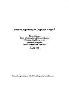
Spatial Correlation Degrades Performance

$ 91

Uncoded (i.i.d. fading) Uncoded (correlated fading) Uncoded SISO AWGN Rate−3/4 Turbo Coded (i.i.d. fading) Rate−3/4 Turbo Coded (correlated fading) Min. SNR for capacity = 48 bps/Hz (i.i.d. fading) Min. SNR for capacity = 48 bps/Hz (correlated fading)

0

10

−1

16x16 ILL−only STBC, 16−QAM Nt = Nr, LAS detection

−2

10

−3

10

−4

10

Min. SNR = 11.1 dB (i.i.d.) Min. SNR = 12.6 dB (correlated)

Bit Error Rate

10

Correlated MIMO channel parameters: fc = 5 GHz, R = 500 m, S = 30 dt = dr = 4 cm. Dr = Dt = 20 m. θt = θr = 90 deg.

−5

10

5

10

15

20 25 30 35 Average Received SNR (dB)

40

45

50

Figure5: Uncoded/coded BER performance of 1-LAS detector i) in i.i.d. fading, and ii) in correlated MIMO fading in [3] with fc

= 5 GHz, R = 500 m, S = 30,Dt = Dr = 20 m, θt = θr = 90◦ , and

dt = dr = 2λ/3 = 4 cm. 16 × 16 STBC, Nt = Nr = 16, 16-QAM, rate-3/4 turbo code, 48 bps/Hz.

&

Spatial correlation degrades performance.

%

'



Increasing # Receive Dimensions Helps!

$ 92

Nt = Nr = 12, uncoded Nt = 12, Nr = 18, uncoded Uncoded SISO AWGN Nt = Nr = 12, rate−3/4 turbo coded Nt = 12, Nr = 18, rate−3/4 turbo coded Min. SNR for Capacity = 36 bps/Hz (Nt = Nr = 12) Min. SNR for capacity = 36 bps/Hz (Nt = 12, Nr = 18)

0

10

−1

12x12 ILL−only STBC, 16−QAM Nt = 12, Nr = 12,18, 1−LAS detection

−2

−3

10

−4

10

Min. SNR = 12.6 dB (Nr = 12)

10

Min. SNR = 9.4 dB (Nr = 18)

Bit Error Rate

10

Correlated MIMO chl parameters: fc = 5 GHz, R = 500 m, S = 30 Nrdr = 72 cm, dt = dr D = D = 20 m r

t

θ = θ = 90 deg. t

r

−5

10

5

10

15

20 25 30 35 Average Received SNR (dB)

40

45

50

Figure 6: Effect of Nr > Nt in correlated MIMO fading in [3] keeping Nr dr constant and dt = dr .

Nr dr = 72 cm, fc = 5 GHz, R = 500 m, S = 30, Dt = Dr = 20 m, θt = θr = 90◦ , 12 × 12 ILL-only STBC,

&

Nt = 12, Nr = 12, 18, 16-QAM, rate-3/4 turbo code, 36 bps/Hz. Increasing # receive

dimensions alleviates the loss due to spatial correlation.

%

'



Channel Estimation in Large MIMO?

$ 93

• Training based channel estimation

– Send 1 Pilot matrix followed by Nd data STBC matrices

0110 11111 101000000 00000 11111 11111 00000 11111 00000 11111 0 1 1010 1000000 N 00000 11111 11111 10 101000000 1010 11100 000 11 00 00000 11111 N11 1 Pilot Matrix

Nd Data STBCs

Space

t

t

Nd Nt

Pilot Matrix

11111 00000 11111 00000 11111 00000 00000 11111 00000 11111 11111 00000 00000 0000 11111 1111 Data STBCs

time

1 Frame

∗ 1 frame length (in # of channel uses), T = (Nd + 1)Nt ∗ 1 pilot matrix length (in # of channel uses), τ = Nt

[coherence time]

– Obtain an MMSE estimate of the channel matrix during pilot phase – Use estimated channel matrix to detect data matrices using LAS detection – Iterate between detection and channel estimation &

%

'



MIMO Capacity with Estimated CSIR

$ 94

Hassibi-Hochwald (H-H) bound [F] on capacity with estimated CSIR: C

2

3 « H ˆ ˆ Hc Hc 5 + Nt (1 + γβd ) + γβp τ Nt σ 2ˆ γ 2 βd βp τ

T −τ 4 E logdet INt T

≥

„

Hc

70 60

Ergodic Capacity (bps/Hz)

16 x 16 MIMO System

Perfect CSIR 1P + 8D (H−H bound) 1P + 1D (H−H bound)

50 40 30 24 bps/Hz 21.3 bps/Hz 20

4.3 dB

0 −4

−2

0

2

7.7 dB

12 bps/Hz 10

4 6 8 Average SNR (dB)

10

12

14

16

Figure 7: H-H capacity bound for 1P+8D (T = 144, τ = 16, βp = βd = 1) and 1P+1D (T = 32, τ =

16, βp = βd = 1) training for a 16 × 16 MIMO channel.

———————————-

&

[F] B. Hassibi and B. M. Hochwald, How much training is needed in multiple-antenna wireless links?, IEEE Trans. on Information Theory, vol. 49, no. 4, pp. 951-963, April 2003.

%

'



How Much Training is Required?

$ 95

Figure 8: Capacity as a function of Nt with SNR = 18 dB and Nr = 12 [F]. For a given Nr , SNR (γ), and

&

coherence time (T ), there is an optimum Nt .

%

'



BER with Estimated Channel Matrix

$ 96

0

10

1P+1D;T=32; 12 bps/Hz 1P+8D;T=144; 21.3 bps/Hz 1P+24D;T=400; 23.1 bps/Hz 1P+48D;T=784; 23.5 bps/Hz Perfect CSIR; 24 bps/Hz

−1

Bit Error Rate

10

−2

10

16x16 ILL−only STBC Nt=Nr=16, 4−QAM Rate −3/4 turbo code 1−LAS detection Iterative Det/Est (4 iterns.)

−3

10

−4

10

−5

10

4

6

8

10

12

14

16

18

20

Average Received SNR (dB) Figure 9: Turbo coded BER performance of LAS detection and channel estimation as a function of co-

herence time,

T = 32, 144, 400, 784 (Nd = 1, 8, 24, 48), for a given Nt = Nr = 16. 16 × 16

ILL-only STBC, 4-QAM, rate-3/4 turbo code. Spectral efficiency and BER performance with estimated

&

CSIR approaches to those with perfect CSIR in slow fading (i.e., large T ).

%

'



On Optimum Nt for a given Nr and T

$ 97

0

10

Sys−I: Nt=Nr=16, 4−QAM, Rate−1/2 turbo, T=48 Sys−II: Nt=12,Nr=16, 4−QAM, Rate−3/4 turbo,T=48

−1

Bit Error Rate

10

Sys−I: 16x16 ILL−only STBC, 10.33 bps/Hz Sys−II: 12x12 ILL−only STBC, 13.5 bps/Hz Iterative Det/Est (4 iterns.)

−2

10

−3

10

−4

10

−5

10

5

6

7

8 9 10 11 12 Average Received SNR (dB)

13

14

15

Figure 10: Comparison between two 1P + Nd D training-based systems, one with a larger Nt than the other for a given Nr and T .

• System-II with Nt = 12 achieves a higher spectral efficiency 13.5 vs 10.33 bps/Hz at a lesser SNR 8.6 vs 8.9 dB than System-I with Nt = 16. &

%

'


On Optimum Nt for a given Nr and T Parameters

System-I

System-II

# Rx antennas, Nr

16

16

Coherence time, T

48

48

# Tx antennas, Nt

16

12

16 × 16

12 × 12

16

12

Training

1P+2D

1P+3D

βpopt

1.2426

1.4641

βdopt

0.8786

0.8453

Modulation

4-QAM

4-QAM

1/2

3/4

10.33 bps/Hz

13.5 bps/Hz

8.9 dB

8.6 dB

STBC from CDA Pilot duration, τ

Turbo code rate Spectral efficiency

&


SNR at 10−3 coded BER

$ 98

%

'



Maximum a posteriori (MAP) Detection

$ 99

• Consider square M -QAM

√ • Each entry of x belongs to a M -PAM constellation √ (q−1) (0) (1) • Let bi , bi , · · · , bi denote the q = log2 ( M ) constituent bits of xi

• xi can be written as xi =

q−1 X j=0

(j)

2j bi ,

i = 0, 1, · · · , 2dt − 1

• Let the bit vector b ∈ {±1}2qdt be written as iT h △ (q−1) (0) (q−1) (q−1) (0) (0) · · · b2dt −1 · · · b2dt −1 b = b0 · · · b0 b1 · · · b1 △

• Defining c = [20 21 · · · 2q−1 ], x can be written as

&

x = (I2dt ⊗ c)b

%

'



$ 100

MAP Detection • Rx signal model can be written as y =

H(I2dt ⊗ c) b + n | {z } △

= H′ ∈ R2dr dt ×2qdt

(j)

• MAP estimate of bi ,

i = 0, · · · , 2dt − 1,

bb(j) = i

arg max

a ∈ {±1}

p

j = 0, · · · , q − 1 is (j) bi

′

= a | y, H

• Complexity: Exponential in qdt &

%

'



$ 101

Probabilistic Data Association • Originally developed for target tracking • Used in digital communications as well • PDA – A reduced complexity alternative to a posteriori probability (APP) detector/decoder/equalizer – Has been applied in

∗ Multiuser detection in CDMA (Luo et al 2001, Huang and Zhang 2004, Tan and Rasmussen 2006)

∗ MIMO detection (Pham et al 2004, Latsoudas and Sidiropoulos 2005, Jia et al 2006)

∗ Turbo equalization (Yin et al 2004)

&

%

'



PDA Based Large-MIMO Detection

$ 102

• Iterative algorithm

– In each iteration, 2qnt statistic updates (one for each bit) are performed (j)

• Likelihood ratio of bit bi in an iteration is (j)

Λi

(j)

P y|bi

△

=

P |

= +1

(j) y|bi △

{z

= −1

(j)

= βi

• Received signal vector y can be written as y

=

(j) hqi+j bi

+

2n t −1 X l=0

|

△

ht : tth column of H

&

(j)

P bi

P } |

q−1 X

(j) bi △

(6)

+n

(7)

= +1

= −1 {z } (j)

= αi

(m)

hql+m bl

m=0

m6=q(i−l)+j

{z

}

e (interf erence+noise vector) =n

%

'



PDA Based Large-MIMO Detection △

△

(j)

$ 103

(j)

j− • Define pj+ p = +1) and = P (b i i = P (bi = −1) i (j)

e to be Gaussian • To compute βi , approximate the distribution of n

• Mean of y △

(j)

= E(y|bi = +1) = hqi+j + µj+ i

2n t −1 X l=0

△

(j)

q−1 X m=0

hql+m (2pm+ − 1) (8) l

m6=q(i−l)+j

j+ = −1) = µ = E(y|b µj− i − 2hqi+j i i

• Covariance of y Cji = σ 2 I2Nr p +

2n t −1 X l=0

&

q−1 X m=0

(9)

hql+m hTql+m 4pm+ (1 − pm+ ) (10) l l

m6=q(i−l)+j

%

'



PDA Based Large-MIMO Detection

$ 104

(j)

j • Using µj± i and Ci , P (y|bi = ±1) can be written as (j)

P (y|bi = ±1) =

j −1 T −(y−µj± (y−µj± i ) (Ci ) i )

e

1

(2π)nr p |Cji | 2

(11)

• Using (11), βij can be written as βij

j −1 j− T j −1 T −((y−µj+ (y−µj+ (y−µj− i ) (Ci ) i )−(y−µi ) (Ci ) i ))

= e (j)

(12)

(j)

(j)

• Compute Λi using αi and βi (j)

• Update the statistics of bi as

(j)

(j) P (bi

= +1|y) =

Λi 1+

(j) Λi

,

(j) P (bi

• This completes one iteration of the algorithm

&

= −1|y) =

1 1+

(j) Λi

(13)

%

'



$ 105

PDA Based Large-MIMO Detection (j)

(j)

• Updated values of P (bi = +1|y) and P (bi = −1|y) in (13) for all i, j are fed back as a priori probabilities to the next iteration

• Algorithm terminates after a certain number of iterations • At the end of the last iteration, (j) (j) b as +1 if Λ ≥ 1, and −1 otherwise – decide b i

i

• In coded systems (j)

– feed Λi ’s as soft inputs to the decoder

• Overall per-bit-complexity of the algorithm: O(n2t ) &

%

'



BER Performance of PDA

0

$ 106

0

10

10

Nt = Nr = 8 Nt = Nr = 16 Nt = Nr = 32 Nt = Nr = 64 Nt = Nr = 96 SISO AWGN

−1

10

LAS, 4x4 STBC PDA, 4x4 STBC Nt x Nt non−orthogonal ILL STBCs Nt = Nr, 4−QAM

−1

LAS, 8x8 STBC PDA, 8x8 STBC

10

LAS, 16x16 STBC PDA, 16x16 STBC SISO AWGN

−2

−2

−3

10

10 Bit Error Rate

Bit Error Rate

10

V−BLAST MIMO, Nt = Nr 4−QAM, m = 5

Performance improves with increasing Nt = Nr.

−4

10

0

BER improves with increasing Nt = Nr

10

−4

10

−5

10

Number of iterations m = 10 for PDA MMSE initial vector for LAS −3

−5

2

4

6

8

10


(a) V-BLAST, 4-QAM

12

14

16

10

0

2

4


12

14

16

(b) NO-STBC, 4-QAM

————————S. K. Mohammed, A. Chockalingam, B. S. Rajan, Low-complexity near-MAP decoding of large non-orthogonal STBCs using PDA, IEEE

&

ISIT’2009, Seoul, June 2009.

%

'



Algorithms for Inference

$ 107

• Graphical Models – graphs that indicate statistical dependence between random variables

• A set of algorithms that solve inference problems by passing messages on graphical models

– Belief Propagation

∗ Message passing algorithm initially formalized for Bayesian networks – Generalized Distributive Law (GDL)

∗ Solves the Marginalization of a Product Function (MPF) problem. Generalization of BP

– Sum Product (SP) algorithm

∗ Also solves the MPF problem on factor graphs. Another generalization of BP

&

%

'



$ 108

Graphical Models

• Three types of graphical models – Bayesian belief networks – Factor Graphs – Markov Random Fields

———— J. Pearl, Probabilistic Reasoning in Intelligent Systems: Networks of Plausible Inference, Morgan Kaufmann, San Mateo, California, 1988. B. J. Frey, Graphical Models for Machine Learning and Digital Communication, Cambridge: MIT Press, 1998.

&

%

'



$ 109

Factor Graphs • Bipartite graph – Variable nodes and function nodes. Undirected edges allowed between variable and function nodes only

• Explicitly portray factorization of a global function into local functions

• If f (x) is a global function that factorizes into NF local functions as f (x) ∝

NF Y

fj (xj )

j=1

• Variable nodes represent the variables in x. Function nodes represent local functions fj (xj ) &

%

'



BP on Factor Graphs

$ 110

• BP: A special case of sum-product (SP) algorithm [G]. Global function is the joint probability distribution

• Message from variable node x to function node f mx→f (x) =

Y

mh→x (x)

h∈N (x)\{f }

• Message from function node f to variable node x mf →x (x) =

X h

f (xf )

x\{x}

• Belief at variable node x is bx→f (x) =

Y

my→f (y)

y∈N (f )\{x}

Y

i

mh→x (x)

h∈N (x)

————[G] F. R. Kschischang, B. J. Frey, H. A. Loeliger, Factor graphs and the sum-product algorithm, IEEE Trans. on Information Theory, vol. 47, no. 2,

&

February 2001.

%

'



$ 111

Loopy Belief Propagation • BP is proven to work in cycle-free graphs – gives exact marginals

• BP is often successful in loopy graphs also – e.g., Turbo decoding

• BP message passing, when applied in loopy graphs, is called loopy BP – gives only ‘estimates’ of marginals – works well in several applications

&

%

'



Large-MIMO Detection using BP on FGs

$ 112

• Each entry of the vector y is treated as a function node (observation node) • Each symbol, xi ∈ {±1}, is treated as a variable node • A key ingredient: Gaussian approximation of interference (GAI) interf erence

yi

= hik xk +

z

Nt X

}|

hij xj + ni ,

j=1,j6=k

|

is modeled as CN (µzik , σz2ik ) with µzik =

Nt X

{

△

{z

= zik

(14)

}

hij E(xj ),

(15)

|hij |2 Var(xj ) + σ 2 ,

(16)

j=1,j6=k

σz2ik =

Nt X

j=1,j6=k

where hij is the (i, j)th element in H &

%

'



Large-MIMO Detection Using BP on FGs

$ 113

• With xi ’s ∈ {±1}, the log-likelihood ratio (LLR) of xk at observation node i, denoted by Λki , is Λki

4 p(yi |H, xk = 1) = 2 ℜ (h∗ik (yi − µzik )) = log p(yi |H, xk = −1) σzik

(17)

• LLR values computed at observation nodes are passed to variable nodes • Using these LLRs, variable nodes compute the probabilities PNr k Λ exp ( △ l) l=1,l6 = i k+ pi = pi (xk = +1|y) = PNr 1 + exp( l=1,l6=i Λkl )

(18)

and pass them back to the observation nodes

• This message passing is carried out for a certain number of iterations

• At the end, xk is detected as &

x bk = sgn

Nr X i=1

Λki

(19)

%

'



$ 114

Message Passing on FGs with GAI

x1

p1+ i

Λ1i = f ({pj+ i }, j 6= 1)

x1

y1

Λk1

Eqn. (17),(15),(16)

p2+ i x2

pni t +

yi

k pk+ 1 = g({Λl }, l 6= 1)

y1

Eqn. (18)

Λ2i x2

Λk2 y2

Λni t

xnt

xnt

Λknr

xk

pk+ 2 y2

pk+ nr

y nr

y nr

Figure 11: Message passing between variable nodes and observation nodes

• Per-symbol complexity: O(Nt )

&

%

'


Performance of BP on FGs with GAI

0

10

Nt = Nt; 4−QAM # BP iterations = 20 Message damping factor = 0.4

BER improves with increasing Nt

−1

−1

−2

10

8x8 VBLAST −3

10

16x16 VBLAST 24x24 VBLAST

−4

10

Nt=Nr; 4−QAM; STBCs from CDA # BP iterations = 20 Message damping factor = 0.4

10

Bit Error Rate

10

Bit Error Rate

$ 115

0

10

−2

10

−3

10

4x4 STBC 8x8 STBC

32x32 VBLAST −4

10

64x64 VBLAST

16x16 STBC SISO AWGN

SISO AWGN −5

10


0

−5

2

4

6

8

Average received SNR (dB) (a) V-BLAST

10

12

10

0

2

4

6

8

10

12


(b) NO-STBC

• BP with GAI achieves near-optimal performance for increasing # dimensions ————

[H] P. Som, T. Datta, A. Chockalingam, B. S. Rajan, Improved large-MIMO detection using damped belief propagation, IEEE ITW’2010, Cairo,

&

January 2009.

%

'



Markov Random Fields

$ 116

• MRFs are undirected graphs

– Vertices are random variables. Edges represent conditional dependence

• Statistical dependencies among the variables are such that any variable is independent of all other variables, given its neighbors

• Variables are constrained by compatibility functions or clique potentials • Clique: A fully connected sub-graph

– A clique is maximal if it is not a strict subset of another clique

• Let Nc be the # maximal cliques, and xj be the variables in maximal clique j • Let ψj (xj ) be the compatibility function of clique j

• Then the joint distribution of the variables is given by

&

Nc 1 Y ψj (xj ) , p (x) = Z j=1

Z : Partition Function

%

'



MRFs

$ 117

• Consider r.v.s x1 , . . . , x5 such that p (x1 , x2 , x3 , x4 , x5 )

= p (x1 ) p (x2 |x1 ) p (x3 |x1 , x2 )

p (x4 |x1 , x2 , x3 ) p (x5 |x3 , x4 )

• The MRF for x1 , . . . , x5 is x1

x3

x5

x2

x4

• Maximal cliques {x1 , x2 , x3 , x4 } and {x3 , x4 , x5 } • Joint probability distribution is

&

p (x) =

1 ψ1 (x1 , x2 , x3 , x4 ) ψ2 (x3 , x4 , x5 ) . Z

%

'



Pairwise MRFs

• Pairwise MRF

x1

– All cliques in the MRF are of size 2

x2 y1

– Clique potentials are all functions of two variables

y2

y4

• xi ’s: hidden variables. yi ’s: observed variables

x7

p (x, y)

∝

i,j

y6

y5 x9

y8

y9

Joint compatibility function φi (xi , yi )

• Joint probability distribution takes the form [I] Y

y3 x6

x8

y7

• Compatibility function ψi,j (xi , xj ).

x3

x5

x4

$ 118

ψi,j (xi , xj )

Y

φi (xi , yi )

i

————[I] J. S. Yedidia, W. T. Freeman, Y. Weiss, Understanding belief propagation and its generalizations, MERL Tech. Rep. TR-2001-22, January

& 2002.

%

'



$ 119

BP on MRFs • Consider observed variables yi ’s as fixed. Write joint compatibility function φi (xi , yi ) as φi (xi ) • Joint distribution is:

p (x)

∝

Y

ψi,j (xi , xj )

i,j

Y i

• Message from node i to node j is [I] mi,j (xj ) =

X

φi (xi )

φi (xi ) ψi,j (xi , xj )

xi

Y

mk,i (xi )

k∈N (i)\j

• Final belief at node i about xi is computed as bi (xi )

&

∝ φi (xi )

Y

mj,i (xi )

j∈N (i)

%

'



MRF of a MIMO System

• MRF of V-BLAST MIMO system: fully connected graph

$ 120

x1

x8

x2

• MRF for 8 × 8 V- BLAST MIMO: x7

x3

x4

x6

x5

• MRF of MIMO system has pairwise interactions with edge and self potentials [H] ψi,j (xi , xj ) = exp −xi ℜ{Rij }xj φi (xi ) = exp xi ℜ{zi } + ln p(xi )

where Rij is the i, j th element of the matrix R element of the vector z &

△ 1 H H y. 2 σ

=

△ 1 = σ2 HH H,

(20) (21)

and zi is the ith

%

'



Message Passing in MIMO MRF

$ 121

• bi (xi ): belief at node i,

xi ∈ {±1} – proportional to how likely xi was transmitted

• mj,i (xi ): message from node j to node i – proportional to how likely xj thinks xi was transmitted • Belief at node i is

bi (xi )

• Messages are defined as mj,i (xi ) ∝

X xj

∝ φi (xi )

Y

mj,i (xi )

(22)

j∈N (i)

φj (xj ) ψj,i (xj , xi )

Y

mk,j (xj )

(23)

k∈N (j)\i

• Eqn. (23) actually constitutes an iteration. terminate after a finite # iterations. • Final belief is a soft-output

– in uncoded systems, detect x bi ’s from beliefs – in coded systems, can feed beliefs directly to the decoder &

%

'


Damped Belief Propagation

• Message Damping

(t) m e i,j (xj )

∝

X

φi (xi ) ψi,j (xi , xj )

xi

(t−1)

(t)

where αm

(t−1)

mk,i

(xi ) ,

(t)

(xj ) + (1 − αm ) m e i,j (xj ),

∈ [0, 1) is the message damping factor

• Belief Damping

(t)

bi

&

Y

$ 122

k∈N (i)\j

mi,j (xj ) = αm mi,j

where αb


(t) e bi (xi )

∝ φi (xi ) (t−1)

(xi ) = αb bi

Y

(t)

mj,i (xi ),

j∈N (i)

(t) (xi ) + (1 − αb ) e bi (xi ),

∈ [0, 1) is the belief damping factor

%

'



Performance of Damped BP in Large-MIMO Detection −1

$ 123

0

10

10

Nr=Nt=16 Nr=Nt=24 SISO AWGN

Nt=Nr=4 Nt=Nr=8 Nt=Nr=16 Nt=Nr=24 Nt=Nr=32 SISO AWGN

V−BLAST, BPSK, message damped BP Message damping factor αm = 0.2 # BP iterations = 5

−1

10

−2

Bit Error Rate

Bit Error Rate

10

V−BLAST, BPSK Average received SNR = 8 dB Message damped BP # BP iterations = 5

−3

10

−2

10

−3

BER improves with increasing Nt=Nr

10

−4

10

−4

10

0

−5

0.1

0.2

0.3

0.4

0.5

0.6

0.7

0.8

0.9

1

10

0

Message Damping Factor (α m)

(c) Performance as a function of damping factor

1

2

3

4

5

6

7

8

9

10


(d) Performance as a function of SNR

• Damping significantly improves performance • Per-symbol complexity: O(Nt Nr ) ————

January 2010. &

P. Som, T. Datta, A. Chockalingam, B. S. Rajan, Improved large-MIMO detection using damped belief propagation, IEEE ITW’2010, Cairo,

%

'



$ 124

Markov Chain Monte Carlo (MCMC) Methods • In MCMC methods, statistical inferences are developed by simulating the underlying processes through Markov chains

• By doing so, it becomes possible to reduce exponential detection complexity to linear/polynomial complexities.

• MCMC techniques have been reported in the context of CDMA and MIMO detection

———— R. Chen, J. S. Liu, and X. Wang, Convergence analyses and comparisons of Markov chain Monte Carlo algorithms in digital communications, IEEE Trans. on Signal Processing, vol. 50, no. 2, pp. 255-270, Feb 2002. B. Farhang-Boroujeny, H. Zhu, and Z. Shi, Markov chain Monte Carlo algorithms for CDMA and MIMO communication systems, IEEE Trans. on Signal Processing, vol. 54, no. 5, pp. 1896-1909, May 2006. H. Zhu, B. Farhang-Boroujeny, and R. R. Chen, On performance of sphere decoding and Markov chain Monte Carlo methods, IEEE Signal Processing Letters, vol. 12, no, 10, pp. 669-672, Oct 2005.

&

%

'



MCMC Method

$ 125

• Sampling from complicated distributions is often difficult • In MCMC, sampling from a complicated n-dimensional distribution, say p(x), is done by

– defining a Markov chain over the state space of x, and – sampling over the transition probability distributions of the Markov chain

• The transition probability distributions of the Markov chain should have the following properties:

– Drawing samples should be easy – Markov chain must be irreducible – Steady state distribution of the Markov chain should be the target distribution, i.e., p(x)

&

%

'



$ 126

Gibbs Sampling • Widely used sampling method • Applicable when the conditional distribution of each variable is known, and is easy to sample from

– Conditional distributions, often being Gaussian (or other common distributions), are far easier to simulate

• Samples in a Gibbs sequence, after burn-in period, converge to a stationary distribution that is independent of starting values

• This stationary distribution is the target distribution we are trying to simulate &

%

'



$ 127

MCMC Based MIMO Detection • Joint probability distribution of interest in MIMO detection is given by −ky − Hxk2 p(x|y, H) = p(x1 , · · · , xnt |y, H) ∝ exp 2σ 2

(24)

• MIMO detection problem can be solved using MCMC simulations – can use Gibbs sampling, since the sampling distribution in this problem is well known (Gaussian)

• Polynomial complexity in nt &

%

'



Detection Using Gibbs Sampling

$ 128

• Initialize an initial bit vector x(t=0) • In each iteration of the algorithm (t = 1, 2, 3, · · · ), obtain an updated vector by sampling from conditional distributions as follows: (t+1)

x1

(t+1)

x2

(t+1)

x3

(t)

(t)

(t+1)

, x3 , · · · , x(t) nt ),

∼ p(x1 |x2 , x3 , · · · , x(t) nt ),

∼ p(x2 |x1

(t+1)

∼ p(x3 |x1

(t)

(t+1)

, x2

.. .

(t+1)

x(t+1) ∼ p(xnt |x1 nt

(t+1)

, x2

(t)

, x4 , · · · , x(t) nt ), (t+1)

, · · · , xnt −1 ).

(25)

• Repeat the iterations N times • Detected vector in a given iteration

– choose that vector which has least ML cost in all iterations up to that iteration &

%

'



BER Performance of Conventional MCMC

$ 129

0

10

16X16 V−BLAST MIMO, 4−QAM

−1

Bit Error Rate

10

−2

10

Conventional MCMC Sphere Decoder

−3

10

−4

10

0

2

4

6

8

10

12


• Problem in conventional MCMC based detection – Stalling problem at high SNRs

∗ at high SNRs, the Markov chain associated with conventional MCMC ∗ &∗

becomes nearly reducible Transition probabilities from some states to other states become very low Hence, BER performance degrades at high SNRs

%

'



$ 130

MCMC Algorithm in [J] • The MCMC algorithm in [J] used the joint distribution as ky − Hxk2 , p(x1 , · · · , xnt |y, H) ∝ exp − 2α2 σ 2 where α is a temperature parameter

(26)

• Uses fixed value of α in all the iterations • Performance is highly dependent on the temperature value α • Optimum value of α varies with SNR and nt , making the algorithm less attractive ———— [J] M. Hansen, B. Hassibi, A. G. Dimakis, W. Xu, Near-optimal detection in MIMO systems using Gibbs sampling, IEEE ICC2009, Honolulu, December 2009.

&

%

'



Performance of MCMC Algorithm in [J]

$ 131

0

10

16X16 V−BLAST MIMO, 4QAM

−1

Bit Error Rate

10

−2

10

α=1.5 α=2 α=3 Sphere Decoder

−3

10

−4

10

0

2

4

6

8

10

12


• Performance is highly dependent on the value of α • Optimum value of α varies with SNR and nt • Stalling problem persists

&

%

'



A Randomized MCMC Algorithm

$ 132

• Observation – ML cost of the updated vectors obtained through conventional Gibbs sampling gets stagnant for many iterations – Implies that the solution vector is not updating itself with the iterations

• Idea – Try randomization of the update rule in the sampling – Do not to use conventional Gibbs sampling always, but, in addition, probabilistically use a randomized sampling as well

• Motivation – To avoid stagnancy of the ML cost, thereby allowing the solution vector to update itself with iterations

&

%

'



A Randomized MCMC Algorithm

$ 133

• Conventional Gibb’s sampling –

(t)

xi ’s are updated as per (25) with probability 1

• Randomized MCMC (R-MCMC) [K] (t)

– Update xi ’s as per (25) with probability (1 − qi ) and use a different update rule with probability qi = n1 t – Different update rule is as follows: ∗ Generate |A| probability values from uniform distribution as (t)

p(xi = j) ∼ U [0, 1], ∀j ∈ A such that

|A| X

(t)

p(xi = j) = 1

j=1

(t)

∗ sample xi from this generated pmf • This simple randomization approach significantly alleviates stalling problem ————

&

[K] Ashok Kumar, Suresh Chandrasekaran, A. Chockalingam, B. S. Rajan, Near-optimal large-MIMO detection using randomized MCMC and randomized search algorithms, IEEE ICC2011, Kyoto, June 2011.

%

'



Performance of R-MCMC Algorithm

$ 134

• 16 × 16 MIMO, 4-QAM 0

10

16x16 V−BLAST MIMO, 4−QAM

−1

Bit Error Rate

10

−2

10

MCMC in [J], α=1 MCMC in [J], α=1.5 MCMC in [J], α=2 MCMC in [J], α=3 Proposed R−MCMC Sphere Decoder

−3

10

−4

10

0

2

4

6

8

10

12


• R-MCMC significantly alleviates stalling problem • R-MCMC achieves almost sphere decoding performance

&

%

'



Performance/Complexity of R-MCMC Algorithm O(n2t ) per-symbol complexity

BER improves with increasing nt 0

19

V−BLAST MIMO, 4−QAM −1

−2

10

8x8

−3

10

8x8, Sphere Decoder 8x8, Proposed R−MCMC 16x16, Sphere Decoder 16x16,Proposed R−MCMC 32x32,Proposed R−MCMC 64x64,Proposed R−MCMC Unfaded SISO AWGN

−4

10

16x16

−5

0

2

4

6

V−BLAST MIMO, 4−QAM, BER=0.01 18 17 16 15 14 Proposed R−MCMC 2 O(nt )

13

2

Bit Error Rate

10

log (Average No of real Operations)

10

10

$ 135

8


(e) BER Performance

10

12

O(nt)

12 11 8

16

32

64

Nt

(f) Complexity

• R-MCMC achieves near-ML performance with O(n2t ) per-symbol complexity

&

%

'



Large-MIMO Applications/Standardization

$ 136

• Potential Applications

– Fixed Wireless HDTV/3DTV distribution – High-speed back haul connectivity between BSs/BSCs – High-rate links between wireless mesh network nodes

• Large-MIMO in Wireless Standards?

– Multi-Gigabit Wireless LAN/PAN (IEEE 802.11ac, 5GHz / 802.11ad, 60 GHz)

∗ 802.11ac (WiFi-Advanced) considers 8 × 4, 16 × 2 MU-MIMO, 8 × 8 MIMO ∗ Can consider adopting more number of antennas – LTE-Advanced

∗ LTE-A has adopted 8 × 8 MIMO. ∗ Can consider adopting more number of antennas (e.g., 12 × 12, 16 × 16)

&

%

'



Concluding Remarks

$ 137

• Gigabit wireless networking is fast becoming a reality • Large-MIMO: A key enabler of multi-gigabit wireless • Gigabit wireless research directions – PHY layer

∗ Large-MIMO techniques · signal detection, channel estimation, compact antenna design – Higher layers

∗ high throughput MAC protocols for gigabit wireless ∗ Applications in gigabit networks

&

%

'



Concluding Remarks

$ 138

• Low-complexity large-dimension wireless communications – nascent – promising

• ‘Large-dimension behavior’ of algorithms – can be exploited well in wireless communications

• Potential benefits – increased spectral efficiency – increased diversity orders – and more..

&

%

'



$ 139

Thank You

&

%

Low-Complexity Algorithms for Large-MIMO ... - Semantic Scholar

Low-Complexity Algorithms for Large-MIMO ... - Semantic Scholar

Suggest Documents

Genetic Algorithms - Semantic Scholar

Cultural Algorithms - Semantic Scholar

Memetic Algorithms - Semantic Scholar

algorithms - Semantic Scholar

Evolutionary Algorithms - Semantic Scholar

Semantic Matchmaking Algorithms - Semantic Scholar

Semantic Matchmaking Algorithms - Semantic Scholar

Hierarchical Clustering Algorithms for Document ... - Semantic Scholar

Asymptotically Faster Algorithms for the ... - Semantic Scholar

Iterative Algorithms for Graphical Models - Semantic Scholar

Algorithms for duplicate documents - Semantic Scholar

Online Competitive Algorithms for Maximizing ... - Semantic Scholar

Consistency Check Algorithms For MulTI ... - Semantic Scholar

Hierarchical Temporal Memory Algorithms for ... - Semantic Scholar

Genetic algorithms for designing multihop ... - Semantic Scholar

Sequential Importance Sampling Algorithms for ... - Semantic Scholar

Transfer Learning Algorithms for Image ... - Semantic Scholar

Enumeration Algorithms for Maximal Perfect ... - Semantic Scholar

Algorithms for Arithmetic Circuits - Semantic Scholar

EFFICIENT ALGORITHMS FOR INFERENCES ON ... - Semantic Scholar

Semidefinite Programming Algorithms for Sensor ... - Semantic Scholar

Conjugate Gradient Algorithms for Minor ... - Semantic Scholar

Comparison of different algorithms for ... - Semantic Scholar

OptimizationâBased Decoding Algorithms for ... - Semantic Scholar

Low-Complexity Algorithms for Large-MIMO ... - Semantic Scholar