Semidefinite Programming Algorithms for Sensor Network Localization using. Angle of Arrival Information. Pratik Biswas, Hamid Aghajan, Yinyu Ye. Wireless ...
Semidefinite Programming Algorithms for Sensor Network Localization using Angle of Arrival Information Pratik Biswas, Hamid Aghajan, Yinyu Ye Wireless Sensor Networks Laboratory, Dept. of Electrical Engineering, Stanford University Room 318 , 161 Packard Building, 350 Serra Mall, Stanford, CA-94305 pbiswas,haghajan,yyye @stanford.edu Abstract The problem of position estimation in sensor networks using a combination of distance and angle information as well as pure angle information is discussed. For this purpose, a semidefinite programming relaxation based method that has been demonstrated on pure distance information is extended to solve the problem. Practical considerations such as the effect of noise and computational effort are also addressed. In particular, a random constraint selection method to minimize the number of constraints in the problem formulation is described. The performance evaluation of the technique with regard to estimation accuracy and computation time is also presented by the means of extensive simulations.
1. Introduction Localization or position estimation in sensor networks has a wide variety of applications including target tracking, routing, asset location etc. In general, the information collected by a sensor node is more meaningful if we are also aware of its position The localization problem usually involves estimating positions of the nodes in a sensor network based on a mixture of mutual distance, angle or proximity constraints. Existing methods exploit a variety of techniques including iterative triangulation multidimensional scaling and convex programming. In particular, the use of Semidefinite Programming relaxations has been demonstrated for the localization problem in [2]. The technique lends a nice interpretation to the localization problem under the general framework of Euclidean distance geometry. The technique is especially appealing in the scenario where we wish to exploit the collaborative nature of sensor networks in order to use the mutual information between the sensor nodes. While this does not allow the technique to be purely distributed (where each sensor node can infer its position on its own), it takes advantage of the collective information shared between a network of nodes, thus leading to more precise position determination. While the application of SDP relaxations to pure distance information has been discussed in previous work, a framework does not exist where we can use this technique for angle information. Solving this problem is particularly useful in a scenario where we use sensors that are also able to detect mutual angles, like in image sensor nodes. This paper takes a step in this direction by extending the SDP model to solve the localization problem using angle information in combination with distance information, or independently. The performance of this tech-
nique with respect to different factors is also evaluated.
2. Background The use of angle information for sensor network localization has been investigated by Niculescu and Nath [6]. It is assumed that the network has a few landmark or anchor points whose positions are already known. The algorithm uses information between the anchors and unknown points to set up triangulation equations in order to determine positions of unknown points. The calculated positions are then forwarded to other unknown points and used in further triangulation. It is often useful to consider methods that exploit the collective information between the nodes in a centralized fashion. A technique using linear bounding hyperplane based constraints is described in Doherty et al [4]. However, the constraints may be too loose to provide a meaningful solution. Our method also attempts to solve the position estimation problem in one step by solving the problem using global information. This avoids the issue of forwarding and also error propagation as in [6]. Furthermore, by using global information, it is hoped that solutions are more accurate. Our method can provide an alternative to [4] with tighter constraints. The quadratic programming formulation of the distance geometry problem with distance information will serve as a good starting point to the discussion. Suppose that we have m known points ak ∈ R 2 , k = 1, ..., m, and n unknown points x j ∈ R 2 , j = 1, ..., n. Let Na be the set of k, j and Nu be the set of i, j indices for which the Euclidean distance measures dk j corresponding to the distance between the points ak and x j , or di j corresponding to the distance between the points xi and x j are known. The distance measures may be corrupted with noise. Then, the quadratic model problem can be defined by ∑i, j |αi j | + ∑k, j |αk j |
min s.t.
kxi − x j kak − x j
k2
k2
= (di j
)2 + α
i j , ∀i, j ∈ Nu , 2 = (dk j ) + αk j , ∀k, j ∈ Na ,
(1) (2) (3)
Other sophisticated models that handle noisy distance information more effectively by minimizing other objectives can also be developed. Let X = [x1 x2 ... xn ] be the 2 × n matrix that needs to be determined. Then kxi − x j k2 = eTij X T Xei j kak − x j k2 = (ak ; e j )T [I X]T [I X](ak ; e j ), where ei j is the vector with 1 at the ith position, −1 at the jth position and zero everywhere else; and e j is the vector of all zero except −1 at the jth position. We can obtain a formulation
of the problem in the matrix form. Unfortunately this problem is not convex. Previous approaches have completely ignored the nonconvex constraints [4]. The approach described in [2] retains them but relaxes the entire problem into a standard SDP problem. Let Y = X T X. We relax this constraint to Y º X T X. Basically, this technique is a rank constraint relaxation that is also a key idea in solving other NP hard quadratic programs using SDP. This as a matrix linear inequality [3] µ can be formulated ¶ I X Z= º 0 So the problem reduces to a set of linXT Y ear constraints and a linear matrix inequality and can therefore be solved as an SDP. The SDP formulation is min
∑i, j |αi j | + ∑k, j |αk j |
(4)
s.t.
(1; 0; 0)T Z(1; 0; 0) = 1
(5)
(0; 1; 0)T Z(0; 1; 0) = 1
(6)
(1; 1; 0)T Z(1; 1; 0) = 2
(7)
(0; ei j
)T Z(0; e
2 i j ) = (di j ) + αi j , ∀i, j ∈ Nu ,
B N
C
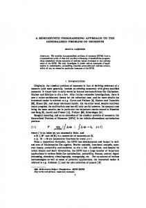
Figure 1. Sensor, Axis orientation and field of view
seen from sensor j can be expressed as (x j − xi )T (x j − xl ) = cos θi jl , or d ji d jl kxl − xi k2 = d 2ji + d 2jl − 2d ji d jl · cos θi jl
(8)
(ak ; e j )T Z(ak ; e j ) = (dk j )2 + αk j , ∀k, j, ∈ Na
(9)
Z º 0.
(10)
Axis orientation
A
(11)
where θi jl is the angle between sensor i and sensor l as seen from sensor j, d ji is the distance between sensor j and sensor i and d jl is the distance between sensor j and sensor l. A similar equation can also be derived when an anchor ak is involved. Now by applying the SDP relaxation described before in Section 2 to convert the equations of type into linear equations and adding a linear matrix inequality, the problem consisting of the quadratic constraints of the type described above can be reduced once again to an SDP form.
A detailed analysis of this approach and experimental results are presented in [2].
3. Integrating Angle Information The scenario for which we will describe our algorithm is very similar to that described in [6]. Consider n unknown points x j ∈ R 2 , j = 1, ..., n. All angle measurements are made at each sensor relative to its own axis. The orientation θi of the axis with respect to a global coordinate system after a random deployment of the network is not known. There are also a set of m anchor nodes ak ∈ R 2 , k = 1, ..., m, that is, nodes whose positions are known a priori. Every sensor can detect neighboring sensors which are within its field of view and a specified communication range of it. The field of view is limited by the maximum angle (on either side of the axis) that the sensor can detect with respect to its own axis. Depending on the type of sensing technology used, these parameters can be accordingly set.Since every measurement is with respect to the axis of a sensor node at every unknown sensor, we also have angle measurements corresponding to the angle between 2 other sensors (either anchors or unknown) as seen from the sensor if the 2 sensors are within communication distance range of it and within its field of view. For a set of three points like in (Figure 1), we have the angle φi jk between xi and xk as seen from x j . The objective now is to find the positions of the unknown nodes. From the position information, we can also derive the orientation information.
3.2. Pure Angle Information Next we will consider the localization problem for pure angle information. The problem can be formulated in a variety of ways depending upon how we choose to exploit the angle constraints in our equations. The idea is to maintain the Euclidean distance geometry ’flavor’ in our approach where the quadratic term in the formulation is simply relaxed into an SDP. With this aim in mind, the following solution is presented. The same situation (with regard to angle measurements) as considered in the case of combined distance and angle information will be used here as well. The only difference is that absolutely no distance information between sensors is available. Consider 3 points xi , x j and xk that are not located on the same
B
C
r
O
3.1. Distance and Angle Information The first case we will consider is when we have both angle and distance information. We define a set Nb corresponding to triplets of points. For a set of three points in Nb , we have the angle θk ji between ak and xi as seen from x j as well as the distance d jk and d ji ; or the angle θi jl between xi and xl as seen from x j as well as the distance d ji and d jl . The angle information between unknown sensors i and l as
A
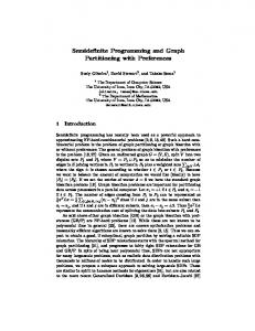
Figure 2. 3 points, the circumscribed circle and related angles, hAOBi = 2hACBi
2
line. One basic property concerning circles is that the angle sub-
tended by 2 of these points , say xi and xk at the center of the circle that circumscribes the 3 points is twice the angle subtended by the 2 points at the third point x j (Figure 2) . Let the radius of the circumscribing circle be ri jk , which is also unknown. Then by a simple application of the cosine law (similar to the one described in the previous section) on the triangle with the points xi , xk and the center of the circle. kxi − xk k2 = ri2jk + ri2jk − 2ri jk ri jk cos 2φi jk Therefore kxi − xk k2 = 2ri2jk (1 − cos 2φi jk )
being computationally tractable is a further research topic. The SDP solution can also serve as a good starting point for local refinement through a local optimization method. This idea has been explored for distance based information in [5]. Extending gradient based refinement ideas for angle information is being pursued. Because we consider triplets of points, the number of angle constraints of type in Equations (3.1) and (12) increase very substantially (O(n3 )) as the network size(n) and radio range(R) increases. It is very inefficient to include all the angle constraints if only a few of them can be used to obtain the solution. The problem becomes too strictly overdetermined when in fact most of the constraints are redundant and the problem can be solved using only a subset of the constraints. For example, even for a network size of 40, the number of constraints for a radio range of 0.3 and omnidirectional angle measurements is about 1100. Clearly, the problem starts becoming intractable for even such small cases. Therefore, we propose an intelligent constraint generation methodology that can help in keeping the number of constraints selected small enough such that the problem is tractable. In selecting the constraints, we try ensure that the constraints selected are well distributed in terms of the points that they correspond to, that is, there are not too many or too few constraints arising from angle relations for a single point in the network . This can be done by limiting the number of constraints that arise from angle relations for a particular point below a particular threshold. Furthermore, the constraints are between pairs of points. So the constraint selection should not concentrate only on angle constraints corresponding to a particular pair of points as seen from other points. While this can be done by keeping a counter of the number of constraints on every possible pair, clearly this strategy adds a lot of overhead to the actual processing. In order to minimize the cost of the constraint selection, we use a randomized constraint selection technique where a constraint is added to the problem with a certain probability. This probability can be made to depend upon number of desired constraints as a fraction of the total number of possible constraints. The randomized selection ensures that the constraints take into account the global information of the network as opposed to smaller local clusters of points. While the above mentioned methods work well for networks of up to 70-80 points, severe scalability issues will arise for very large networks of say, thousands of points. We are in the process of developing a distributed method for angle information. Such an algorithm will be similar in spirit to that described in [1] for pure distance information. The entire network will be divided into clusters using anchor information and the smaller SDPs solved for each cluster. The cluster idea still takes advantage of the collective information between a set of nodes which are within a cluster. For points in clusters that are well separated from each other, there is little or no mutual information to begin with. So the problem can be solved in a parallel and ’decoupled’ fashion in each of the separate clusters. The computations can be made iterative such that points that were well estimated can be used in subsequent iterations to provide estimates for points that were poorly estimated in previous iterations. Information about points that are on the boundary of 2 clusters can even be exchanged between clusters in order to assist in localizing other points within them. In the case of noisy angle information, the placement of anchors assumes a critical role for both approaches. If the anchors are placed in the interior of the network, the estimations
(12)
We can create a similar set of equations in the unknowns xi , x j , xk and ri2jk using the angles between all such sets of points. These sets of equations can be generated for all sets of points that have mutual angle information with each other. For each set of 3 points, a new unknown ri2jk is introduced. It can be observed that once again the constraints are quadratic in the matrix X = [x1 x2 . . . xn ]. By applying the SDP relaxation , that is, using the substitution Y = X T X and relaxing this constraint to Y º X T X, the problem is reduced once again to an SDP with one matrix linear inequality and some linear constraints, with the unknowns Y, X, ri2jk . Furthermore, we can also include the linear constraints introduced by angle measurements at the anchors as described in equation (??). It is pertinent to ask if the introduction of new unknowns ri2jk will cause the problem to be underdetermined. The matrix Y has n(n + 1)/2 unknowns and X has 2n unknowns. Suppose the number of triplets that have mutual angle information amongst each other is k. The angle measurements considered are exact, that is, they do not have any error. Then k more unknowns corresponding to the radii of the circumscribing circles are introduced. At the same time, we have constraints for each circle, so a total of 3k constraints exist. Hence as long as 3k > k + n(n + 1)/2 + 2n, the set of equations will have a unique feasible solution. The matrix X ∗ = [xˆ1 xˆ2 . . . xˆn ] and Y ∗ = (X ∗ )T X ∗ where xˆi is the true position of the sensor i, will be the solution satisfying these equations. Therefore if k is large enough, the unique solution ¡¢ will exist. The maximum possible value of k is in fact n3 . If however, the connectivity is high, then the size of the triplet set k is also large enough for the set of equations to have a unique solution.
4. Practical Considerations In realistic scenarios, the angle information is not entirely accurate. So softer SDP models that minimize the errors in the constraints can be developed based on constraints discussed in the previous section by introducing slack variables. Note that our formulation allows flexibility in choosing any combination of exact or inexact distance and angle constraints depending on the information provided. For example, for a constraint of the type in Equation (12) kxi − xk k2 = 2ri2jk (1 − cos 2φi jk ) With noisy angle information, it can be modified to kxi − xk k2 = 2ri2jk (1 − cos 2φi jk ) + αi jk . where αi jk is the error in the equation. We can now choose to minimize an objective function corresponding to the resulting SDP, the absolute sum of these errors. We can also choose alternative objective functions, such as sum of error squares, that penalize the errors in the equations differently. The choice a suitable objective function to minimize that gives the best performance for a particular noise model while
3
4 anchors, Pure angle
for points outside the convex hull of the anchor points also tend to be towards the interior of the network and are therefore quite erroneous. This problem does not present itself when the anchors are placed on the perimeter of the network. Therefore for our simulations, we place four anchors each on the corners of a square network. The estimation error is reduced significantly by doing this. We argue that this assumption that anchors are placed on the perimeter of the network is reasonable in a range of position estimation scenarios since during deployment of a network, we should be aware of the overall area in which it it to be deployed. The placement of powerful anchor nodes on the perimeter of this area is a feasible assumption. Other anchors may be deployed randomly in the interior like the rest of the nodes. The reason for this behavior is not entirely clear and more research is required to rigorously establish it. This analysis will also help in developing formulations that are less sensitive to error placement and to also devise efficient anchor placement strategies.
4 anchors, Distance and Angle 25
45 40
20
30 25 20
R=0.3 R=0.4 R=0.5 R=0.6 R=0.7
Error (%R)
Error (%R)
35 15
R=0.3 R=0.4 R=0.5 R=0.6 R=0.7
10
15 10
5
5 0.05
0.1
0.15 nf
0.2
0 0.05
0.25
0.1
0.15 nf
0.2
0.25
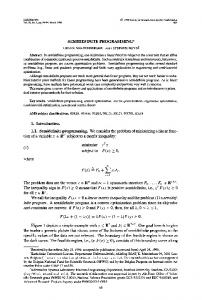
Figure 3. Variation of estimation error with measurement noise 4 anchors, Pure Angle 45 40 35 30
nf=0.05 nf=0.10 nf=0.15 nf=0.20 nf=0.25
20 Error (%R)
Error (%R)
4 anchors, Distance and Angle nf=0.05 nf=0.10 nf=0.15 nf=0.20 nf=0.25
25 20
15
10
15 10
5. Simulation Results
5
5 0.3
For all results, the averages of 25 independent simulations for a particular configuration was computed. Simulations were performed on a networks of 40 nodes randomly placed in a square region of size 1 × 1. Each node was given a random axis orientation between [−π , π ]. The distances between the nodes was calculated. If the distance between 2 nodes i and j was less than a given radio range R, the angle between the axis of i and the direction pointing to node j was computed. If the angle was within field of view, specified by maxang, that is, the maximum angle on either side of the axis at which a node can see other nodes, the angle measurement was included. Otherwise, all other angle measurements were ignored. The angle measurement mechanism is assumed to be omnidirectional(maxang = π ) in our simulations unless otherwise stated. The measured angles were modeled to be noisy by setting θ = θˆ (1 + n f ∗ N(0, 1)) where θ is the measured angle, θˆ is the true value of the angle, n f is a specified constant, and N(0, 1) is a normally distributed random variable. Therefore the noise error in the measurements is modeled as multiplicative and can be varied by changing n f . In order to find relative angles between 2 points as seen from a third point, the measured angles corresponding to the 2 points need to be subtracted, therefore the angle data use in the problem formulation has higher noise variance than the measured angle data. The distance measurements are also modeled to be noisy in ˆ + n f ∗ N(0, 1)) where the same manner. In other words d = d(1 d is the measured distance and dˆ is the actual distance. Figure 3 shows the variation of average estimation error(normalized by the radio range R) when the noise in the angle measurements increases and with different radio ranges. The maxang is set to π , that is, the angle measurement mechanism is assumed to be omnidirectional. 4 anchors are placed near the corners of the square network. There are no more anchors placed in the interior. Figure 4 shows the variation of estimation error when the radio range is increased and with different measurement noises. The advantage of having a higher radio range diminishes beyond a particular value. This can be explained by the fact that beyond a certain radio range, there is enough distance and angle information for the network to be solved. We also disregard some of the redundant information by the random con-
0.4
0.5 Radio Range R
0.6
0.7
0.3
0.4
0.5 Radio Range R
0.6
0.7
Figure 4. Variation of estimation error with Radio Range
4
straint sampling technique in order to keep the number of constraints small enough so that the problem is tractable. In fact for the relaxation proposed, including the extra information may actually deteriorate the solution quality as well,especially for the distance angle case, because with increasing radio range, the multiplicative noise model used implies that the distance measures(corresponding to far away points) will have higher noise. Tuning the radio range such that optimum performance is achieved in terms of computational complexity and accuracy is desirable and it is interesting research question to analyze what such an optimum radio range is for localizing a network and subsequently deriving heuristics to find such a optimum. Overall, the results suggest that when the radio range and the measurements noises are low, that is, we have few measurements but they are reliable, it is preferable to use the distanceangle approach. However, if there are lots of measurements but they have higher uncertainty, it is better to use the pure angle approach. An actual example of this behavior is presented in Figure 5. The anchor positions are shown as blue diamonds, the actual point positions as green circles and the algorithm estimated point positions as red stars. The discrepancies in the positions can be estimated by the offsets between the original and the estimated points as indicated by the solid lines. For Figures 5(a) and 5(b) corresponding to low radio range (R = 0.35) and low noise(n f = 0.05), while the pure angle approach hardly has enough information to solve the network and performs poorly, the distance angle approach provides low error estimation for all the points. For the second case in Figure 5(c),5(d), when the radio range is high(R = 0.7) and noise is high(n f = 0.25), the estimations for quite a few of the points are understandably erroneous owing to the high noise. But the pure angle approach seems to perform slightly better. The effect of a smaller field of view is presented in Figure 6 for varying radio range. For low radio range(R = 0.3) and small field of view (maxang = π /4 − π /3), the accuracy is quite poor for both approaches, greater than 100%R for pure angle
Distance and Angle, R=0.35, nf=0.05
Pure Angle, R=0.35, nf=0.05
0.5
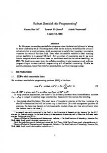
lyzed. Our simulation program is implemented with MATLAB and it uses SEDUMI[7] as the SDP solver. The simulations were performed on a Pentium IV 2.0 GHz and 512 MB RAM PC. Figure 7 illustrates how the solution time increases as the number of points in the network increases. Even with random constraint selection, the solution time seems to increase at a superlinear rate with the number of points. This indicates the necessity of developing a scalable distributed method that was mentioned in Section 4. It is interesting to notice that due the random constraint selection strategy, the running time is almost independent of the radio range. For example, for a network of 40 points, the number of constraints are usually around 480-520. The number of constraints do not change substantially with increasing radio range and therefore the solution time does not change too much with increasing radio range. Furthermore, the pure angle approach uses more constraints and usually takes longer to solve.
0.4
0.2
0
0
−0.2
−0.4
−0.5 −0.5
0
0.5
−0.4
−0.2
(a)
0
0.2
0.4
(b)
Pure Angle, R=0.7, nf=0.25
Distance and Angle, R=0.7, nf=0.25 0.4
0.4
0.3 0.2
0.2
0.1 0
0 −0.1
−0.2
−0.2 −0.3
Radio Range vs Solution Time
−0.4 −0.2
0
0.2
0.4
−0.4
−0.2
(c)
0
0.2
0.4
35
(d)
Solution time(sec)
−0.4
Figure 5. Comparisons in different scenarios
30
Radio Range vs Solution Time 25
R=0.3 R=0.4 R=0.5
Solution time(sec)
−0.4
25 20 15
20
R=0.3 R=0.4 R=0.5
15
10
10 5
case, and 50-80%R for distance angle case. Since distance information is also used in the latter case, the accuracy is better. The lack of more angle information due to limited field of view clearly hurts the accuracy in the pure angle case. Even as the radio range increases, the effect of less angle information goes down, but less dramatically for the pure angle case as for the distance angle case. It is still about 45%R when R = 0.7 for the pure angle case whereas enough information is available in the distance angle case for the error to almost vanish. Pure Angle
60
60 40
50 40 30
10 0.5 Radio Range R
0.6
0.7
0.3
0.4
0.5 Radio Range R
0.6
0.7
Figure 6. Effect of field of view. 40 node network, 4 anchors, nf=0.1 Note that the axis orientations of the points are random. By limiting the field of view and the random axis orientations, it is hard to to establish with certainty if all enough information is available for all the points to be estimated correctly, especially for the pure angle case. Even when points are within radio range of each other, they are not be able to detect each other if they are not in each other’s field of view. As a result, there is very little information for some of the points and they are estimated badly. With higher radio range, this problem can be reduced but the performance is very sensitive because of the random axis orientations. This also suggests that the random constraint selection may need to be fine-tuned in order to include more constraints for the points that appear to have very little information to begin with. The number of constraints and solution time was also ana-
70
30
40
50 60 Number of points
70
[1] Pratik Biswas and Yinyu Ye. A distributed method for solving semidefinite programs arising from ad hoc wireless sensor network localization. Technical report, Dept of Management Science and Engineering, Stanford University, October 2003. [2] Pratik Biswas and Yinyu Ye. Semidefinite programming for ad hoc wireless sensor network localization. In Proceedings of the third international symposium on Information processing in sensor networks, pages 46–54. ACM Press, 2004. [3] Stephen Boyd, Laurent El Ghaoui, Eric Feron, and Venkataramanan Balakrishnan. Linear Matrix Inequalities in System and Control Theory. SIAM., 1994. [4] Lance Doherty, Laurent El Ghaoui, and Kristofer S. J Pister. Convex position estimation in wireless sensor networks. In Proceedings of IEEE Infocom, pages 1655 –1663, Anchorage, Alaska, April 2001. [5] Tzu-Chen Liang, Ta-Chung Wang, and Yinyu Ye. A gradient search method to round the semidefinite programming relaxation solution for ad hoc wireless sensor network localization. Technical report, Dept of Management Science and Engineering, Stanford University, August 2004. [6] Dragos Niculescu and Badri Nath. Ad hoc positioning system (APS) using AoA. In INFOCOM, San Francisco, CA., 2003. [7] Jos F. Sturm. Using SeDuMi 1.02, a MATLAB toolbox for optimization over symmetric cones. Optimization Methods and Software, 11 & 12:625–633, 1999.
20
0.4
50 60 Number of points
References
20 0.3
40
Figure 7. Solution times vs. Number of points
maxang=pi/4 maxang=pi/3 maxang=pi/2 maxang=pi
70
Error (%R)
Error (%R)
80
30
Distance and Angle maxang=pi/4 maxang=pi/3 maxang=pi/2 maxang=pi
100
5
5