Low-Complexity Blind Equalization for OFDM ... - Caltech Authors

1

Low-Complexity Blind Equalization for OFDM Systems with General Constellations Tareq Y. Al-Naffouri, Member, IEEE, Ala’ A. Dahman, Muhammad S. Sohail, Weiyu Xu, Member, IEEE, and Babak Hassibi, Member, IEEE

Abstract This paper proposes a low-complexity algorithm for blind equalization of data in orthogonal frequency division multiplexing (OFDM)-based wireless systems with general constellations. The proposed algorithm is able to recover the data even when the channel changes on a symbol-by-symbol basis, making it suitable for fast fading channels. The proposed algorithm does not require any statistical information about the channel and thus does not suffer from latency normally associated with blind methods. We also demonstrate how to reduce the complexity of the algorithm, which becomes especially low at high signal-to-noise ratio (SNR). Specifically, we show that in the high SNR regime, the number of operations is of the order O(LN ), where L is the cyclic prefix length and N is the total number of subcarriers. Simulation results confirm the favorable performance of our algorithm. Index Terms Channel estimation, maximum a posteriori detection, maximum-likelihood detection, OFDM and recursive least squares.

I. I NTRODUCTION ODERN wireless communication systems are expected to meet ever increasing demands for high data rates. A major hindrance for such high data rate systems is multipath fading. Due to its robustness to multipath fading orthogonal frequency division multiplexing (OFDM) has been incorporated in many existing standards (e.g., IEEE 802.11, IEEE 802.16, DAB, DVB, HyperLAN, ADSL etc.) and is also a candidate for future wireless standards (e.g., IEEE 802.20). All current standards use pilot symbols to obtain channel state information (needed to perform coherent data detection). This reduces the bandwidth available for data transmission, e.g., the IEEE 802.11n standard uses 4 subcarriers (7.1% of the available bandwidth) for pilots of the 56 subcarriers available for transmission. Blind equalization methods are advantageous as they do not require regular training/pilot symbols, thus freeing up valuable bandwidth. There are several works in the literature on blind channel estimation and equalization. A brief classification of these papers based on a few commonly used constraints/assumptions is given in Table I (note that this list is not exhaustive). Broadly speaking, the literature on blind channel estimation can be classified into maximum-likelihood (ML) methods and non-ML methods. The non-ML methods include approaches based on subspace techniques [1]-[10], second-order statistics [11], [12], [13], Cholesky factorization [14], iterative methods [15], virtual carriers [16], real signal characteristics [17] and linear precoding [12], [18]. Subspace-based methods [1]-[5], and [7]-[10] generally have lower complexity, but suffer from slow convergence as they require many OFDM symbols to provide an accurate estimate of the channel autocorrelation matrix. Blind methods based on second-order statistics [11]-[13] also require the channel to be strictly stationary over several OFDM blocks. More often than not, this condition is not fulfilled in wireless scenarios (e.g., in WLAN and fixed wireless applications). Methods based on Cholesky factorization [14] and iterative techniques [15] suffer from high computational complexity. Several ML-based blind methods have been proposed in the literature [19]-[35] and [37]. Although these methods incur higher computational costs, their superior performance and faster convergence are very attractive. These characteristics make this class of algorithms suitable for block fading scenarios with short channel coherence times. Usually, suboptimal approximations are used to reduce the computational complexity of ML-based methods. Although these methods reduce the complexity of the exhaustive ML search, they still incur significantly high computational costa. Some methods like [21], [23], [24] are sensitive to initialization parameters, whereas others work only for specific constellations (see Table I). A few ML-based algorithms allow the channel to change on a symbol-by-symbol basis (e.g., [26], [37]), although these algorithms are only able to deal with constant modulus constellations. To the best of our knowledge, no blind algorithm in the literature is able to deal with channels that change from one OFDM symbol to another when the data symbols are drawn from a general constellation. We therefore present an equalization algorithm with the following key features:

M

This work was supported by a grant from the Deanship of Scientific Research (DSR) at King Fahd University of Petroleum & Minerals (KFUPM) under project No. FT111004. T. Y. Al-Naffouri, A. A. Dahman and M. S. Sohail are with the Electrical Engineering Department, KFUPM, Dhahran, Saudi Arabia. T. Y. AlNaffouri is also with the King Abdullah University of Science and Technology (KAUST), Thuwal, Saudi Arabia (e-mail: [email protected], [email protected], [email protected]). W. Xu is with Department of Electrical and Computer Engineering, University of Iowa, Iowa City, IA (e-mail: [email protected]). B. Hassibi is with Department of Electrical Engineering, California Institute of Technology, Pasadena, CA (e-mail: [email protected]).

2

TABLE I L ITERATURE C LASSIFICATION Constraint Channel constant over M symbols, M >1

Uses pilots to resolve phase ambiguity

Constant modulus constellation

Limited by [1], [2], [3], [5], [6], [7], [9], [10], [11], [12], [13], [14], [15], [17], [18], [20], [16], [21], [24], [27], [28] [1], [5], [9], [10], [11], [14], [15], [16], [18], [20], [21], [28], [25], [26], [37] [2], [3], [6], [9], [12], [13], [15], [16], [20], [21], [24], [26], [27], [36], [37]

Not limited by

[26], [37]

[36]

[1], [5], [7], [11], [14] [17], [19], [28]

1) works with an arbitrary constellation; 2) deals with channels that change from one symbol to the next; 3) assumes no statistical information about the channel. Moreover, we propose a low-complexity implementation of the algorithm by utilizing the special structure of the partial fast Fourier transform (FFT) matrices and show that the complexity becomes especially low in the high SNR regime. The remainder of this paper is organized as follows. Section II describes the system model and Section III describes the proposed blind equalization algorithm. Section IV presents an approximate method to reduce the computational complexity of the algorithm, whereas Section V evaluates this complexity in the high SNR regime. Section VI presents the simulation results and Section VII offers concluding remarks. A. Notation We denote scalars with lower-case letters, x, vectors with lower-case boldface letters, x, whereas the individual entries of a vector, h, are denoted as h(l). Upper case boldface letters, X, represent matrices whereas calligraphic notation, X , is reserved ˆ is an estimate of h. (.)T for vectors in the frequency domain. A hat over a variable indicates an estimate of the variable, e.g., h H and (.) denote the transpose and Hermitian operations, whereas the notation ⊙ stands for element-by-element multiplication. 2π The discrete Fourier transform (DFT) matrix is denoted by Q and defined as ql,k = e−j N (l−1)(k−1) with k, l = 1, 2, · · · , N (N is the number of subcarriers in the OFDM symbol), whereas the inverse DFT (IDFT) is denoted as QH . The notation ∆ ∥a∥2B represents the weighted norm defined as ∥a∥2B = aH Ba for some vector a and matrix B. II. S YSTEM M ODEL Consider an OFDM system where all the N available subcarriers are modulated by data symbols chosen from an arbitrary constellation. The frequency-domain OFDM symbol X , of size N ×1, undergoes an IDFT operation to produce the time-domain symbol x, i.e., √ x = N QH X . (1) The transmitter then appends a length L cyclic prefix (CP) to x and transmits it over the channel. The channel h, of maximum length L + 1 < N , is assumed to be constant for the duration of a single OFDM symbol, but could change from one symbol to the next. The received signal is a convolution of the transmitted signal with the channel observed in additive white circularly symmetric Gaussian noise, n ∼ N (0, I). The CP converts the linear convolution relationship to circular convolution, which, in the frequency domain, reduces to an element-by-element operation. Discarding the CP, the frequency-domain received symbol is given by √ (2) Y = ρ H ⊙ X + N, where ρ is the SNR and Y, H, X ,N , are the N -point DFTs of y, h, x, and additive noise, n, respectively, i.e., [ ] 1 1 1 h H=Q , X = √ Qx, N = √ Qn, and Y = √ Qy. 0 N N N

(3)

Note that h is zero padded before taking its N -point DFT. Let AH consist of first L + 1 columns of Q (i.e., A consists of first L + 1 rows of QH ). Then H = AH h and h = AH.

(4)

3

This allows us to rewrite (2) as Y=

√

ρ diag(X )AH h + N .

(5)

III. T HE B LIND E QUALIZATION A PPROACH Consider the input/output equation (5), which in its element-by-element form reads √ Y(j) = ρ X (j)aH j h + N (j)

(6)

where aj is the jth column of A. The joint ML channel estimation and data detection problem for OFDM channels can be cast as the following minimization problem: √ JM L = min ∥Y − ρ diag(X )AH h∥2 h,X ∈ΩN

=

=

N ∑

min

h,X ∈ΩN

|Y(i) −

i=1  i ∑

min



h,X ∈ΩN

√

|Y(j) −

2 ρ X (i)aH i h|

√

N ∑

2 ρ X (j)aH j h| +

j=1

|Y(j) −

√

2 ρ X (j)aH j h|

j=i+1

  

(7)

where ΩN denotes the set of all possible N −dimensional signal vectors. Let us consider a partial data sequence, X (i) , up to the time index i, i.e.,1 X (i) = [X (1) X (2) · · · X (i)]T and define MX(i) as the corresponding cost function, i.e., MX(i) = min ∥Y (i) −

√

h

2 ρ diag(X (i) )AH (i) h∥ ,

(8)

H where AH (i) consists of the first i rows of A . In the following, we pursue the idea for blind equalization of single-input multiple-output systems first inspired by [19]. Let R be the optimal value for the objective function (7) (below, we show how to determine R in Section III-B). If MX(i) > R, ˆ ML denote the ML ˆ ML , to (7). To prove this, let X ˆ ML and h then X (i) cannot be the first i symbols of the ML solution, X ˆ (i) , satisfies estimates and suppose that our estimate, X

ˆ (i) = X ˆ ML X (i)

(9)

ˆ (i) matches the first i elements of the ML estimate. Then we can write i.e., the estimate X √ R = min ∥Y − ρ diag(X )AH h∥2 h,X ∈ΩN

= ∥Y (i) −

√

N ∑

ˆ ML ∥2 + ˆ ML )AH h ρ diag(X (i) (i)

|Y(j) −

√

ˆ ML |2 ρ Xˆ ML (j)aH j h

j=i+1

= ∥Y (i) −

√

N ∑

ˆ ML ∥2 + ˆ (i) )AH h ρ diag(X (i)

|Y(j) −

√

ˆ ML |2 , ρ Xˆ ML (j)aH j h

(10)

j=i+1

where the last equation follows from (9). Now, clearly √ ˆ ML ∥2 ˆ (i) )AH h ∥Y (i) − ρ diag(X (i)

≥ =

√ ˆ (i) )AH h∥2 min ∥Y (i) − ρ diag(X (i) h √ ˆ 2, ˆ (i) )AH h∥ ∥Y (i) − ρ diag(X (i)

(11) (12)

ˆ is the argument that minimizes the right-hand side (RHS) of (11). Then where h R

= ∥Y (i) −

√

ˆ ML ∥2 + ˆ (i) )AH h ρ diag(X (i)

≥ min ∥Y (i) − h

√

N ∑

√

ˆ ML |2 ρ Xˆ (j)aH j h

j=i+1

ρ

ˆ (i) )AH h∥2 diag(X (i)

= MX(i) . 1 Thus,

|Y(j) −

(13) ∆

for example X (2) = [X (1), X (2)]T and X (N ) = [X (1), · · · , X (N )]T = X .

4

ˆ (i) to correspond to the first i symbols of the ML solution,X ˆ ML , we should have M ˆ < R. Note that the above Thus, for X (i) X(i) ˆ ˆ (i) coincides represents a necessary condition only. If X (i) is such that M ˆ < R, then this does not necessarily mean that X X(i)

ˆ ML . with X (i) This suggests the following method for blind equalization. At each subcarrier frequency, i, make a guess of the new value of ˆ (i) . Estimate h to minimize M ˆ X (i) and use that along with previous estimated values, Xˆ (1), ..., Xˆ (i − 1), to construct X X(i) in (13) and calculate the resulting minimum value of MXˆ(i) . If MXˆ(i) < R, then proceed to i + 1. Otherwise, backtrack in some manner and change the guess for X (j) to some j ≤ i. A problem with this approach is that for i ≤ L + 1, given any choice of Xˆ (i), h can always be chosen by the least-squares method to make MXˆ(i) in (13) equal to zero2 . Then, we will need at least L + 1 pilots; defying the blind nature of our algorithm. Alternatively, our search tree should be at least L + 1 deep before we can obtain a nontrivial (i.e., nonzero) value for MXˆ(i) . An alternative strategy would be to find h using weighted regularized least squares. Specifically, instead of minimizing the objective function, JM L , in (7), we minimize the maximum a posteriori (MAP) objective function, { } √ JM AP = min ∥h∥2R−1 + ∥Y − ρ diag(X )AH h∥2 , (14) h,X ∈ΩN

h

where Rh is the autocorrelation matrix of h (in Section IV, we modify the blind algorithm to avoid the need for channel statistics). Now, the objective function in (14) can be decomposed as               N i   ∑ ∑ √ √ H 2 H 2 2 JM AP = min |Y(j) − ρ X (j)aj h| . (15) ∥h∥R−1 + |Y(j) − ρ X (j)aj h| + h  h,X ∈ΩN    j=i+1 j=1     | {z }       =MX (i)

ˆ (i−1) , the cost function reads Given an estimate of X { } √ ˆ (i−1) )AH h∥2 MXˆ(i−1) = min ∥h∥2R−1 + ∥Y (i−1) − ρ diag(X (i−1)

(16)

with the optimum value (see [38], p. 671) ˆ = √ρ Rh A(i−1) diag(X ˆ H )]−1 Y (i−1) ˆ H )[I + ρ diag(X ˆ (i−1) )AH Rh A(i−1) diag(X h (i−1) (i−1) (i−1)

(17)

h

h

and the corresponding minimum cost (MMSE error) H H −1 ˆ ˆ mmse = [R−1 . h + ρA(i−1) diag(X (i−1) ) diag(X (i−1) )A(i−1) ]

(18)

If we have a guess of X (i), we can update the cost function and obtain MXˆ(i) . In fact, the cost function MXˆ(i) is the same as that of MXˆ(i−1) with the additional observation Y(i) and an additional regressor Xˆ (i)aH i , i.e., 

[ [ ] 2  ]



 H ˆ √ diag(X (i−1) )A(i−1)

Y (i−1)

MXˆ(i) = min ∥h∥2R−1 + h − ρ . (19)

H Y(i) h

 h  Xˆ (i)ai We can thus recursively update the value MXˆ(i) based on MXˆ(i−1) using recursive least squares (RLS) [38], i.e., √ 2 ˆ MXˆ(i) = MXˆ(i−1) + γ(i)|Y(i) − ρ Xˆ (i)aH i hi−1 | ( ) ˆi = h ˆ i−1 + g Y(i) − √ρ Xˆ (i)aH h ˆ i−1 h i i where gi

=

γ(i)

=

√

ρ γ(i)Xˆ (i)H P i−1 ai 1 1 + ρ|Xˆ (i)|2 aH P i−1 ai

(20) (21)

(22) (23)

i

Pi

= P i−1 − ρ γ(i)|Xˆ (i)|2 P i−1 ai aH i P i−1 .

(24)

These recursions apply to all i and are initialized by ˆ −1 = 0. MXˆ(−1) = 0, P −1 = Rh , and h H 2 Since AH is full rank for i ≤ L + 1, diag(X (i) )A(i) is full rank too for each choice of diag(X (i) ) and we will therefore always find some h that (i) will make the objective function in (13) zero (since h has L + 1 degrees of freedom).

5

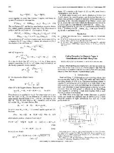
Now, let R be the optimal value for the regularized objective function in (14). If the value R can be estimated, we can restrict ˆ , to the offspring of the partial sequences, X ˆ (i) , that satisfy M ˆ < R. This forms the search of the blind MAP solution, X X(i) the basis for our exact blind algorithm as described below. A. Exact Blind Algorithm In this subsection, we describe the algorithm used to find the MAP solution of the system. The algorithm employs the set of iterations (20)−(24) to update the value of the cost function, MXˆ(i) , which is then compared with the optimal value R. The input parameters for the algorithm are: the received channel output, Y, the initial search radius, r, the modulation constellation3 , Ω, and the 1×N index vector, I. The algorithm is described as follows (the algorithm is also described in the flowchart in Fig. 1) 1) (Initialize) Set i = 1, I(i) = 1 and set Xˆ (i) = Ω(I(i)). 2) (Compare with bound) Compute and store the metric MXˆ(i) . If MXˆ(i) > r, go to 3; else, go to 4; 3) (Backtrack) Find the largest 1 ≤j ≤i such that I(j) < |Ω|. If there exists such j, set i = j and go to 5; else go to 6. ˆ (N ) , 4) (Increment subcarrier) If i < N , set i = i + 1, I(i) = 1, Xˆ (i) = Ω(I(i)) and go to 2; else store the current X update r = MXˆ(N ) and go to 3. 5) (Increment constellation) Set I(i) = I(i) + 1 and Xˆ (i) = Ω(I(i)). Go to 2. ˆ (N ) has been found in Step 4, output it as the MAP solution and terminate; 6) (End/Restart) If a full-length sequence X otherwise, double r and go to 1. The essence of the algorithm is to eliminate any choice of the input that increments the objective function beyond the radius r. When such a case is confronted, the algorithm backtracks (Step 3 then Step 5) to the nearest subcarrier whose alphabet has not been exhausted (the nearest subcarrier will be the current subcarrier if its alphabet set is not exhausted). The other dimension the algorithm works on is properly sizing r; if r is too small such that we are not able to backtrack, the algorithm doubles r (Step 3 then Step 6). If, on the other hand, r is too large such that we reach the last subcarrier too soon, the algorithm reduces r to the most recent value of the objective function (r = MX(N ) ) and backtracks (Step 4 then Step 3). Remark 1: The backtracking algorithm depends heavily on calculating the cost function using (20)-(24). In the constant modulus case, the values of ρ|Xˆ (i)|2 in (23) and (24) become constant (equal to ρ EX ) for all i, and the values of γ(i) and P i become 1 γ(i) = (25) 1 + ρ EX aH i P i−1 ai (26) P i = P i−1 − ρ EX γ(i)P i−1 ai aH i P i−1 , which are independent of the transmitted signal and thus can be calculated offline. Remark 2: The algorithm can also be used for pilot-based standards. In this case, when the algorithm reaches a pilot subcarrier, no backtracking is performed as the value of the data carrier is known perfectly. In the presence of pilots, it is wise to execute the algorithms over the pilot subcarriers first and subsequently to move to the data subcarriers. For equispaced comb-type pilots, (semi)-orthogonality of regressors is still guaranteed. Remark 3: Like all blind algorithms, we use one pilot bit to resolve the sign ambiguity (see references in Table I). B. Determination of ρ, Rh and r Our algorithm depends on ρ, Rh and r, which we need to determine. The receiver can easily estimate ρ by measuring the additive noise variance at its side. As for the channel covariance matrix, Rh , our simulations show that with carrier reordering we can replace Rh with an identity with almost no effect on the performance. This becomes especially true in the high SNR regime. It remains to obtain an initial guess of the search radius, r. To this end, note that if h and X are perfectly known (with h drawn from N (0, Rh ) but known), then √ ξ = ∥h∥2R−1 + ∥Y − ρ diag(X )AH h∥2 (27) h

is a chi-square random variable with k = 2(N + L + 1) degrees of freedom4 . Thus, the search radius should be chosen such that P (ξ > r) ≤ ϵ, where P (ξ > r) = 1 − F (r; k), and where F (r; k) is the cumulative distribution function of the chi-square random variable given by γ(k/2, r/2) . (28) F (r; k) = Γ(k/2) 3 Examples of the modulation constellation Ω are 4-QAM and 16-QAM. We use |Ω| to denote the constellation size and Ω(k) for the kth constellation point. For example, in 4-QAM |Ω| = 4 and Ω(1), · · · , Ω(4) are the four constellation points of 4-QAM. The indicator I(i) refers to the last constellation point visited by our search algorithm at the ith subcarrier. 4 The first term on the RHS has 2(L + 1) degrees of freedom as h is Gaussian distributed whereas the second term has 2N degrees of freedom as √ Y − ρ diag(X )AH h is simply Gaussian noise.

6

Fig. 1.

Flowchart of the blind algorithm.

Here, γ(k/2, r/2) is the lower incomplete gamma function defined as ∫ r/2 γ(k/2, r/2) = tk/2−1 e−t dt.

(29)

0

Under this initial radius, we guarantee finding the MAP solution with a probability of at least 1 − ϵ. In case a solution is not found, the algorithm doubles the value of r and starts over. This process continues until a solution is found. For example, when N = 64, L = 15 and ϵ = 0.01, the value of r should be set to 204. IV. A N A PPROXIMATE B LIND E QUALIZATION M ETHOD There are two main sources for the complexity of the exact blind algorithm introduced in Section III: 1) Calculating P i : the second step of the blind algorithm requires updating the metric MXˆ(N ) . This metric depends heavily on operations involving the (L + 1) × (L + 1) matrix, P i , which is the most computationally expansive (see Table II for estimates of the computational complexity of the RLS). 2) Backtracking: When the condition MXˆ(i) ≤ r is not satisfied, we need to backtrack and pursue another branch of the search tree. This represents a major source of complexity. In the following, we show how we can avoid calculating P i all together. We postpone the issue of backtracking to Section V. A. Avoiding P i Note that in the RLS recursions (20)−(24), P i is always multiplied by ai . We consider how this changes if we set P −1 = I H and assume that the ai is orthogonal (for i = 1, ..., N ) or, in particular, if we assume that aH i ai+1 = ai ai+2 = 0. With these assumptions we note that 1 1 (30) γ(0) = = H 2 ˆ ˆ 1 + ρ |X (0)| a P −1 a0 1 + ρ |X (0)|2 (L + 1) 0

7

TABLE II E STIMATED COMPUTATIONAL COST PER ITERATION OF THE RLS

ALGORITHM

Term

×

+

ˆ ρ Xˆ (i)aH i hi−1 √ 2 ˆ |Y(i) − ρ Xˆ (i)aH i hi−1 | ρ γ(i) MXˆ (i) ˆi h P i−1 ai gi aH i P i−1 ai γ(i) aH i P i−1 Pi Total per iteration

2L + 2 1 1 1

L 1

L+2 L2 + 2L + 1 L+3 L+1 3 L2 + 2L + 1 L2 + 2L + 2 3L2 + 11L + 17

L+1 L2 + L

√

÷

1 1

L 1 L2 + L L2 + 2L + 1 2L2 + 5L + 4

1

1

3

i.e., γ(0) is independent of P −1 . We also note that P 0 a1

= P −1 a1 − ρ γ(0)|Xˆ (0)|2 P −1 a0 aH 0 P −1 a1 2 H ˆ = a1 − ρ γ(0)|X (0)| a0 a0 a1 = a1 .

(31)

For a similar reason, From (31), it is also easy to conclude that γ(1) =

P 0 a2 = a2 .

(32)

1 ˆ 1 + ρ |X (1)|2 (L + 1)

(33)

i.e., γ(1) is independent of P 0 . Also, from (31) and (32), it follows that P i ai+1 = ai+1 and P i ai+2 = ai+2 . We now investigate what happens to P i+1 : P i+1 ai+2

= P i ai+2 − ρ γ(i + 1)|Xˆ (i + 1)|2 P i ai+1 aH i+1 P i ai+2 2 H ˆ = ai+2 − ρ γ(i + 1)|X (i + 1)| ai+1 ai+1 ai+2 = ai+2 .

(34)

Similarly, P i+1 ai+3 = ai+3 .

(35)

Thus, by induction, we see that each occurrence of P i ai in the recursion set (20)-(23) can be replaced with ai . This allows us to discard (24), i.e., √ 2 ˆ MXˆ(i) = MXˆ(i−1) + γ(i)|Y(i) − ρ Xˆ (i)aH (36) i hi−1 | ( ) ˆi = h ˆ i−1 + g Y(i) − √ρ Xˆ (i)aH h ˆ h (37) i i i−1 , where gi

=

γ(i)

=

√

ρ γ(i)Xˆ (i)H ai 1 . ˆ 1 + ρ |X (i)|2 (L + 1)

(38) (39)

Thus, the approximate blind RLS algorithm is effectively running at least mean square (LMS) complexity. Table II summarizes the computational complexity incurred in the RLS calculation. B. Avoiding P i with Carrier Reordering The above reduction in the complexity is based on two assumptions. The first assumption is to set P −1 = I (instead of Rh ) and the second is to assume that the consecutive ai s are orthogonal. Note that the ai s are columns of A, i.e., they are partial FFT vectors. As such, strictly speaking, they are not orthogonal. Notice, however, that for i ̸= i′ , aH i a i′ =

L ∑ k=0

2π

′

e(j N (i−i )k) ,

(40)

8

TABLE III E STIMATED COMPUTATIONAL COST PER ITERATION OF THE RLS Term √ ˆ ˆ ρ X (i)aH i hi−1 √ 2 ˆ |Y(i) − ρ Xˆ (i)aH i hi−1 | ρ γ(i) MXˆ (i) ˆi h γ(i) Total per iteration

ALGORITHM WITH

×

+

2L + 2 1 1 1

L 1

L+2 3 4L + 13

L+1 1 2L + 4

C ARRIER R EORDERING

÷

1 1 1 1 3

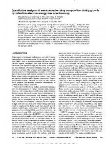
which after straightforward manipulation can be shown to be { ′ L + 1,′ L+1 (i = i ) H . |ai ai′ | = sin(π(i−i ) ) 1 N ̸ i′ ) L+1 sin(π(i−i′ ) 1 ) , (i =

(41)

N

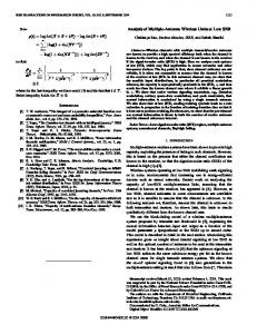
This is a function of (i−i′ ) mod N . Thus, without loss of generality, we can set i′ = 1 and plot this autocorrelation with respect to i. The autocorrelation decays with i as shown in Fig. 2. We can use this observation in implementing our blind RLS algorithm. 1 0.9 0.8

Autocorrelation

0.7 0.6 0.5 0.4 0.3 0.2 0.1 0

0

10

20

30

40

50

60

70

i

Fig. 2.

Autocorrelation vs i for N = 64 and L = 15

Specifically, note that the complete OFDM data are available to us and so we can visit the data subcarriers in any order that we wish. The discussion above shows that the data subcarriers should be visited in the order i, i + ∆, i + 2∆, . . . where ∆ should be chosen as large as possible to make ai , ai+∆ , ai+2∆ , . . . , as orthogonal as possible, but small enough to avoid N revisiting (or looping back to) a neighborhood too early. We found the choice ∆ = L+1 to be a good compromise. From Fig. 2, which plots (41) for N = 64 and L = 15, columns 1, 5, 9, 13, 17, 21, . . . , 61 are orthogonal to each other and so are columns 2, 6, 10, 14, 18, . . . , 62. If the vectors are visited in the following order 1, 5, 9, 13, 17, 21, . . . , 61, 2, 6, 10, 14, 18, . . . , 62, . . ., then we have a consecutive set of vectors that are orthogonal. The only exception is in going from column 61 to 2. These two columns are not really orthogonal but are nearly orthogonal (the correlation of columns 1 and 61 is zero, so the correlation of 61 with 2 should be very small since the correlation function is continuous as shown in Fig. 2). In general, we choose N and visit the columns in the order i + ∆, i + 2∆, . . . , i + L∆, i = 1, . . . , ∆ − 1. ∆ = L+1 Our simulation results show that the bit-error rate (BER) we get with exact calculation of P i and that obtained when we set P −1 = I with subcarrier reordering are almost the same. Table III gives the computational complexity incurred in the RLS calculation when subcarrier reordering is used (i.e., free from P i calculation). Note that with subcarrier reordering, the new version of the RLS runs without the need to use the power delay profile statistics, which relieves us from the need to provide this information.

9

V. C OMPUTATIONAL C OMPLEXITY IN THE H IGH SNR R EGIME In this section, we study the other source of complexity (backtracking) and show that there is almost no backtracking5 in the high SNR regime. To this end, consider the behavior of the algorithm when processing the ith subcarrier. There are |Ω| different alphabets to choose from at this subcarrier and a similar number of possibilities at the preceding i − 1 subcarriers, ¯ (i) and one correct sequence X ˆ (i) . The best case scenario is to have only creating a total of |Ω|i − 1 incorrect sequences X one sequence that satisfies MX¯(i) ≤ r in which case there would be only one node to visit. The worst case is having to visit the remaining |Ω|i − 1 wrong nodes before reaching the true sequence (visiting of nodes will happen through backtracking); this latter case is equivalent to the exhaustive search scenario (i.e., all possible sequences satisfy MX¯(i) ≤ r). Thus, if we let Ci denote the expected number of nodes visited at the ith subcarrier, then, from the above we can write Ci ≤ 1 + (|Ω|i − 1)Pi

(42)

¯ (i) ̸= X ˆ (i) , has a cost less than r. We will where Pi is the maximum probability that an erroneous sequence of symbols, X show that this probability becomes negligibly small at high SNR values. Recall that √ ˆ (i) )AH h + N (i) (43) Y (i) = ρ diag(X (i) where N (i) denotes the first i symbols of N . Note that (43) can be written as [ ][ h ] √ H ˆ Y (i) = . ρ diag(X (i) )A(i) I N (i)

(44)

We first prove our claim for the least squares (LS) cost and then show how the MAP cost reduces to the LS cost for high SNR. A. LS cost ¯ (i) ̸= X ˆ (i) . The LS estimate of h is found by minimizing the Suppose we have an erroneous sequence of symbols, X objective function } { √ 2 h∥ (45) JLS = min ∥Y (i) − ρ diag(X (i) )AH (i) h,X ∈ΩN

and the solution of h is (see [38], Chapter 12, pp. 664) ˆ = [A(i) diag(X ˆ H )diag(X ˆ (i) )AH ]−1 √ρ A(i) diag(X ˆ H )Y (i) . h (i) (i) (i)

(46)

The cost associated with the LS solution is given by (see [38], p. 663) ( ) ( )−1 √ √ ¯ (i) )AH √ρ A(i) diag(X ¯ (i) )H √ρ diag(X ¯ (i) )AH ¯ H ) Y (i) MX¯(i) = Y H ρ diag(X ρA(i) diag(X (i) I − (i) (i) (i) ( ( )−1 ) ¯ (i) )AH ρ A(i) |diag(X ¯ (i) )|2 AH ¯ H ) Y (i) = YH I − ρ diag( X A diag( X (i) (i) (i) (i) (i) ( ρ ) H = Y (i) I − D Y (i) ρ ( ) H MX¯(i) = Y (i) I − D Y (i) (47) where

( )−1 ¯ (i) )AH A(i) |diag(X ¯ (i) )|2 AH ¯ H ). D = diag(X A(i) diag(X (i) (i) (i)

(48)

¯ (i) satisfies MX¯ ≤ r thus reads The probability that the sequence X (i) Pi Pi

= Pr(MX¯(i) ≤ r) ( ) ( ) = Pr Y H I − D Y ≤ r . (i) (i)

In the strict sense of the word, backtracking means visiting Step 3 in our algorithm. Substituting (44) in (49) yields ) (([ [ ]) ]H h h ≤r Pi = Pr G(i) N (i) N (i)

(49)

(50)

5 The term ”backtracking” refers to the case when the algorithm is currently at a subcarrier i and it has to change the estimate of the data symbol at some subcarrier j < i. On the other hand, sweeping the constellation points at the subcarrier to find the first one that satisfies MX(i) ≤ r is not considered backtracking.

10

[

where G(i) =

√

] [ ˆH ) √ ρ A(i) diag(X ˆ (i) )AH (i) [I − D] ρ diag(X (i) I

ˆ (i) )AH . Then G(i) can be written as Let B = diag(X (i) [ ρ B H [I − D] B G(i) = I [I − D] B which in compact form can be expressed as

[

G(i)

ρE = EH 2

B H [I − D] I I [I − D] I

] I .

(51)

]

] E2 . E3

Using the Chernoff bound on the RHS of (50) can be bounded in the following way: [ ( [ ]H [ ]) ] h h µr G(i) Pi ≤ e E exp −µ . N (i) N (i) ] h ∼ N (0, Σ(i) ) N (i)

(52)

(53)

(54)

[

Noting that

with Σ(i) = we express (54) as ∫ Pi

≤ ∫

× = ∫ =

(

[

h exp −µ N (i)

]H

[ G(i)

[ Rh 0

h N (i)

] 0 , Ii

(55)

(56)

]) ( [ ]H [ ]) h h exp − Σ(i) dhdN (i) N (i) N (i)

e−µr π (L+i+1) ( [ ]H [ ]) h h (Σ(i) + µG(i) ) dhdN (i) exp − N (i) N (i) e−µr π (L+i+1) ) ( [ ] h 2 exp − dhdN (i) N (i) (Σ +µG ) (i)

(i)

. (57) e−µr π (L+i+1) Note that the numerator in (57) is a multi-variate complex Gaussian integral. Recall that an n-dimensional complex Gaussian integral has the solution (see [19]) ∫ ( ) πn 2 exp − ||x||W dx = . (58) det(W ) This allows us to simplify (57) as Pi ≤

eµr . det(Σ(i) + µG(i) )

(59)

Next, we show that Pi → 0 as ρ → ∞. To show this, we just need to show that the largest eigenvalue of the term in the denominator, Σ(i) + µG(i) , goes to infinity as ρ → ∞. ˆ H )[I − D]diag(X ˆ (i) )AH be a (L + 1) × (L + 1) matrix. Then, for any sequence X ˆ (i) , Lemma 1: Let E = A(i) diag(X (i) (i) E has a positive maximum eigenvalue, λmax , and a corresponding unit-norm eigenvector v of size (L + 1) × 1. Proof: Recall that ( )−1 ¯ (i) )AH A(i) diag(X ¯ H )diag(X ¯ (i) )AH ¯H ) D = diag(X A(i) diag(X (60) (i) (i) (i) (i) ¯ (i) )AH . Then we can write the above equation as and let F = diag(X (i) ( )−1 D = F F HF FH = FF†

(61)

11

( )−1 where F † = F H F F H is the Moore-Penrose pseudo-inverse6 (see [41], p. 422). Therefore, D is an idempotent matrix with eigenvalues equal to either 0 or 1 [40] and hence, [I − D] is also a positive semi-definite idempotent matrix. Note also that the matrix E in (53) can be written as E

=

ˆ H )[I − D]diag(X ˆ (i) )AH A(i) diag(X (i) (i)

=

B H [I − D]B

(62)

and zH Ez = zH B H [I − D]Bz = (Bz)H [I − D](Bz) ≥ 0

(63)

and so E is Hermitian and positive semi-definite. Let U = [u1 u2 · · · uL+1 ] be a (L + 1) × (L + 1) unitary matrix where ui is the ith eigenvector. Then, E = U ΛU H , where Λ is a diagonal matrix containing ordered eigenvalues of E such that λ1 ≥ λ2 ≥ · · · ≥ λL+1 . Let z = U H v, the maximum eigenvalue of E is given as max vH Ev

||v||2 =1

= = ≤

max zH Λz

(64)

||z||2 =1

max

||z||2 =1

L+1 ∑

λi |zi |2

i=1 L+1 ∑

max λ1

||z||2 =1

|zi |2

(65)

(66)

i=1

≤ λ1 = λmax .

(67)

The equality is attained when v is the eigenvector of λmax . Lemma 2: Given that E has a positive maximum eigenvalue λmax with a corresponding unit-norm vector, v, of size (L + 1) × 1, then the maximum eigenvalue of G(i) in (52) is lower bounded by wH G(i) w = ρ λmax where [ ] v(L+1)×1 w= . (68) 0i×1 Proof: From Lemma 1, the largest eigenvalue of E is λmax . It follows that the largest eigenvalue of ρE is ρλmax . Let λ′max be the largest eigenvalue of G(i) . From (53), we can see that ρE is a principal sub-matrix of G(i) (see [41], p. 494) and thus λ′max ≥ ρλmax (69) i.e., the largest eigenvalue of the principal sub-matrix ρE is smaller than or equal to the largest eigenvalue of G(i) (see [41], pp. 551-552). Thus, ρλmax is a lower bound on the largest eigenvalue of G(i) . Note that Σi is positive definite as it is a covariance matrix. Hence, it will have positive eigenvalues. From Lemma 2, the maximum eigenvalue of G(i) , λ′max → ∞ as ρ → ∞. Thus, the denominator in (59) grows to infinity in the limit ρ → ∞ and lim Pi → 0. (70) ρ→∞

From (42) and (70), we have lim Ci

≤ 1 + (|Ω|i − 1) lim Pi

(71)

lim Ci

≤ 1.

(72)

ρ→∞ ρ→∞

ρ→∞

B. MAP cost ¯ (i) ̸= X ˆ (i) is given as (see [38], p. 672) The cost associated with the MAP solution of an erroneous sequence of symbols X ( )−1 H ¯ ¯H MX¯(i) = Y H Y (i) . (73) (i) I + ρ diag(X (i) )A(i) Rh A(i) diag(X (i) ) Mathematically, Pi Pi 6 The

= Pr(MX¯(i) ≤ r) ( ) ( )−1 ¯ (i) )AH Rh A(i) diag(X ¯H ) = Pr Y H I + ρ diag( X Y ≤ r . (i) (i) (i) (i)

columns of F are linearly independent.

(74)

12

TABLE IV T OTAL COMPUTATIONAL COST OF THE ML

BLIND AND TRAINING - BASED ALGORITHMS AT HIGH

Algorithm

×

+

Blind Algorithm

(3L2 + 11L + 17)N

(2L2 + 5L + 4)N

(4L + 13)N

(2L + 4)N

4L2 + 17L + 13

2L2 + 6L + 4

Blind algorithm with carrier reordering Training-based algorithm [39]

SNR

By the matrix inversion lemma, ( )−1 √ ¯ (i) )AH Rh A(i) diag(X ¯H ) I + ρ diag(X (i) (i) [ ]−1 ¯ (i) )AH R−1 + ρ A(i) diag(X ¯ H )diag(X ¯ (i) )AH ¯H ) = I − ρ diag(X A(i) diag(X (i) (i) (i) (i) h ]−1 [1 H H ¯ (i) )AH ¯ ) ¯ (i) )AH ¯ )diag(X = I − diag(X R−1 + A(i) diag(X A(i) diag(X (i) (i) (i) (i) ρ h = I−D where ¯ (i) )AH D = diag(X (i) Thus, (74) can be written as

[1 ρ

H ¯ ¯ R−1 h + A(i) diag(X (i) )diag(X (i) )A(i) H

( ) ( ) H Pi = Pr Y (i) I − D Y (i) ≤ r .

]−1

H

¯ ). A(i) diag(X (i)

(75)

(76) (77)

(78)

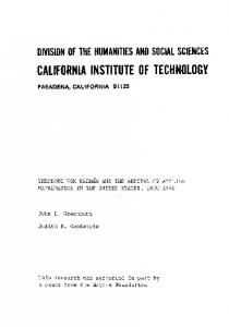
We note that (78) is of the same form as (49). The only difference in the LS and MAP costs is the presence of the term −1 1 ρ Rh in (77). We also note that this term depends on the inverse of the SNR. For low SNR, the inverse term in (77) is always invertible due to the regularization term. At high SNR, the effect of regularization fades and the inverse term in (77) is invertible. At high SNR, i.e., ρ → ∞, ρ1 R−1 h → 0 and D of (76) takes the same form as that of the LS cost leading to (72). Table IV lists the estimated computational cost for our blind algorithm in the high SNR regime. Since there is no backtracking, the total number of iterations is N , which explains our calculations in Table IV. It thus follows that the total number of operations needed for our algorithm is of the order O(LN ) in the high SNR regime. The pilot-based approach for channel estimation needs to invert an (L + 1) × (L + 1) matrix (assuming we need L + 1 pilots to estimate a channel of length L + 1) with a complexity of the order O(L2 ). Since the cyclic prefix is a fixed fraction of the OFDM symbol (L = N/m with m typically set to m = 4 or 8), we see that the complexity of the two approaches becomes comparable in the high SNR regime. VI. S IMULATION R ESULTS We consider an OFDM system with N = 16, or 64 subcarriers and a CP of length L = N4 . The uncoded data symbols are modulated using BPSK, 4-QAM, or 16-QAM. The constructed OFDM signal then passes through a channel of length L + 1, which is assumed to be block fading (i.e., constant over one OFDM symbol but fades independently from one symbol to another) and whose taps follow an exponential decay profile, (E[|h(t)|2 ] = e−0.2t ). A. Bench marking We compare the performance of our algorithm against the following receivers: 1) the subspace-based7 blind receiver of [10]; 2) the sphere decoding based receiver of [28]; 3) a receiver that acquires the channel through training with L + 1 pilots and a priori channel correlation Rh [39]; 4) the ML receiver that acquires data through exhaustive search. The simulations are averaged over 500 Monte-Carlo runs. Fig. 3 compares the BER performance of our algorithm with the aforementioned algorithms for an OFDM system with N = 16 subcarriers and BPSK data symbols. Note in particular that our blind algorithm outperforms both the subspace and sphere decoding algorithms and almost matches the performance of the exhaustive search algorithm for low and high SNR, which confirms the ML nature of the algorithm. Fig. 4, which considers the 4-QAM case, shows the same trends observed for the BPSK case of Fig. 3.

13

0

10

−1

BER

10

−2

10

Subspace algorithm of [10] Sphere decoding [28] Proposed blind algorithm Exhaustive search Channel est. using L+1 pilots and corr. Perfectly known channel

−3

10

−4

10

Fig. 3.

0

5

10

15 SNR(dB)

20

25

30

BER vs SNR for BPSK OFDM over a Rayleigh channel with N = 16 and L = 3 0

10

−1

10

−2

BER

10

−3

10

Subspace algorithm of [10] Sphere decoding [28] Proposed blind algorithm Channel est. using L+1 pilots and corr. Perfectly known channel

−4

10

−5

10

Fig. 4.

0

5

10

15

20 SNR(dB)

25

30

35

40

BER vs SNR for 4-QAM OFDM over a Rayleigh channel with N = 16 and L = 3

Fig. 5 considers a more realistic OFDM symbol length (N = 64), symbols drawn from a 4-QAM constellation and allows the SNR to grow to 45 dB. Our blind algorithm shows no error floor signs, which is characteristic of non-ML methods. Furthermore, the algorithm beats the training-based method and follows closely the performance of the perfect channel knowledge case. Fig. 6 shows the results with N = 64 subcarriers and 16-QAM data symbols for SNR as large as 50 dB. Again, the proposed blind algorithm does not reach an error floor. B. Low-Complexity Variants In this subsection, we investigate the low-complexity variants of our algorithm. Specifically, we consider the performance of the blind algorithm with 1) P i set to I, 2) P i set to I with subcarrier reordering. Fig. 7 exhibits the comparisons for the various algorithms for BPSK and N = 16. Note that with P i set to I arbitrarily, the performance of the blind algorithm deteriorates and the BER reaches an error floor. When we contrast this with the algorithm variant that uses subcarrier reordering as well, we note that the performance of this variant follows closely the performance of the exact blind algorithm. We also note that the BER of both of these algorithms beats that of the sphere decoding algorithm of [28]. The same trends are observed in Fig. 8, which considers the 4-QAM case. 7 The block fading assumption is maintained for all simulations. However, for the subspace blind receiver of [10] to work, the channel needs to stay constant over a sequence of OFDM symbols. For this particular receiver, the channel was kept fixed over 50 OFDM symbols.

14

0

10

−1

10

−2

BER

10

−3

10

−4

10

−5

10

Fig. 5.

10

Channel estimated using L+1 pilots and corr. Proposed Blind Equalization Algorithm Perfectly known channel 15

20

25 30 SNR(dB)

35

40

45

BER vs SNR for 4-QAM OFDM over a Rayleigh channel with N = 64 and L = 15 −2

10

−3

BER

10

−4

10

Channel Estimated using L+1 pilots and Corr. Proposed Blind Equalization Algorithm Perfectly known Channel −5

10

Fig. 6.

30

35

40 SNR(dB)

45

50

BER vs SNR for 16-QAM OFDM over a Rayleigh channel with N = 64 and L = 15

Fig. 9 compares the average runtime of various algorithms as a function of the SNR. We note first that the extreme cases are the training-based receiver and the exhaustive search receiver, both of which are independent of the SNR. The runtime of the proposed algorithm decreases with the SNR and is sandwiched between the run time of the sphere decoding algorithm and that of the subspace algorithm for all values of the SNR8 . We note that in the high SNR regime, our algorithm runs at the same speed as the subspace algorithm. Fig. 10 shows the average runtime of the proposed algorithm with N = 16 for various modulation schemes (BPSK, 4-QAM and 16-QAM). It is clear from the figure that the average runtime decreases considerably at higher SNR values. VII. C ONCLUSION In this paper, we proposed a low-complexity blind algorithm that is able to deal with channels that change on a symbol-bysymbol basis allowing it to deal with fast block fading channels. The algorithm works for general constellations and is able to recover the data from output observations only. Our simulation results demonstrate the favorable performance of the algorithm for general constellations and show that its performance matches the performance of the exhaustive search for small values of N. We have also proposed an approximate blind equalization method (avoiding P i with subcarrier reordering) to reduce the computational complexity. As evident from the simulation results, this approximate method performs quite close to the exact blind algorithm and can work properly without a priori knowledge of the channel statistics. Finally, we studied the complexity of our blind algorithm and showed that it becomes especially low in the high SNR regime. 8 The

runtime of the subspace algorithm is adjusted to account for the fact that it requires the channel to be constant over a block of L + 1 OFDM symbols.

15

0

10

−1

BER

10

−2

10

Subspace algorithm of [10] Sphere decoding [28] Blind Algo. with Pi set to I

−3

10

Blind Algo. with subcarrier reordering Proposed blind algorithm Perfectly known channel

−4

10

Fig. 7.

0

5

10

15 SNR(dB)

20

25

30

Comparison of low-complexity algorithms for BPSK OFDM with N = 16 and L = 3 0

10

−1

10

−2

BER

10

−3

10

Blind Algo. with Pi set to I Blind Algo. with carrier reordering Proposed blind algorithm Channel est. using L+1 pilots and corr. Perfectly known channel

−4

10

−5

10

Fig. 8.

0

5

10

15

20 SNR(dB)

25

30

35

40

Comparison of low-complexity algorithms for 4-QAM OFDM with N = 16 and L = 3

R EFERENCES [1] C. Shin, R. W. Heath, Jr., and E. J. Powers, “Blind channel estimation for MIMO-OFDM systems,” IEEE Trans. Veh. Technol., vol. 56, no. 2, pp. 670-685, Mar. 2007. [2] E. Moulines, P. Duhamel, J. F. Cardoso, and S. Mayrargue, “Subspace methods for the blind identification of multichannel FIR filters,” IEEE Trans. Signal Process., vol. 43, no. 2, pp. 516-525, Feb. 1995. [3] C.-C. Tu and B. Champagne, “Subspace blind MIMO-OFDM channel estimation with short averaging periods: Performance analysis,” in Proc. IEEE Wireless Commun. Netw. Conf., Las Vegas, Neveda, April 2008, pp. 24-29. [4] R. W. Heath Jr. and G. B. Giannakis, “Exploiting input cyclostationarity for blind channel identiffcation in OFDM systems,” IEEE Trans. Sig. Proc., vol. 47, no. 3, pp.848-856, Mar. 1999. [5] B.Su and P.P. Vidyanathan, “Subspace-based blind channel identification for cyclic prefix systems using few received blocks”, IEEE Trans. Signal Process., vol. 55, no. 10, pp. 4979-4993, Oct. 2007. [6] C.-C. Tu and B. Champagne, “Subspace-based blind channel estimation for MIMO-OFDM systems with reduced time averaging,” IEEE Trans. Veh. Technol., vol. 59, no. 3, pp. 1539-1544, Mar. 2010. [7] Y. Zeng and T. S. Ng, “A semi-blind channel estimation method for multiuser multiuser multiantenna OFDM systems,” IEEE Trans. Signal Process., vol. 52, no. 5, pp. 1419-1429, May 2004. [8] X. G. Doukopoulos and G.V. Moustakides, “Blind adaptive channel estimation in OFDM systems,” IEEE Trans. Wireless Commun., vol. 5, no. 7, pp. 1716-1725, Jul. 2006. [9] F. Gao, Y Zeng, A. Nallanathan, T.S. Ng, “Robust subspace blind channel estimation for cyclic prefixed MIMO OFDM systems”, IEEE J. Selet. Areas Commun., vol.26, no.2, pp. 378-388, Feb. 2008. [10] B. Muquet, M. de Courville, and P. Duhamel, “Subspace-based blind and semi-blind channel estimation for OFDM systems,” IEEE Trans. Signal Process., vol. 50, no. 7, pp. 1699-1712, Jul. 2002. [11] H. B¨ olcskei, R. W. Heath, Jr. and A. J. Paulraj, “Blind channel identification and equalization in OFDM-based multiantenna systems,” IEEE Trans. Signal Process., vol. 50, no. 1, pp. 96-109, Jan. 2002. [12] F. Gao and A. Nallanathan, “Blind channel estimation for MIMO OFDM systems via nonredundant linear precoding”IEEE Trans. Signal Process., vol. 55, no. 2, pp. 784-789, Feb. 2007.

16

4

10

Exhaustive search Sphere decoding [28] Proposed exact blind algo. Subspace algorithm of [10] Training based

3

Time(milliseconds)

10

2

10

1

10

0

10

Fig. 9.

0

5

10

15 20 SNR(dB)

25

30

35

Average time comparison for BPSK data symbols with N = 16 and L = 3 7

10

16 QAM 4 QAM BPSK

6

10

5

Time(milliseconds)

10

4

10

3

10

2

10

1

10

0

10

Fig. 10.

0

5

10

15 20 SNR(dB)

25

30

35

Average Time Comparison for our Blind Algorithm for Different Modulation with N = 16 and L = 3

[13] H. Muarkami, “Blind estimation of a fractionally sampled FIR channel for OFDM transmission using residue polynomials”, IEEE Trans. Signal Process., vol. 54, no. 1, pp. 225-234, Jan, 2006. [14] J. Choi and C.C. Lim, “Cholesky factorization based approach for blind FIR channel identification,” IEEE Trans. Signal Process., vol. 56, no. 4, pp. 1730-1735, April 2008. [15] S. A. Banani and R. G. Vaughan, “OFDM with iterative blind channel estimation”, IEEE Trans. on Veh. Technol., vol. 59, no. 9, Nov. 2010. [16] C. Li and S. Roy, “Subspace-based blind channel estimation for OFDM by exploiting virtual carriers,” IEEE Trans. Wireless Commun., vol. 2, no. 1, pp. 141-150, Jan. 2003. [17] F. Gao, A. Nallanathan and C. Tellambura, “Blind channel estimation for cyclic prefixed single-carrier systems by exploiting real symbol characteristics,” IEEE Trans. Veh. Technol., vol. 56, no. 5, pp. 2487-2498, Sep. 2007. [18] A. Petropulu, R. Zhang and R. Lin, “Blind OFDM channel estimation through simple linear precoding,” IEEE Trans. Wireless Commun., vol. 3, no. 2, pp. 647-655, Mar. 2004. [19] W. Xu, M. Stojnic and B. Hassibi, “Low-complexity blind maximum-likelihood detection for SIMO systems with general constellation,” IEEE Int. Conf. on Acoust., Speech and Signal Process. (ICASSP), Las Vegas, Neveda, Apr. 2008, vol. 1, pp. 2817-2820. [20] N. Sarmadi, S. Shahbazpanahi and A. B. Greshman, “Blind channel estimation in orthogonally coded MIMO-OFDM systems”, IEEE Trans. Signal Process., vol. 57, no. 6, pp. 2354-2364, June 2009. [21] W. Ma, B. Vo, T. Davidson, and P. Ching, “Blind ML detection of orthogonal space-time block codes: efficient high-performance implementations,” IEEE Trans. Signal Process., vol. 54, no. 2, pp. 738-751, 2006. [22] E. Larsson, P. Stoica, and J. Li, “On maximum-likelihood detection and decoding for space-time coding systems,” IEEE Trans. Signal Process., vol. 50, no. 4, pp. 937-944, 2002. [23] E. G. Larsson, P. Stoica, and J. Li, “Orthogonal space-time block codes: Maximum likelihood detection for unknown channels and unstructured interferences,” IEEE Trans. Signal Process., vol. 51, no. 2, pp. 362-372, 2003. [24] P. Stoica and G. Ganesan, “Space-time block codes: Trained, blind, and semi-blind detection,” Digital Signal Processing, vol. 13, pp. 93-105, 2003. [25] W.-K. Ma, “Blind ML detection of orthogonal spacetime block codes: Identifiability and code construction,” IEEE Trans. Signal Process., vol. 55, no. 7, pp. 3312-3324, Jul. 2007. [26] T. Y. Al-Naffouri and A. A. Quadeer, “Cyclic prefix based enhanced data recovery in OFDM,” IEEE Trans. on Signal Process., vol. 58, no. 6, pp. 3406-3410, June, 2010.

17

[27] Y. Li, C. Georghiades, and G. Huang, “Iterative maximum likelihood sequence estimation for space-time coded systems,” IEEE Trans. Commun., vol. 49, no. 6, pp. 948-951, 2001. [28] T. Cui and C.Tellambura, “Joint data detection and channel estimation for OFDM systems”, IEEE Trans. Commun.,, vol. 54, no. 4, pp. 670-679, April 2006. [29] A. Gallo, E. Chiavaccini, F. Muratori, and G. Vitetta, “BEM-based SISO detection of orthogonal space-time block codes over frequency flat-fading channels,” IEEE Trans. Wireless Commun., vol. 3, no. 6, pp. 1885-1889, 2004. [30] Y. Hua, “Fast maximum likelihood for blind identification of multiple FIR channels,” IEEE Trans. Signal Process., vol. 44, pp. 661-672, Mar. 1996. [31] B. P. Paris, “Self-adaptive maximum-likelihood sequence estimation,” in Proc. IEEE GLOBECOM, 1993. [32] N. Seshadri, “Joint data and channel estimation using blind trellis search techniques,” IEEE Trans. Commun., vol. 42, pp. 1000-1011, Feb.-Apr. 1994. [33] M. Ghosh and C. L. Weber, “Maximum-likelihood blind equalization,” Optical Engineering, vol. 31, no. 6, pp. 1224-1228, June 1992. [34] S. Talwar, M. Viberg, and A. Paulraj, “Blind estimation of multiple co-channel digital signals using an antenna array,” IEEE Signal Process. Lett., vol. 1, pp. 29-31, Feb. 1994. [35] D. Yellin and B. Porat, “Blind identification of FIR systems excited by discrete-alphabet inputs,” IEEE Trans. Signal Process., vol. 41, pp. 1331-1339, Mar. 1993. [36] M. C. Necker and G. L. St¨ uber, “Totally blind channel estimation for OFDM on fast varying mobile radio channels,” IEEE Trans. Wireless Commun., vol. 3, no. 5, pp. 15141525, Sep. 2004. [37] T.-H. Chang, W.-K. Ma, and C.-Y. Chi, “Maximum-likelihood detection of orthogonal spacetime block coded OFDM in unknown block fading channels,” IEEE Trans. Signal Process., vol. 56, no. 4, pp. 1637-1649, Apr. 2008. [38] Ali H. Sayed, Fundamentals of Adaptive Filtering. John Wiley and Sons, Inc., 2003. [39] T. Y. Al-Naffouri, A. Bahai, and A. Paulraj, “Semi-blind channel identification and equalization in OFDM: an expectation-maximization approach,” in Proc. IEEE Veh. Technol. Conf., Vancouver, Canada, Sep. 2002, vol. 1, pp. 13−17. [40] R. A. Horn, C. R. Johnson, Matrix Analysis, Cambridge University Press, 1990. [41] C. D. Meyer, Matrix Analysis and Applied Linear Algebra, Philadelphia, PA: SIAM, 2000.