Low Complexity Sequential Lossless Coding for

Low Complexity Sequential Lossless Coding for Piecewise Stationary Memoryless Sources  Gil I. Shamiry and Neri Merhav Department of Electrical Engineering Technion - Israel Institute of Technology Technion City, Haifa 32000, ISRAEL Abstract Three strongly sequential, lossless compression schemes, one with linearly growing per-letter computational complexity, and two with xed per-letter complexity, are presented and analyzed for memoryless sources with abruptly changing statistics. The rst method, which improves on Willems' weighting approach, asymptotically achieves a lower bound on the redundancy, and hence is optimal. The second scheme achieves redundancy of O (log N=N ) when the transitions in the statistics are large, and O(log log N= log N ) otherwise. The third approach always p achieves redundancy of O log N=N . Obviously, the two xed complexity approaches can be easily combined to achieve the better redundancy between the two. Simulation results support the analytical bounds derived for all the coding schemes.

Index Terms: Piecewise stationary memoryless source, universal coding, redundancy, min-

imum description length, ideal code length, sequential coding, strongly sequential coding, transition path, weighting, segmentation, change detection, source block code.

 This work was supported by the Israeli Consortium of Ground Stations for Satellite Communications administered

by the S. Neaman Institute for Science & Technology. This work partially summarizes the M.Sc. research work of the rst author. y Gil Shamir is presently at the Department of Electrical Engineering, 275 Fitzpatrick Hall, University of Notre Dame, Notre Dame, IN 46556, U.S.A.

1

1 Introduction Traditional sequential universal lossless source coding schemes are usually designed for classes of stationary sources. Not surprisingly, these schemes may perform poorly when the source is non-stationary, unless some adaptation mechanism is applied. While adaptive schemes such as the dynamic Human code [4], [9], [15], [22] and variations of the sliding-window Lempel-Ziv algorithm [21], [24], [25] have been developed and applied for general non-stationary sources, much less attention has been devoted to systematic, rigorous theoretical development of universal codes for simple classes of non-stationary sources. One example of such a class is that of memoryless sources with piecewise xed letter probabilities [11]-[12], [16]-[19], namely, sources for which the probability mass function (PMF) is subjected to occasional abrupt changes. This model is useful in several application areas, like compression of speech or text retrieved from several sources, edge information in images, and abrupt scene changes in video coding. In this paper, we adopt this simple model of piecewise stationary memoryless source (PSMS ). Neither the source parameters at any stationary segment, nor the transition locations and their number are assumed to be known in advance. One can show that traditional adaptation mechanisms combined with classical compression schemes perform poorly for this class. Dynamic Human coding requires large block length, and thus exponentially large dictionary, in order to approach the entropy even in a stationary segment. Variations of the Lempel-Ziv algorithm require increasing window length, which results in slow convergence to the source entropy. One may use adaptive entropy coding w.r.t. estimated letter probabilities across a sliding window or an exponential one. But such estimates have non-decaying variance, and thus yield poor coding performance. This calls for a dierent approach. First, recall the well-known fact that, ignoring asymptotically negligible integer length constraints, the problem of sequential lossless coding (using e.g., arithmetic coding [7], [8]), is completely equivalent to the problem of sequential probability assignment, where the length function of the code is understood as the negative logarithm of the assigned probability, i.e., the ideal code length . From this point on, we treat the latter problem. To the best of our knowledge, universal coding for the PSMS model was rst investigated by Merhav [11] (see also [12]). Merhav showed that the average universal coding redundancy over all sequences of N letters, drawn by almost any PSMS with C transitions from an alphabet of r letters, is lower bounded by

  RN  (1 ? ") r ?2 1 (C + 1) + C logNN : 2

(1)

This bound was presented as a sum of two terms: The rst term, henceforth referred to as parameter redundancy (PR), corresponds to universality w.r.t. the unknown source parameters within each stationary segment. It consists of 0:5 log N=N bits per symbol for each component of the parameter vector and each stationary segment (see, Rissanen [13]). The second term, henceforth referred to as transition redundancy (TR), corresponds to universality w.r.t. the unknown transition times from one stationary segment to another. This term consists of log N=N bits per symbol for each such transition. In [11], Merhav also demonstrated a universal compression scheme for the PSMS that achieves this lower bound. This scheme employs the method of mixtures in two stages. The rst-stage mixture gives Krichevsky-Tro mov probability estimates [10] for each set of transition times, henceforth referred to as transition path . The second-stage mixture is performed over all possible transition paths. A strongly sequential version of this scheme was also obtained. That is, a scheme that sequentially updates the conditional coding probability of the next symbol given the past, independently of the future and of the horizon N . Merhav's scheme is of linearly increasing per-letter coding complexity, when we assume at most a single transition. It can be generalized to any xed number of transitions, yielding an algorithm of polynomially increasing complexity, and to an exponentially increasing complexity scheme if no assumption of a xed number of transitions is made. Three strongly sequential schemes of smaller, but still increasing complexity, for universal coding of PSMS's were later proposed by Willems [16]-[19]. These schemes are all based on context tree coding [20] combined with arithmetic coding. They all obtain redundancy of at least O (log N=N ), but with coecients larger than the coecient of the lower bound in [11]. Willems implemented two-stage mixtures as described above by constructing suitable state diagrams for the second-stage mixture. The weight of a transition path in the mixture is hence obtained by state transition weights along the path. The rst two schemes ([16]-[18]) take into account all transition paths. In [17] and [18] all transition paths that assume the same most recent transition time are uni ed into one trellis state. This results in linearly increasing per-letter computational complexity, storage complexity of O (N log N ) and redundancy of 0:5 (C + 1) log N=N beyond the lower bound. The second scheme [16], [17] groups transition paths into states according to both the last transition time and the hypothesized number of transitions thus far. The diagram results in more states, each representing less transition paths. This leads to quadratically increasing per-letter complexity and a total redundancy of 0:5 log N=N beyond the bound. The third approach, proposed recently in [19], selectively eliminates states according to the time they were created. This scheme is still of 3





increasing complexity of O (log N ) and achieves per-letter redundancy of O log2 N=N overall. To the best of our knowledge, no xed complexity universal scheme has been obtained for PSMS's. In this paper, we derive, analyze and present simulation results of three new universal strongly sequential data compression schemes for PSMS's based on context tree coding. The rst scheme achieves the lower bound on the redundancy, whereas the two other schemes provide slower decay rate of the redundancy, but have xed complexity (and logarithmic bit storage complexity). The rst scheme is a generalization of Merhav's scheme which uses Willems' linear transition diagram with dierent weights. Similarly as Willems' scheme, it is of linearly increasing per-letter complexity. Unlike all the schemes presented in [11], [16]-[19], for which the number of states grows with time, the last two schemes have xed number of states, and hence can be applied for practical purposes. Although the convergence rate does not meet the bound, it is better than any existing low-complexity scheme for PSMS's. The second scheme combines decisions based on the observed past with a reduced-state transition diagram, using dierent state transition weights than those used by Willems. It uses decisions to eliminate unlikely states in the diagram, thus preserving a xed number of states. This scheme achieves average redundancy of O (log N=N ) for large transitions if the number of stationary segments is upper bounded by some constant S , that depends on the design parameters of the scheme. Otherwise, pointwise redundancy (for any N -tuple) of at most O (log log N= log N ) is obtained. In the third scheme, we partition the data sequence into smaller blocks and encode each one separately.  p Using the optimal block length, we achieve pointwise redundancy of O log N=N . Simulations show that the true redundancies of the last two schemes are even better than the upper bounds obtained. We can easily combine both xed complexity schemes to obtain the better redundancy between  p the two for any sequence. We hence obtain a maximum upper bound of O log N=N , which is better than the currently known O (1= log N ) upper bound of the Lempel-Ziv algorithm. The outline of this paper is as follows. Section 2 contains notation and de nitions. In Section 3 we generalize the analysis for the redundancy of a coding scheme. Section 4 presents the rst scheme of linear per-letter complexity. In Section 5, we describe and analyze the second scheme of decisions and weighting. Section 6 presents the block partitioning scheme along with the analysis of its rate of convergence. Numerical results are presented in Section 7. Finally, in Section 8, we present the summary and conclusions of this work.

4

2 Notation and De nitions Let fP g be a parametric family of memoryless stationary PMF's of vectors whose components take on values in a nite alphabet  of size r. The parameter  designates the r ? 1 dimensional vector of letter probabilities. A string drawn by the source from time instant i to time instant 4 (x ; x ; : : : ; x ; : : : ; x ) be a 4 xN = j (xi; xi+1 ; : : : ; xj ) ; j > i, will be denoted by xji . Let xN1 = 1 2 n N string emitted from an r-ary PMF whose parameter  takes on a particular value 0 from n = 1 to n = t1 ? 1; then  = 1 from n = t1 until n = t2 ? 1, and so on. Finally, from n = tC to n = N ,  is held at C . The vectors fx1 ; : : : ; xt1 ?1 g, fxt1 ; : : : ; xt2 ?1 g ;


; fxtC ; : : : ; xN g will be referred to as stationary segments , and correspondingly, 0 ; 1 ;


; C will be called the segmental parameters . It will be assumed that the dierent segments are statistically independent. The extended vector (0 ; 1 ; : : : ; C ) will be denoted by , and will be referred to as the parameter set . The C dimensional vector, representing the C time instants before which transitions take place, (t1 ; t2 ; : : : ; tC ), will be denoted by T , and referred to as the true transition path . For convenience, 4 1 and t 4 we de ne t0 = C +1 = N + 1. We will assume that the number of transitions C is either xed or is of lower order than the time n. Noting that C is a function of the dimension of the other parameters, the PMF of the PSMS is parameterized by the pair f; T g, and de ned as follows.



C  Y

P xN j ; T =




?

i=0

Pi xti ; : : : ; xti+1 ?1 ;

(2)

where the PMF of each segment is obtained by

?




Pi xti ; : : : ; xti+1 ?1 = =

ti+1 Y?1 n=ti

Y

u2

Pi (xn) ti+1 ?1 (u)

Pi (u)nti

(3)

;

where Pi (xn ) is the probability of the letter xn drawn by Pi , which for simplicity, will be denoted by Pi , and nttii+1 ?1 (u) denotes the number of occurrences of u 2  within the i-th segment. The per-letter average entropy of a PSMS is obtained by 4 1 H (; T ) = N

C X i=0

(ti+1 ? ti ) H (i ) ;

(4)

where H (i ) is the entropy of the i-th segment. Since we assume no prior knowledge of f; T g, we will not be able to assign the true probability of the sequence for a coding scheme. Instead, we will seek a universal sequential probability assignment that will implement a two stage mixture and will serve as the basis for arithmetic 5

coding. The probability assigned to the substring xn by an algorithm A will be denoted by QA (xn ). ?
To enable sequential updating of QA , the conditional probability QA xn j xn?1 de ned by [13] as

   4 QA xn j xn?1 = QA (xn ) =QA xn?1 ;

(5)

must be well de ned. Additionally, in order to enable the use of arithmetic coding, the assigned probability must ful ll the terms described in [20]





QA x1n?1 =

X

xn 2

QA (xn1 ) ; 8x1n?1 2 n?1 ;

(6)

where the probability of the empty string is one by convention. The rst-stage mixture, implemented to obtain the assigned probability, is performed for a given   transition path. The conditional probability assignment Q xN j T 0 given any transition path T 0 =4 (t01; : : : ; t0C ), is recursively de ned using the Krichevsky-Tro mov (KT) empirical estimates [10], that result from mixing the parameter with a Dirichlet(0:5) prior. The KT estimates will be used with relative frequency counts that are reset at every hypothesized transition. Speci cally, the conditional letter probability is de ned as

Q

 4 ntt?0i 1 (u) + 21 t ? 1 0 Xt = u j x1 ; T = (n ? t0 ) + r ; i 2



t0i  t < t0i+1 ; 8u 2 ;

and the probability of an n-tuple is obtained by

?




Q xn1 j T 0 =

n  Y

Q xi j xi1?1 ; T 0



i=1

   = Q x1n?1 j T 0
Q xn j x1n?1 ; T 0 ;

(7)

(8)

where x01 represents the null string, whose probability is one by convention. To implement the second stage mixture, the probability assigned to an N -tuple will be a weighted sum of conditional probability assignments given transition paths. Each probability assumes a dierent path T 0 from a set of paths fT gA , selected by the algorithm A. Each path will be weighted with some weight function WA (T 0 ).

 

QA xN =

X

T 0 2fT gA

 ?
 WA T 0 Q xN j T 0 :

(9)

The weight function must be non-negative for all T 0 and satisfy

X

T 0 2fT gA

?
WA T 0 = 1: 6

(10)

The idea of the coding scheme is to construct a group fT gA that always includes the true   transition set T , or at least a good estimate T^ of T , that induces large values of Q xN j T^ n ^ ^ ^o   ; T , where ^ is de ned by convex and WA T^ . Such an estimate T^ de nes a triplet C; combinations of the true segmental parameters i along each hypothesized segment. The weights of each convex combination are the relative durations of each i within the hypothesized segment of T^ . For example, if T = fN + 1g ; 0 <  < 1, i.e., a single true transition, but we estimate n o no transitions, i.e., T^ = , then ^ = ^0 , where ^0 = 0 + (1 ? ) 1 . We de ne the probability   assignment for an estimated PSMS as Q xN j ^ ; T^ , similarly as in eq. (2).

3 The Redundancy The pointwise redundancy of scheme A for an N -tuple xN is de ned as

N   P x j  ; T 4 1 R xN ; A = N log QA (xN ) ; 

(11)

ignoring negligible integer length constraints. The (expected) N -th order redundancy of scheme A is de ned as h  i 4E (12) RN (A) = f;T g R xN ; A ; where Ef;T g denotes the expectation w.r.t. a given PSMS f; T g. The pointwise redundancy of an N -tuple for a PSMS can be expressed as



R xN ; A















Q xN j T^ Q xN j ^ ; T^ P xN j ; T = N1 log Q (xN ) + N1 log  N ^  + N1 log  N ^ ^  A Q x jT Q x j ; T

(13)

4 R xN ; A + R xN ; A + R xN ; A = p t d

Eq. (13) decomposes the pointwise redundancy into three terms: Rt - transition redundancy (TR), Rp - parameter redundancy (PR), and Rd - decision redundancy (DR). The TR re ects universality w.r.t. the transition path. The PR is the cost of universality w.r.t.  for a given transition set. The DR is the additional redundancy caused by estimation error of the transition path and the segmental parameters it imposes. These terms all depend on the speci c algorithm, but of course, it is the total redundancy that should be compared to the lower bound. Assigning the KT estimate to a stationary segment of length m results in additional r?2 1 log m + O (1) code bits of unnormalized PR for that segment [10], [14], similarly to Rissanen's lower bound.   Hence, using the conditional probability assignment of eqs. (7)-(8) for Q xN j T^ results in extra 7

code length, that is the sum of the additional code bits obtained for each of the segments imposed by T^ . Using the Jensen inequality and normalizing by N , we conclude that the PR is upper bounded by  N  r ? 1  ^  log C^N+1 ^! C Rp x ; A  2 C + 1 N + O N (14) From eq. (9) and the de nition of TR in (13), we obtain that the TR depends on the weight of T^ and is upper bounded by    N  4 1 Q xN j T^ (15) Rt x ; A = N log Q (xN ) A   Q xN j T^ 1 = N log P T 0 2fT gA WA (T 0 ) Q (xN j T 0 )    ? 1 log WA T^ :

N

The inequality holds by de nition of T^ . The DR results from coding more than one true stationary segment as if it were a single stationary block. Assume the block xii++1m of length m contains data drawn by s distributions Pu+1 to Pu+s , and assume this block is coded as if it were drawn by a stationary PMF Q, then Q is de ned as the convex combination of the true distributions, where each PMF Pu+l is weighed by its relative duration in the block. It is easy to show that the contribution to the DR of this block is upper bounded by the entropy of the relative durations vector multiplied by m and normalized by the complete sequence length N . Since the vector consists of s components, we can bound the contribution of this block to the DR by   (16) R xi+m ; A  m log s : d

i+1

N

The DR of an N -tuple is the sum of the contributions of all segments hypothesized by T^ .

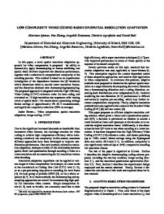
4 An Optimal Linear Per-Letter Complexity Scheme The scheme presented in this section and denoted by W , uses Willems' linear weighting scheme [17], [18] to group transition paths into states in a diagram, but with dierent weight functions, corresponding to the scheme in [11]. It will be shown to achieve the lower bound on the redundancy, as opposed to Willems' scheme. The idea of Willems' linear scheme is to implement the mixture method using a linear transition diagram that contains all possible transition paths, as illustrated in Figure 1. This trellis reduces the exponential complexity and still enables weighting of all transitions paths. A directed path 8

4

3

3

2

2

2

1

1

1

1

n = 1

2

3

4

Figure 1:

linear transition diagram at time instants 1 to 4. A number in a state box denotes the most recent transition point of the state represented by the box. The time is denoted below the graph.

along the diagram represents a transition path. Horizontal move denotes that the source remains in the same stationary segment. An upward move in the graph represents a transition of the source. A box in the diagram represents a state. State sn at time n is de ned as the time instant of the most recent transition within the period 1  t  n. Each state is assigned a weight G (xn1 j sn ) associated with the subsequence xn1 , in order to implement the weighting procedure. The probability assigned to xn1 is the sum of the weights of all states in the diagram at time n. 4 QW (xn1 ) =

n X

sn =1

G (xn1 j sn) :

(17)

We note that by de nition of a state, the diagram will always consist of n states at time n, that form a partition of all transitions paths into n disjoint sets. The weight of a state is recursively de ned by the KT estimates and the transition rules of the trellis. The KT probability of letter xn at state sn is obtained, similarly as in (7), by 4 nsnn?1 (xn ) + 21 : Q ( x n j sn ) = (n ? s ) + r n

2

(18)

The only two possible transitions from state sn at time n to state sn+1 at time n + 1 are the self transition, i.e., sn+1 = sn and sn+1 = n + 1, i.e., transition to the only new state formed at time n + 1 that assumes a source transition between time n and time n + 1. Associated with each such 9

transition, there is a weight Wtr (sn+1 j sn ), where

Wtr (sn+1 = sn j sn) + Wtr (sn+1 = n + 1 j sn) = 1:

(19)

The weight of a state is therefore recursively updated by

8   n?1 > < ; s Pn?1  n?1  n : j=1 Wtr (sn = n j sn?1 = j ) G x1 j sn?1 = j ; sn = n

It is easy to see that the weight assigned to a state by this procedure is a weighted sum of the KT estimates assigned to all transition paths Tn0 of order n that lead to this state,

G (xn1 j sn ) =

X

?
?

Tn0 !sn




W Tn0 Q xn1 j Tn0 ;

(21)

where Tn0 ! sn is the set of all paths leading to sn . The weight W (Tn0 ) is the product of all the transition weights along the path representing Tn0 in the diagram. So far, we have described a general linear scheme as presented in [17], [18]. The transition weights de ned by Willems use the binary KT estimates of the distance from the last transition.

8 > 4< Wtr (sn+1 j sn) = > :

1 2

(n?sn )+1 ; (n?sn )+ 21 (n?sn )+1 ;

sn+1 = n + 1 : sn+1 = sn

(22)

The proposed scheme de nes state transition weights Wtr (sn+1 j sn ), that are dierent from those de ned above. The weights are de ned as follows. For a given " > 0, let: 4 1 ; 1  j < N;  (j ) = j 1+" n 4 X  (j ) ; Cn = j =1

and C1 = Now,

8 > 4< Wtr (sn+1 j sn) = > :

1 X

j =1

 (j ) :

(n) C1 ?Cn?1 ; C1 ?Cn C1 ?Cn?1 ;

(23) (24) (25)

sn+1 = n + 1 : sn+1 = sn

(26)

By eqs. (23)-(26), we assign to each time n; 1  n < N , a distribution over the xed time t; t > n for the probability that the next transition occurs just before time t. The probability of source transition at time n +1 is the weight Wtr (n + 1 j sn), which is selected to decay as n?(1+") , causing additional TR of (1 + ") log n=N if a true transition occurs at that point. We note that the above weights depend on the absolute time, instead of the relative time from the last transition as in 10

(22). This reduces the weight of a transition, and is justi ed by the assumption that the number of transitions is small. This also leads to a computational improvement. First, the self-transition weight can be calculated once using (26) for all self-transitions in eq. (20). Furthermore, eq. (20) for sn = n reduces, using eq. (17), to





G (xn1 j sn = n) = Q (xn j sn )
Wtr (sn = n j sn?1 < n) QW x1n?1 ;

(27)

where Wtr (sn = n j sn?1 < n) is the same for all sn?1 < n. The drawback of the scheme with these weights is that it is computationally more demanding than the scheme with Willems' weights. Willems' weights attain pointwise redundancy higher than the lower bound, presented in (1), C      R xN ; L  r ?2 1 (C + 1) + 3C 2+ 1 logNN + O N ; (28) where L denotes Willems' scheme. The quadratical per-letter complexity scheme does not attain the bound either. The scheme with the proposed weights, on the other hand, attains the lower bound. This is stated in the following theorem.

Theorem 1 The redundancy of the linear weighting scheme with state transition weights as in (26), is upper bounded by

 C     R xN ; W  r ?2 1 (C + 1) + C + " logNN + O N for every N -tuple drawn by any PSMS, for all " > 0. 4 log(log 2j ) , k > 1, and If we let " decay slowly with time, such that "j = log j 1 ; 4 j ?(1+"j ) =  (j ) = j (log 2j )k we have  log N  C log log N   N  r ? 1 : R x ; W  2 (C + 1) + C N + O N

(29)

k

(30) (31)

We conclude this section with the proof of the theorem.

Proof of Theorem 1: It is straightforward that this coding scheme satis es eq. (9) (see e.g. [17]), and weighs all possible transition paths. Therefore, the true path T is always included, and so, Rd = 0 and T^ = T . The PR is upper bounded by (14), with C^ = C , and thus attains the lower bound, as expressed by the rst term of (29). It is thus sucient to show that the TR attains the lower bound as well. We will show that





Rt xN ; W  N1 [(C + ") log N + (C + 1) (1 + ") ? C log "] : 11

(32)

We will rst obtain WW (T ) using (26), and then upper and lower bound the partial sum C1 ? Cn ; 8n : 0  n < N , by approximating the sum by an integral. Finally, we will apply these bounds to the cumulative weight function WW (T ) and upper bound TR by ? log WW (T ) =N . The weight of T is obtained by

WW (T ) =

2 C Y 4

i=0 NY ?1

Wtr (sti = ti j sti?1 = ti?1 )


ti+1 Y?1 j =ti +1

3 Wtr (sj = ti j sj?1 = ti )5

(33)

C W (s = t j t ) Y tr ti i i?1 n=1 i=1 Wtr (sti = ti?1 j ti?1 ) C NY ?1 C ? C 1 n
Y  (ti ? 1) = n=1 C1 ? Cn?1 i=1 C1 ? Cti ?1 C  (t ? 1) CN ?1
Y i = C1 ? : C1 i=1 C1 ? Cti ?1

=

Wtr (sn+1 = sn j sn)


4 1. The rst equality is obtained by taking the transition weights We de ne Wtr (s1 = 1js0 = t?1 ) = along T . The second equality is obtained by multiplication and division by the self-transition weights at points of true source transitions. We use the telescopic property of the rst product to obtain the last equality.

Approximating the in nite sum by an integral, we bound the partial sum C1 ? Cn by 21+" ; 8n  0: 1  C ? C  1 n " " (n + 1) " (n + 1)"

(34)

We note that C1 = C1 ? C0. Finally, we use this bound to upper bound the transition redundancy by the upper bound of eq. (15).



Rt xN ; W



 ? N1 log WW (T ) # "X C 1 C ? C 1 t ? 1 i = N log  (t ? 1) ? log (C1 ? CN ?1 ) + log C1 i i=1 "X C 1+" # 1+" (ti ? 1)1+" 2 2 1 " + log ("N ) + log log  N

 N1

i=1 "X C i=1

"t"i

"

log ti1+"?" + " log N + (C + 1) (1 + ") ? C log "

(35)

#

 N1 [(C + ") log N + (C + 1) (1 + ") ? C log "] :

The last inequality is obtained by taking N as an upper bound on ti . This proves that the TR attains the lower bound, and therefore concludes the proof of the theorem. 12

5 A Decision Weighting Scheme In this section we show that there exists a xed complexity scheme, based on the transition diagram of the linear per-letter complexity scheme, that achieves vanishing redundancy. The redundancy is of the order of the lower bound when the transitions are large. We refer to the new scheme as the decision weighting scheme (DW), and denote it by D. This scheme uses a data-dependent reduced-state transition diagram . It eliminates transition paths with low likelihood and it does not create a new state every time instant. The scheme produces new states every k  1 time instants instead of every instant, in order to reduce the diagram's growth rate. This forms a partition of the data into N=k non-overlapping blocks of length k, and for each block only one state is created. The parameter k is a design parameter, that will be referred to as the block length . In order to keep the number of surviving states (and the computational complexity) xed, we assign to each state s a metric M (s), that determines the likelihood of transition within the block represented by s. States with low metric values are eliminated. The number of high metric surviving states S is the second design parameter of the algorithm. By de nition of the transition diagram, the set of surviving states de nes a set of surviving transition paths, and a transition path that leads to an eliminated state is said to be eliminated and not to exist in the diagram. The state number s represents the block number in which the most recent transition is assumed to have occurred. A state s; s > 1, that estimates transition at any time within the block it represents, is created at the block midpoint. The rst state s = 1 is naturally created at the rst time instant. The metric of a state s is de ned as follows. Let ns (u) be the number of occurrences of the the letter u in block s. The empirical per-letter entropy of the block is obtained by X H (s) = ? ns (u) log ns (u) : (36)

k

u2

k

The empirical entropy of the concatenation of blocks r and s is obtained by X H (r; s) = ? nr (u) 2+k ns (u) log nr (u) 2+k ns (u) : u2

(37)

Now, M (s) is de ned by

M (1) M (s)

4 1 =

4 = H (s ? 1; s + 1) ? 21 H (s ? 1) ? 21 H (s + 1) ; 8s > 1:

13

(38) (39)

M(r)

AAAAAAAA AAAAAAAA AAAAAAAA AAAAAAAA AAAAAAAA AAAAAAAA AAAA AAAAAAAA AAAAAAAAAAAA AAAAAAAA AAAAAAAAAAAAAAAA r-1

M(s)

AAAAAAAA AAAAAAAA AAAAAAAA AAAAAAAA AAAAAAAA AAAAAAAA AAAA AAAAAAAA AAAAAAAAAAAA AAAAAAAA AAAAAAAAAAAAAAAA r

T

AAAAAAAA AAAAAAAA AAAAAAAA AAAAAAAA AAAAAAAA AAAAAAAA AAAA AAAAAAAA AAAAAAAAAAAA AAAAAAAA AAAAAAAAAAAAAAAA

r+1

s-1

s

AAAAAAAA AAAAAAAA AAAAAAAA AAAAAAAA AAAAAAAA AAAAAAAA AAAA AAAAAAAA AAAAAAAAAAAA AAAAAAAA AAAAAAAAAAAAAAAA s+1

k

Figure 2:

block partitioning for DW. The solid line represents the data sequence, that is divided into blocks of length k. True transition occurs at T and can be only estimated at the block midpoint by state s with likelihood M (s), obtained by the empirical data of the two neighboring blocks s ? 1 and s + 1. Another estimated transition is within block r estimated at its midpoint, with likelihood M (r).

The quantity M (s) measures the `distance' between the empirical distributions of blocks s ? 1 and s + 1. If M (s) is large then it is likely that a change has occurred within block s. It is well-known that M (s) serves as asymptotically optimal statistics for testing weather or not two sequences emerged from the same source [6], [23]. If M (s) is large the scheme will assume transition which will be referred to the midpoint of block s by state s in the trellis. Figure 2 illustrates the partitioning mechanism. The metric M (s) is non-negative for all s > 1, even if transition has not occurred. This can cause elimination of s = 1 if its metric had been de ned smaller, even when other transitions have not occurred. Since state s = 1 always represents a transition, we thus de ne its metric to be in nite. The probability assignment scheme can be described by the state diagram shown in Figure 3 for k = 4 and S = 3. The diagram begins when all S high metric states already exist, i.e., in steady state. The boxes in the diagram denote the states, and the numbers in the boxes the block numbers of the most recent transitions assumed by the states. As in the linear scheme, each state is assigned a weight G (xn1 j sn ) associated with the subsequence xn1 . The weight of a state is recursively de ned by the KT estimates and the transition rules shown in the diagram. The KT probability of letter xn at state sn is obtained by 4 nnn?1 (xn ) + 21 ; Q ( x n j sn ) = (n ?  ) + r n

2

(40)

where the time n is the rst time instant after the last transition assumed by sn, which is de ned by 8 > sn = 1 4 < 1; n = : (41) > : b(sn ? 0:5) kc + 1; sn > 1 The transition rules and update procedures at each time point are de ned for three dierent cases as follows: 14

r+1

r+1

r+2

r

r

r

r

r+1

r+1

r+1

r+1

r+2

r+2

r-1

r-1

r-1

r-1

r

r

r

r

r+1

r+1

r-2

r-2

r-2

r-2

r-1

r-1

r-1

r-1

r

r

test r-3 with {r-2,r-1,1,s1,s2} Eliminate r-3

n=m+

r+2

test r-2 with {r-1,r,1,s1,s2} Eliminate r-2

test r-1 with {r,r+1,1,s1,s2} Eliminate s1

s2

s2

s2

s2

s2

s2

s2

s2

s2

s2

s1

s1

s1

s1

s1

s1

s1

s1

r-1

r-1

1

1

1

1

1

1

1

1

1

1

1

2

3

4

5

6

7

8

9

10

Figure 3:

example of DW transition diagram in steady state for k = 4 and S = 3. The diagram starts right after time instant m at the rst point of the r + 1 block. A single new state is created at any block midpoint, and a single low metric state is eliminated at any block partition point. Time instants are denoted below the diagram.

1. At a block midpoint n = b(m + 0:5) kc + 1; m > 0 xed, a new state r is created. The state weights are recursively updated almost as in the linear scheme by

8   n?1 > < ; sn < r W ( s = s j s )
G x j s tr n n ? 1 n ? 1 n ? 1 G (xn1 j sn) = Q (xn j sn)
> Pr?1 ; (42)  n?11  : j=1 Wtr (sn = r j j ) G x1 j sn?1 = j ; sn = r

where the transition weights are obtained by

8 > < 4 Wtr (sn+1 j sn = j ) = > :

(r?j ) C1 ?Cr?j?1 ; C1 ?Cr?j C1 ?Cr?j?1 ;



sn+1 = r : sn+1 = j

(43)



(The weight of a previously eliminated state j is zero G x1n?1 j j = 0 ). We note that the transition weights depend on the relative block number from the last transition instead of the absolute time, as in the linear scheme. The proof of Theorem 2 will be based on this de nition. 2. At the rst point of a new block n = mk +1; m  5 xed, at most a single state i is eliminated into another state j . The weight of i is added into the weight of j , which is the smallest state in the diagram that is still larger than i. Only the self-transition is performed from all other 15

states.

8 > > < 0;  n?1   n?1  sn = i n G (x1 j sn) = Q (xn j sn)
> G x1 j i + G x1 j j ; sn = j : > : G x1n?1 j sn ; otherwise

3. At any other point n there are only self-transitions.



G (xn1 j sn) = Q (xn j sn)
G x1n?1 j sn = sn?1



(44)

(45)

The elimination retains a xed number of states in the diagram. It also ensures that no more than one state of any three consecutive states remain in the diagram. This is done to avoid a situation where a single transition is represented by two or three states. If a transition occurs at the midpoint of block s, all three states s ? 1, s and s + 1 may have large metrics, and we only need to save one of them to represent the transition. We will therefore eliminate the states with the lower metric values among the three. The computation of the metric of state s requires delay of 1:5k time points, to obtain the empirical data of block s + 1. An additional delay of 2k points is required for computation of the metrics of s + 1 and s + 2, that are tested against s. Hence, every new state will exist at least 3:5k time points before it is tested for the rst time. Due to the delay of 3:5k time points between creation and the rst possible elimination of a state, the steady state diagram contains S + 3 states at time points of rst halves of partition blocks and S + 4 states at time points of second halves. The elimination procedure at n = mk + 1 takes three stages of testing the metric of the state s, created at n ? 3:5k. If s ? 1 or s ? 2 exist in the diagram, state s is eliminated, since M (s ? 1)  M (s) or M (s ? 2)  M (s). Otherwise, state s is tested against states s +1 and s +2, and if M (s + 1) > M (s) or M (s + 2) > M (s), s is eliminated. If s passed both tests and there are less than S states, created before n ? 3:5k, no elimination is performed. If there are S such states, the state with the lowest metric among the existing states, created at n ? 3:5k or earlier, is eliminated. A state is always eliminated by adding its weight into the weight of the closest newer state. This strategy minimizes the DR in case a true transition is eliminated by replacing it by the closest hypothesized transition point, still existing in the diagram. The probability assigned to the subsequence xn is obtained, as in the linear scheme, by the sum of the weights of all states that exist in the diagram at time instant n.

QD (xn1 ) =

X sn

16

G (xn1 j sn) ;

(46)

P

where the notation sn represents a sum over all states existing in the diagram at time instant n. In contrast to the linear scheme, this strategy does not satisfy the general mixture structure presented in eq. (9), but can be easily shown to yield a valid probability function. The update procedure of the transition diagram is fully described in a ow-chart in Figure 4. The per-letter computational complexity of this scheme is O (S ). Since we will assume a xed S , O (S ) = O (1). Every state stores occurrence counts of O (N ), therefore, the storage complexity of the scheme is O (log N ). We conclude this section with two theorems that upper bound the pointwise and average redundancies of the DW by expressions that vanish as k and N increase (as long as k is of smaller order). Both theorems show that the redundancy decays to zero, and speci cally at the rate of the lower bound for large transitions. The next theorem upper bounds the pointwise redundancy.

Theorem 2 The pointwise redundancy of the DW is bounded uniformly for all PSMS's by   R xN ; D  r ?6 1 logk k + O ( (N; k)) (47) for every xN , where  (N; k) is de ned by





4 max 1 ; Ck ; log N :  (N; k) =

k N

N

(48)

The proof of the theorem is presented in Appendix A. It is based on the choice of the transition weights in eq. (43), that depend on the relative block number from the last transition instead of the absolute time. The DW scheme performs decisions. Obviously, there is a trade-o consideration associated with the choice of the parameter k. A larger k provides a more reliable metric, leading to smaller probability of eliminating the best T^ . On the other hand, larger k increases the DR caused by estimation of transitions at block midpoints. An upper bound on the average N -th order redundancy as a function of k can be obtained based on the analysis in Appendix B. By dierentiating this bound w.r.t. k, it can be shown that the optimal choice of k is of the form

k = A log N + O (log log N ) ;

(49)

where the parameter A depends on the parameters of the PSMS. Since, we desire a universal scheme, we will de ne the block length as

k = A log N; 17

(50)

Start: n = 0 Create single state: s = 1 Metric: M(1) = ∞ Weight: G(φ | 1) = 1

n=n+1

input next letter: xn

Does n = k(b+1) for fixed b > 1?

Yes

Evaluate Metric M(b) of (existing) state: b

No

n = (b+3)k+1; fixed b>1

Test value of n

State b-i exists or M(b+i) > M(b)? for i=1 or i=2

n = (b-0.5)k+1; fixed b>1

other n

Create new state: b

No Yes

Update weights G(x | s); ∀ s, (including b). Use equations for creation of new state.

S+4 states in diagram?

Yes

∃ s < b, M(b) > M(s)? No

Eliminate state b into state b+1.

No

Update G(x | s); ∀ s. All states transit only to themselves.

Yes

Eliminate state s into minimal r, r > s.

Update occurence counters ∀s in the diagram. Evaluate Q=Σ G(x | s).

Update G(x | s); ∀ s. Use equations for state elimination.

Figure 4:

ow diagram of DW. Metrics of new states are evaluated at block end points. The diagram splits into the three dierent cases for updating the state weights. At block midpoints, new states are created. At block partition points, states are eliminated using the elimination criteria. At any other point, no transitions occur between dierent states.

18

where the parameter A will be a design parameter of the DW scheme. By substituting the block length of (50) in Theorem 2, we conclude that the pointwise redundancy for this choice of k is upper bounded by  N  r ? 1 log log N  1  R x ; D  6A log N + O log N : (51) We now present the main theorem of the DW scheme. We begin with two de nitions that characterize a PSMS. The error exponent of a PSMS, E (), is de ned as 4 min E () = 0iC ?1

( P pP (u) P (u) + 1 ) : ?2 log u2 i 2 i+1

(52)

The error exponent expresses the `size' of the `minimal' transition between adjacent segments of a PSMS. It can easily be shown that 0  E ()  2. The larger is E (), the larger is the `minimal' transition of the PSMS. The divergence (relative entropy) D (P jjQ) between distributions P and Q is de ned as

X

P (u) : P (u) log Q (u)

(53)

fD (Pi?1jjPi ) + D (Pi jjPi?1 )g :

(54)

4 D (P jjQ) =

u2

We de ne the mean PSMS DR divergence as 4 1 D () = C

C X i=1

Theorem 3 Let k = A log N . Assume a PSMS f; T g of at most S segments, each of length

larger than O (k). Then, the average N -th order redundancy of the DW scheme is upper bounded by 8 log N  C log N  > if E () > A2 and D () < 1 K1 N + o N ; > >   > < 2:5AC logN2 N + O C logN N ; if E () > A2 and D () = 1 RN (D)  > logr?1 N ; (55)   > K2 N AE()?1 + O C logNN ; if A1 < E ()  A2 > : r6?A1 logloglogNN + O log1N ; if E ()  A1 where 4

r ? 1



2 (C + 1) + [(1 + ") C + "] + f2:5A [log e + D ()] C g ; 4 K2 = (A + 1)r?1 C log (C + 1) ;

K1 =

(56) (57)

O () denotes the order of , and o () denotes order smaller than the order of . The theorem demonstrates that we can achieve the order of the lower bound with a xed complexity scheme if the transitions are large enough, while for smaller transitions we can still achieve decaying 19

redundancy. The proof of the theorem is presented in Appendix B. The bounds obtained are not tight. Tighter bounds of the same orders may be obtained by a much more complicated analysis than the one presented in Appendix B. We note the dierent behavior of the average redundancy for dierent transition `sizes'. If E () > 1=A, it is likely that there exists a surviving path T^ , s.t. C^ = C and all transitions are estimated near their true locations. For large transitions, E () > 2=A, the redundancy is mostly in uenced by the block partitioning, i.e., by estimating transitions only at block midpoints. This factor increases if the PSMS contains transition of in nite divergence, thus obtaining the second region of the bound. When the transitions are smaller, 1=A < ()  2=A, the redundancy is determined by the probability that the smallest transition is not detected near its true location. If the PSMS contains very small transitions, E ()  1=A, the scheme cannot ensure a good estimate of T , and thus, we obtain redundancy of higher order. The condition that bounds the number of segments ensures that if the last transition is the smallest one, the scheme will still create a surviving state for it. However, the condition restricting to segments larger than O (k) is required only for mathematical convenience purposes. It obtains the very simple expressions for the error exponent and the PSMS divergence, presented above, but has no eect on the nature of the results. Therefore, we can obtain bounds of the same order for PSMS's with shorter segments, but the mathematical representations of the error exponent and the PSMS divergence will become much more complex, and dependent on T . (Viewing the rst region of the upper bound, shorter segments will increase the low order term to be of the order of the rst term).

6 Block Codes The DW scheme achieves low order redundancy for some PSMS's, while for others it achieves redundancy that vanishes very slowly as O (log log N= log N ). It can be shown that the LZ-78 algorithm has a pointwise upper bound with the same rate. We desire a scheme that attains better redundancy for the second group of sources, for which the DW scheme performs poorly and does not achieve better rate than LZ. In this section we present such a scheme, that can be combined with the DW scheme in order to achieve the better redundancy for any PSMS. The new scheme is referred to as the block partitioning (BP) scheme and will be denoted by P . The BP scheme partitions the N -tuple into B blocks, and codes each block b; 1  b  B of 20

Figure 5: points.

description of block partitioning. The horizontal line represents the time axis and the vertical lines the partition

length mb as if it were a stationary segment, using its KT estimate. The probability assigned to an N -tuple is de ned as   4  N ^ Q x jT ; (58) QP xN =

o

n

4 t^ ; t^ ; : : : ; t^ where T^ = 1 2 B?1 is independent of xN and is recursively de ned as 4 t^ + m ; 1  b  B ? 1; t^b = b?1 b

(59)

4 1. (Hence, by de nition, B = 4 C^ + 1). The idea is to choose the set fm g that will give where t^0 = b the fastest decay of the pointwise redundancy uniformly over all PSMS's. We will achieve decay rate slower than O (log N=N ) but faster than O (log log N= log N ).

From eq. (15) we obtain that there is no TR, since there is a single transition path and no weighting. The redundancy is therefore obtained by trading o the PR, which decreases with the block length since C^ decreases (eq. (14)), and the DR which increases with the block length, (eq. (16)). It can be shown that for a given N , the best trade o is achieved by selecting the block length as  p (60) mopt = O N log N ; 8b: Since N is unknown in advance, we can de ne the block length to increase with n, s.t. at time ?p
instant n the length of a block will be O n log n . The BP block length, obtained by the following equation, satis es this requirement.

mb = bkb log bc ; b > 1;

(61)

4 where m1 = 1. The parameter k is a design parameter. This assignment ensures that the last ?p
blocks will be O N log N and larger than the preceding blocks, and therefore will dominate the redundancy. Figure 5 demonstrate the partitioning of an N -tuple.

Theorem 4 The pointwise redundancy of the BP is bounded uniformly for all PSMS's with C transitions by

 r ? 1 p  s log N 0s log N 1  N @ A R xN ; P  p + C k N +o N ; 8x : 

2 k

21

(62)

The proof of Theorem 4 is presented in Appendix E. It is easy to show that if C is known in advance, the choice of k = r2?C1 (63)

will obtain the best upper bound

0s 1 s q  log N log N R xN ; P  2 (r ? 1) C N + o @ N A ; 8xN : 

(64)

If C is unknown, we can choose k = (r ? 1) =2 to obtain

pr ? 1 s log N 0s log N 1  ( C + 1) N @ A p R xN ; P  N +o N ; 8x : 2 

(65)

The BP scheme is very simple to implement and requires a single state only. Its per-letter computational complexity is O (1) and storage complexity O (log N ). We can easily combine the DW and the BP schemes into a combined scheme, denoted by C . Obviously, the probability assignment   4 1  N 1  N (66) QC xN = 2 QD x + 2 QP x attains the minimal redundancybetweenthe two schemes. The pointwise redundancy of this scheme q is always upper bounded by O logNN as in Theorem 4. If a PSMS satis es the conditions of Theorem 3, its average N -th order redundancy is upper bounded by

8   > log N + o C log N ; if E () > A2 and D () < 1 K > > < 1 N log2 N N C log N  if E () > A2 and D () = 1 : RN (C )  > 2:5AC N + O N ;  q q  p > > : 2rp?1k + C k logNN + o logNN ; otherwise

(67)

7 Simulation Results In this section we present numerical examples of the performance of the schemes presented in Sections 4 through 6, and compare them to the performance of the schemes presented in [17]-[19]. We show that we achieve better performance with the new schemes and that the true redundancies are much smaller than the upper bounds. Figure 6 compares the redundancies of both linear schemes (Willems' scheme and the optimal one) for a sequence of length 1000, drawn by a PSMS of C = 3 transitions. We use the optimal scheme with " = 0:1 to obtain better redundancy than Willems' scheme. The true performance of both schemes is better than the upper bound of Theorem 1. 22

4

Top curve: Willems’ linear scheme

3.5

Bottom curve: Optimal linear scheme, eps=0.1

redundancy * n / log(n)

3

2.5

2

1.5

1

0.5

0

0

100

200

300

400

500 time − n

600

700

800

900

1000

Figure 6:

pointwise redundancies of linear schemes for xN1 ; N = 103 drawn by a binary PSMS,  = f0:8; 0:2; 0:1; 0:4g, T = f201; 601; 851g. The redundancies are multiplied by n= log n. The redundancy of Willems' linear scheme is described by the top curve, and of the optimal scheme by the bottom curve. 25 Top curve: Willems’ logarithmic scheme Middle curve: DW, k=400, S=10, eps=0.1 Bottom curve: DW, k=100, S=4 or S=10, eps = 0.1

20

redundancy * n / log(n)

(Combined DW + BP)

15

10

5

0

0

1

2

3

4

5 time − n

6

7

8

9

10 5

x 10

N 6 Figure 7: pointwise redundancies of the logarithmic scheme  (top curve) and the DW scheme (bottom curves) for x1 ; N = 10

drawn by a binary PSMS,  = f0:8; 0:2; 0:7; 0:4g, T = 2
105 + 1; 6
105 + 1; 8:5
105 + 1 . The redundancies are multiplied by n= log n. The parameters of the DW schemes are shown on the graph. The bottom curve describes DW scheme with S = 4 and with S = 10 and a combined DW BP scheme with the same DW parameters.

23

0.8

0.7

0.6

redundancy constant

Top curve: BP, k=0.5, R*sqrt(n/log(n)) 0.5

Middle curve: BP+DW, R*sqrt(n/log(n)) Bottom curve: DW, S=2, k=50, eps=0.1

0.4

10R*log(n)/loglog(n)

0.3

0.2

0.1

0

0

1

2

3

4

5 time − n

6

7

8

9

10 5

x 10

Figure 8:

pointwise redundancies of the DW (bottom curve), BP (top curve) and the combined scheme (middle curve) for  PSMS with a small transition. The N -tuple xN1 ; N = 106 is drawn by a binary PSMS,  = f0:2; 0:1g, T = 4:5
105 + 1 . p The redundancies of the upper two curves are multiplied by n= log n and of the bottom curve by 10 log n= log log n. The parameters of the schemes are shown on the graph.

Figure 7 demonstrates pointwise redundancies obtained by Willems' logarithmic scheme, the DW scheme and the combined DW BP scheme for a binary PSMS with C = 3 large transitions. The DW scheme is shown to perform better than the logarithmic scheme. Figure 7 demonstrates that the DW scheme achieves redundancy O (log N=N ), even for transitions for which E () is much smaller than 2=A. For the PSMS in the example E ()  0:068. Using block length k = 100, we have 2=A  0:4, but the DW still performs well. Using k = 400, we achieve higher redundancy, because transitions are estimated 400 points apart. The parameter S has no in uence on the performance of the DW scheme as long as there are enough surviving states, which is the case for the bottom curve. Since the DW has better redundancy than the BP, the combined scheme obtains the redundancy of the DW scheme. Since D ()  1:52, it is apparent that both curves representing the DW scheme attain much smaller redundancies than the upper bound of Theorem 3. This is because the bound is not tight. Figure 8 illustrate the case of a single small transition, in which the BP performs better than the DW. The redundancy of the DW is O (log log N= log N ). Before the transition occurs, the DW attains better redundancy. Hence, the combined scheme achieves this redundancy. After the transition occurred, the DW starts to perform poorly, until some point, where its redundancy 24

becomes higher than that of the BP. At that point, the combined scheme attains the redundancy p  of the BP. The redundancy of the BP is shown to be of O log N=N .

8 Summary and Conclusions In this paper we investigated the problem of low complexity universal coding of a PSMS. We showed that the entropy of the source can be asymptotically achieved with xed complexity schemes, and that these schemes can attain redundancies that decay faster than those obtained by any known low complexity scheme for coding PSMS's. Speci cally, it was shown that the order of the lower bound can be achieved when the transitions in the statistics are large, and for smaller transitions the order of its square root is achieved. The lower bound itself was achieved by an optimal linear per-letter complexity scheme that was presented. Finally, all results were supported by simulations that showed that in practice all algorithms perform much better than the performance suggested by the analysis. All the schemes can be extended to more complex piecewise stationary sources using context tree coding schemes.

Appendix A { Proof of Theorem 2 We begin the proof of Theorem 2 with a lemma.

Lemma A.1 Let T^ be a transition path that is not eliminated from the transition diagram of the DW scheme, and let C^ be the number of transitions assumed by T^ . Then the pointwise TR is upper bounded as in (15) by



Rt xN ; D

 



   ? N1 log WD T^      N1 (1 + ") C^ log N^ + " log Nk + C^ + 1 (1 + ") ? C^ log " ;

(A.1)

kC

where WD T^ is the cumulative weight assigned to the path T^ by eq. (43). Proof: The DW scheme weights all transition paths that survive in the diagram, with additional weights obtained from paths that lead to eliminated states. Hence, unlike equality (9),

 

QD xN

 

X

 ?
 WD T 0 Q xN j T 0

T 0 2D   WD T^ Q xN

25

 j T^ ;

(A.2)

where T 0 2 D denotes the set of (surviving) transition paths that exist in the diagram at time N , and T^ is one of these paths that is chosen as the estimate of the true transition path. Hence, by

de nition of TR in eq. (13), the rst inequality of the lemma is proved, and we require an upper   bound on ? log WD T^ to prove the second. To attain this bound, we perform a similar procedure   to the proof of Theorem 1. We begin with expressing WD T^ as in eq. (33), as a product of the transition weights along the path. Since estimated transitions are xed blocks apart, we count the partition block number instead of the time, and denote it by b, (where ^bi represents the estimated block number of transition i, and sj represents the state at time instant n = b(j ? 0:5) kc + 1 for j > 1, i.e. block midpoints, and n = 1 for j = 1).

9 8C^?1 2^bi+1?1 3 = 1, we conclude the proof of the lemma. 26

Proof of Theorem 2: We now use the lemma to prove Theorem 2. The heart of the proof is 4 f1:5k + 1; 4:5k + 1; 7:5k + 1; : : :g. The path T^ is a partition of N into the choice of T^ . Let T^ = blocks of length 3k. By de nition of the DW scheme, a state is never eliminated before it is used for coding at least 3:5k data letters. Hence, the path T^ always exists in the transition diagram and thus can be used to estimate T . By de nition of T^ , N= (3k) ? 1  C^  N= (3k) + 1. Using eq. (14), the PR can be upper bounded by

    Rp xN ; D  r ?6 1 logk k + O k1 :

(A.6)

Substituting C^ in eq. (A.1), we bound the TR by   1   log N   N  (1 + ") log 6  log N  Rt x ; D  + O N = max O k ; O N : (A.7) 3k To obtain the upper bound for the DR in the worst case where each transition contributes the most, we assume at most a single true transition in each block obtained by T^ . Since the blocks are of length 3k, the DR is bounded, using (16), by     (A.8) R xN ; D  3Ck = O Ck : d

N

N

Since Rp is the dominant term, the theorem is proved.

Appendix B { Proof of Theorem 3 To prove Theorem 3, we address two dierent regions of the error exponent separately. For E ()  1=A, we simply use the upper bound of Theorem 2 that applies to the redundancy of any sequence, and thus can be applied to the average redundancy for PSMS's with small error exponent. We now prove the upper bounds for the other three regions. To analyze the average redundancy we select a surviving path T^ , that is most likely to be a good estimate of the true path T . This path is used to form a division of all data sequences drawn by the PSMS into two disjoint sets. The rst is the set of N -tuples for which T^ is a good estimate, i.e., all transitions are estimated near their true time unit. The second set contains all the other N -tuples. We then upper bound the probability of each set and the average redundancies of all N -tuples in the set. Summing up both terms we obtain an upper bound for the average redundancy.   Let T^ = T^ xN be an estimate of the true path T , s.t. T^ connects the C + 1 states of highest metric (including the rst state s = 1) and C^ = C . It is assumed as a condition of the theorem that C + 1  S . Hence, we will always have C + 1 states of highest metric, and therefore, this 27

Far Points

Near Points

Far Points

N

k

k

k

k

k

k

k

k

P1

A

k

P2

B

C

D

E

F

G

H

I

first

last

segment with

last

first

far point

near point

transition

near point

far point

J

Figure B.1:

far and near point de nitions. The solid line represents the time axis. True transition occurs within the central segment. Points referred to as near points are at most 2:5k time units away from the transition. The rst far point is one block away from the last near point, and obtains its metric by empirical data of blocks that do not overlap the blocks used to obtain the metric of the true transition.

4  be a second path will exist. Each transition ti 2 T is estimated by a transition t^i 2 T^ . Let S = estimate of the true transition path that assumes no transitions following t0 = 1, i.e. C (S ) = 0. Let the set F be the set of all N -tuples, for which t^i ? ti  2:5k; 8i; 1  i  C , i.e., all transitions are detected by T^ near their true time point. Let F be the complimentary set of N tuples. As gure B.1 depicts, if a transition ti is detected at t^i more than 2:5k time points away   from the true transition time, non-overlapping blocks are used to obtain M (ti ) and M t^i , while if t^i ? ti  2:5k, overlapping blocks may have been used for both metrics. For example: If true transition occurs in block EF , then block FG is used for its metric. Block GH , that is the rst non-overlapping block, is used to detect transition in block HI . If transition is detected in HI , it is estimated at its midpoint, which is 2:5k + 1 to 3:5k time points away from any point in EF , where the true transition occurs.

The average N -th order redundancy can be expressed as

?




RN (D) = Pr (F )
RN (D j F ) + (1 ? Pr (F ))
RN D j F ;

(B.1)

where RN (D j E ) denotes the average N -th order redundancy given event E occurs. We can now treat each term separately to prove the theorem. We next present three propositions that upper bound dierent terms of (B.1), all assuming the conditions of the theorem. The proofs will be presented in Appendix C and Appendix D.

Proposition B.1 The probability of F is upper bounded by Pr (F )  C
N
2?k[E ()? 28

r?1 log(k+1)] k :

(B.2)

Proposition B.2

N + O  Ck  ; 8xN 2 F;   2:5C k log N N  C log N  2N  N log  R x  2:5AC N + O N ; 8xN 2 F:

 

Rd x N

Proposition B.3

 Ck  ?
?
k N   Pr F
Rd D j F  2:5 [log e + D ()] C N + o N ;  C log N  ?
?
log N N   : Pr F
R D j F  K1 N + o N

(B.3) (B.4)

(B.5) (B.6)

We will use the path S to estimate the transition paths of all N -tuples in F , for which T^ is not a good estimate, and T^ to estimate the paths of N -tuples in F . Since the path S assumes the whole N -tuple is coded as a single stationary block, we can use eq. (16) with m = N and s = C + 1   to upper bound Rd xN ; D ,

  log s = log (C + 1) ; 8xN 2 F: Rd xN ; D  m N

(B.7)

The path S assumes no transitions. Therefore, using Lemma A.1 we obtain TR of O (log N=N ) and using eq. (14) we obtain PR of the same order. Thus

R



xN ;



D  log (C + 1) + O

 log N  N

; 8xN 2 F:

(B.8)

Using this bound and Proposition B.1 and taking k = A log N and (A log N + 1)  (A + 1) log N , we can upper bound the rst term of eq. (B.1) by Pr (F )
RN (D

j F )  (A + 1)r?1 C

logr?1 N
log (C + 1) + O  log N  : N N AE()?1

(B.9)

Summing up eqs. (B.9) and (B.6) of Proposition B.3, we obtain an upper bound on the average redundancy for D () < 1. If E () > 2=A the term of (B.6) is dominant, thus obtaining the rst region of the upper bound. If 1=A < E ()  2=A the term of (B.9) is dominant, resulting in the third region of the upper bound. If E ()  1=A the upper bound of (B.9) is no longer useful. If D () = 1, we upper bound the probability of F by 1, and eq. (B.4) of Proposition B.2 results in the dominant term of the redundancy if E () > 2=A, obtaining the second region of the bound. This concludes the proof of Theorem 3.

29

Appendix C { Proof of Proposition B.1 We begin the proof of Proposition B.1 with a few de nitions. We then present and prove a lemma, upon which we base the proof of the proposition. Let T^ be de ned as in Appendix B, and let ti ; 0 < i  C be the i-th true transition and si the block that contains ti. The distribution before ti is Pi?1 and at ti it becomes Pi . Now, let r be any block, s.t. sj + 1 < r < sj+1 ? 1; 0 < j  C , 4 0 and s 4 where for generalization we de ne s0 = bN=kc = bN=kc + 1. Block r is de ned s.t. blocks r ? 1, r and r + 1 are entirely within the single true stationary segment j with distribution Pj .

Lemma C.1 If xN 2 F there exist si and r as de ned above s.t. M (si)  M (r), where both metrics are obtained from non-overlapping blocks. Proof: For transition in a block sl , there are at most three states sl ? 1, sl and sl + 1 that may have metrics obtained by data of two dierent stationary segments. The DW scheme allows at most one of these three consecutive states to survive in the diagram and eliminates the other two. By de nition of F , there exists t^i , s.t. t^i ? ti > 2:5k. Thus, there is a transition ti , for which all these three states were eliminated. But since C^ = C , this transition has an estimate. This estimate must be at some block r, s.t. r and its neighboring blocks are entirely within a stationary segment, because all surviving states with metrics obtained from two dierent segments are associated with other true transitions. Since si is eliminated and it is assumed the distance between transitions is larger than O (k), it must be that si was eliminated because M (si )  M (r). One of the blocks used to obtain M (r) may still overlap a block used for a metric of some sj , but sj 6= si since t^i ? ti > 2:5k.

As a result of the lemma, we can bound Pr (F ) by 4 Pr (A) : Pr (F )  Pr f9si; r : M (si )  M (r)g =

(C.1)

We base the proof of the Proposition on this result. We select some xed si and r, and upper 4 fM (s )  M (r)g. Then we use the union bound twice, once bound the probability of event Air = i over all possible values of r and then on the values of i to upper bound the probability of the r.h.s. of inequality (C.1), which we denote as the probability of event A. 4 s ? 1, b = 4 s +1, Observe some xed si and r as de ned above. For convenience, let us de ne a = i i 4 4 c = r ? 1 and d = r + 1. Figure C.1 illustrates this block partitioning. We de ne the empirical distribution P of block  as 4 n (u) P (u) = (C.2) k ; 8u 2 ;

30

c

r

d

a

^ti

C

D

A

Pj

si

b

ti

B

Pi-1

Pi

Figure C.1:

typical occurrence of event F . The likelihood M (r), obtained from blocks c and d both drawn by distribution Pj , is larger than M (si ), that represents the true transition ti and is obtained from blocks a and b.

where n (u) is the number of occurrences of letter u in block . Similarly, we de ne the empirical distribution of the concatenation of blocks  and as 4 n (u) + n (u) ; 8u 2 : P (u) = (C.3) 2k The empirical per-letter entropies of a block and of a concatenation of two blocks are obtained by eqs. (36) and (37) respectively. By de nition of Air and M (
), we obtain that

n

o

Air = xN : H (c; d) ? 0:5H (c) ? 0:5H (d)  H (a; b) ? 0:5H (a) ? 0:5H (b) : Rearranging terms, we can express Air by means of divergence

n

o

4 xN : D (P jjP ) + D (P jjP )  D (P jjP ) + D (P jjP ) Air = c cd a ab d cd b ab 1

(C.4)

(C.5)

By typical sets analysis, (see [2] and [3]), and since blocks a,b,c and d are independent of each other, we can bound the probability of Air by Pr (Air )  2?k[E (Pi?1 ;Pi;Pj )?

r?1 log(k+1)] k ;

(C.6)

where E (Pi?1 ; Pi ; Pj ) is obtained as

E (Pi?1 ; Pi ; Pj ) = min fD (Pa jjPi?1 ) + D (Pb jjPi ) + D (PcjjPj ) + D (PdjjPj )g : A ir

(C.7)

We will now de ne an event Bir , for which the minimum of eq. (C.7) is easier to compute, s.t. Air  Bir . Since Air is a subset of Bir , the minimization over Bir will lower bound the exponent de ned by eq. (C.7). It is easy to show that

D (PcjjPcd ) + D (Pd jjPcd ) = D (PcjjPj ) + D (Pd jjPj ) ? 2D (PcdjjPj )  D (PcjjPj ) + D (Pd jjPj ) : 31

(C.8)

We de ne Bir as

n

o

4 xN : D (P jjP ) + D (P jjP )  D (P jjP ) + D (P jjP ) ; Bir = c j a ab d j b ab 1

(C.9)

Since Air  Bir ,

E (Pi?1 ; Pi ; Pj )  min fD (Pa jjPi?1 ) + D (Pb jjPi ) + D (PcjjPj ) + D (Pd jjPj )g (C.10) Bir  min fD (Pa jjPi?1 ) + D (Pb jjPi ) + D (Pa jjPab ) + D (Pb jjPab )g C

8P 9 > < x2 Pa (x) log Pi?1 (x)[2PPaa2((xx)+) Pb(x)] + > = = min ; 2 P > C > : x2 Pb (x) log Pi(x)[P2Pa(bx()+x)Pb(x)] ;

where the constraint C is de ned by

X

x2

Pa (x) =

X x2

Pb (x) = 1:

(C.11)

The second inequality is obtained by applying the constraint of Bir , while the last equality is obtained by de nition of divergence and by expressing Pab (x) as 0:5 (Pa (x) + Pb (x)). The constrained minimization is performed using Lagrange multipliers. We de ne the functional J (Pa ; Pb ) as 4 X P (x) log J (Pa ; Pb ) = a P x2

+a

X

x2

X 2Pa2 (x) 2Pb2 (x) P ( x ) log + b Pi (x) [Pa (x) + Pb (x)] i?1 (x) [Pa (x) + Pb (x)] x2 !

Pa (x) ? 1 + b

X

x2

!

Pb (x) ? 1 :

(C.12)

It is straightforward to show that the Hessian metrix of J (Pa ; Pb ) w.r.t. Pa (x) and Pb (x) for x 2  is positive de nite. Hence the functional is convex and obtains the minimum where the rst derivatives are zeros. By dierentiation we obtain

E (Pi?1 ; Pi ; Pj )  ?2 log

P

x2

pP (x) P (x) + 1 i?1 i : 2

(C.13)

Substituting the error exponent by its minimal value over all transitions, we can upper bound the probability of Air by r?1 (C.14) Pr (Air )  2?k[E ()? k log(k+1)] : Using the union bound and accounting for all bN=k ? 3C c < N values of r rst and then for all C values of i, we obtain the upper bound on Pr (A), and by using eq. (C.1) we apply this bound to Pr (F ) and conclude the proof of Proposition B.1. 32

Appendix D { Proofs of Propositions B.2 and B.3 In this appendix we present the proofs of Propositions B.2 and B.3, that summarize the contribution of event F to the average redundancy. The diculty in proving Proposition B.3 lies in the fact that the time instants of the estimates t^i vary for dierent N -tuples xN 2 F , thus, we cannot assume anything about the distances t^i ? ti except that they are bounded by 2:5k. We begin with analyzing the DR of an N -tuple xN 2 F by breaking it into C + 1 terms, each represents the contribution of a single segment. We then break each such term into two dierent terms, which are analyzed separately. For each term we obtain a pointwise upper bound and an average one. Finally, we reconstruct the total DR by adding all the separate terms in a pointwise manner to prove Proposition B.2 and in the average to prove Proposition B.3. The second parts of both propositions are obtained by adding the PR and the TR to the DR. Throughout this section, we use the de nition of T^ presented in Appendix B. We begin with some de nitions. For 0  i  C , we de ne the following block lengths.

ai bi ci









4 max t ? t^ ; 0 ; = i i  4 max t^ ? t ; 0 ; = i i





4 min t ; t^ = i+1 i+1 ? max ti ; t^i :

(D.1)

We note that a0 = b0 = 0 and that for any i, either ai or bi must be zero. For generalization 4 0. We next de ne the vectors associated with each length. purposes we de ne aC +1 = bC +1 =

xia xib xic

4 =

4 =

  xt^i ; xt^i +1 ; : : : ; xti ?1  

xti ; xti +1 ; : : : ; xt^i ?1
4 ?x ; x = ti +bi ti +bi +1 ; : : : ; xti+1 ?ai+1 ?1 :

(D.2)

If the last index of a vector is smaller than the rst, the vector will be the empty vector  by de nition. Therefore, for every i either xia or xib must be the empty vector. The probability of the empty vector with any distribution will be de ned as 1. The nonempty vectors obtained from the C + 1 sets of the above three vectors are a complete parsing of the N -tuple into disjoint strings. Hence, we can express the DR as the sum of the contributions of all these vectors, where the contribution of  is zero. Finally, the empirical distribution of vector xi 6=  is de ned as 4 ni (u) P i (u) = ; 8u 2 ; (D.3) 

i where ni (u) is the number of occurrences of u in xi . Figure D.1 demonstrates the de nitions presented above. Each sting xi is noted by its length i . 33

ai-1

ci-1

Pi-2

Pi-1

bi

ci

bi+1

(A) Pi

Qi-1 ^ ti-1

Qi

ti-1

^

ti

ai-1

Pi+1

ci-1

ti

^

ti+1

ai

ti+1

ci

bi+1

Pi

Pi+1

(B) Pi-2

Pi-1 Qi-1

Figure D.1:

^ ti-1

Qi ^ ti

ti-1

ti

ti+1

^

ti+1

typical occurrence of event F and its eect on the estimated distributions. The dark line represents the time axis, that is partitioned into strings, whose length is noted above the dark line. The true distributions of the segments are noted by P and the distributions assigned to the hypothesized segments by the selection of T^ are noted by Q. In diagram (A) t^i > ti and in diagram (B) t^i < ti . In both diagrams ^ti?1 < ti?1 and t^i+1 > ti+1 .

We can now use the above de nitions to de ne the distributions Qi that the path T^ assigns to each of its hypothesized segments. For convenience, we de ne

and then

4 a +c +b ; Ai = i i i+1

(D.4)

4 1 [a P (u) + c P (u) + b P (u)] ; 0  i  C; 8u 2 ; Qi (u) = i i i+1 i+1 A i i?1

(D.5)

i

where Pi is the true distribution of segment i. The distributions P?1 and PC +1 need not be de ned, since they will always be multiplied by zero. Figure D.1 illustrates the true and the hypothesized distributions around transition ti for both cases t^i > ti and t^i < ti . In both diagrams we assume ai?1 > 0 and bi+1 > 0. We can now represent the DR of xN 2 F as the sum of C + 1 terms (one for each segment),

each consists of two terms, the rst is the contribution of vectors a, b and the second of vector c.



Rd x N ; D







P xN j ; T 4 1   = log N Q xN j ^ ; T^ ?xi
P ?xi
P ?xi
C X P 1 i ? 1 a i ? b
i c = N log i Q ( x ) Q i a i?1 xib Qi (xic) i=0 ?xi
P ?xi
1 X ?xi
C C X 1 P P i ? 1 i i a b ?xi
+ N log Q (xci ) = N log i Q ( x ) Q i c i a i?1 b i=0 i=0 4 =

C X i=0

Ri +

C X i=0

ri =

C X i=1

Ri +

C X i=0

(D.6)

ri :

The equality in the second line of (D.6) is obtained by de nition of strings xia , xib and xic in (D.2). The string xia is drawn by Pi?1 but is assumed to be drawn by Qi . The other two strings xib and 34

xic are drawn by Pi, but are assumed to be drawn by Qi?1 and Qi respectively. The last equality is obtained by noticing that x0a = x0b = . We summarize the pointwise and average bounds of ri and Ri in the following lemma.

Lemma D.1 ri  ai +Nbi+1 log e; 0  i  C; Ri  (ai + bNi ) log N ; 1  i  C; k ?
  2 : 5 k   Pr F E Ri j F  N [D (Pi?1 jjPi ) + D (Pi jjPi?1 )] + o N ; 1  i  C:

(D.7) (D.8) (D.9)

The proof of the lemma is presented at the end of this section. Using eq. (D.7) and noting that a0 = bC +1 = 0, we obtain C X i=0

ri 

C a +b X i i i=1

k; log e  2 : 5 (log e ) C N N

(D.10)

where the last inequality is obtained by the fact that for each i either ai or bi must be zero and the de nition of F that ensures that either must be bounded by 2:5k. Similarly, we can show that C X i=1

N: Ri  2:5C k log N

(D.11)

Adding both bounds of the last two equations, we conclude the proof of the rst equation of Proposition B.2. The proof of Proposition B.2 is concluded by simply adding the bounds for the PR and TR in eq. (14) and (A.1) respectively with C^ = C and taking k = A log N , noticing the DR is the dominant term. Proposition B.3 is proved similarly to Proposition B.2 with one dierence. Instead of taking the bound on Ri of eq. (D.8), we take the upper bound of (D.9) for the average Ri over all transitions to obtain D (). To conclude this section, we present the proof of Lemma D.1. Proof of Lemma D.1: Eq. (D.7) and (D.8) are proved by straightforward manipulations. Before proving eq. (D.9) we present and prove another lemma. We can upper bound ri in the following manner.

?xi
P 1 4 i c log ri = i

N Qi (xc) ci X P i (x) log Pi (x) = N c Qi (x) x2 X  Nci Pci (x) log cPi Pi (x(x) ) Ai i x2 35

(D.12) (D.13) (D.14)

ci log Ai = N ci 1 Ai = ai + bi+1 log e:  N cilim c log i !1 c N i

(D.15) (D.16)

Eq. (D.13) is obtained by representing the probability of vector xic as the sum of the probabilities of its components. Using the de nition of Qi in (D.5) we obtain inequality (D.14). We note that the function on the l.h.s. of inequality (D.16) is an increasing function of ci in order to upper bound it by its value for ci ! 1. Finally, we use L'hospital rule to obtain this value, concluding the proof of eq. (D.7). We perform similar analysis to show that

ai log Ai + bi log Ai (D.17) Ri  N a i N bi  ai N+ bi log N: The second inequality is obtained by taking Ai ! N and discarding the denominators of the terms inside the logarithms, thus concluding the proof of eq. (D.8).

Lemma D.2

?


?


1 log Pi?1 xia  1 log Pi?1 xia + o  k  ; N Qi ?(xia
) N Pi ?(xia
) N  i i 1 log Pi x?b
 1 log Pi x? b
+ o k  : i i N N N

Qi?1 xb

(D.18)

Pi?1 xb

Proof of Lemma D.2: We prove the rst inequality, but the same analysis can be performed to prove the second. We rst upper bound the expression log (Pi?1 (x) =Qi (x)) for x 2  where Pi+1 (x) > 0.

log PQi?1(x(x)) = log i

Pi?1 (x) [ai Pi?1 (x) + ci Pi (x) + bi+1 Pi+1 (x)]  Aci log PPi?1(x(x) ) + bAi+1 log PPi?1 ((xx)) i i i i+1 P ( x )  log Pi?1(x) + o (1) : 1 Ai

(D.19)

i

The rst inequality is obtained by Jensen's inequality and the second by the assumption that transitions are larger than O (k) apart, thus O (Ai ) > O (bi+1 ). We now show that we can obtain 4 a +c . the same bound when Pi+1 (x) = 0. We de ne Bi = i i Ai P (x) P ( x ) i ? 1 B log Q (x) = log ai P i(xi)?+1 ci P (x) i Bi i?1 Bi i  log BAi + Bci log PPi?1(x(x) )  log PPi?1(x(x) ) + o (1) : i i i i

36

(D.20)

The rst inequality is obtained by Jensen's inequality, and the second by the fact that O (Bi ) > O (bi+1 ), since transitions are larger than O (k) apart. We obtain the inequality by the well known fact that if x ! 0, log (1 + x) = o (x). Summing up for all terms of xia we obtain that ?
1 log Pi?1 xia = ai X P i (x) log Pi?1 (x) (D.21) N Qi (xia ) N x2 a Qi (x)   X  Nai Pai (x) log PPi?1(x(x) ) + o (1) i x2 ?
  i 1 x k P i ? 1 a = N log P (xi ) + o N ; i a which concludes the proof of Lemma D.2. To conclude the proof of Lemma D.1, we rst extend the de nition of ai and bi s.t.

ai = bi = 0; 1  i  C; 8xN 2 F:

(D.22)

4 2:5k, and for all i, The respective strings xia and xib are de ned as the null strings. We de ne  = s.t. 1  i  C , we make the following de nitions.

ui vi xiu xiv

4 ?a ; = i

(D.23)

4 =  ? bi ;

4 (x ; x = ti ? ti ?+1 ; : : : ; xti ?ai ?1 ) ; 4 (x = ti +bi ; xti +bi +1 ; : : : ; xti +?1 ) :

The idea is to create the concatenated strings xiua and xibv , s.t. the rst will contain all the  letters right before the i-th true transition and the second the  letters right after the transition, for all xN 2 N . By using this notation, we can generalize the analysis for Ri and average over xN . We conclude by showing the proof of eq. (D.9), for convenience, we omit the superscript i from all vectors. X  N  Pi?1 (xa ) Pi (xb ) ?
  (D.24) Pr x log Q (x ) Q (x ) Pr F E Ri jF = N1 i a i?1 b xN 2F X  N  Pi?1 (xa) Pi (xb)  k  1  N Pr x log P (x ) P (x ) + o N (D.25) i a i?1 b xN 2F X  N   Pi?1 (xa ) Pi (xb )   k  Pr x log P (x ) + log P (x ) + o N (D.26)  N1 i a i?1 b N  x 2F    X Pi?1 (xa) Pi (xb) 1 N  N Pr x log P (x ) + log P (x ) (D.27) i a i?1 b xN 2N    + log PPi?1(x(xu) ) + log PPi (x(xv ) ) + o Nk i u i?1 v 37

X  N   Pi?1 (xa) 2 log e Pi (xa )  N1 Pr x log P (x ) + e P (x ) i

xN 2N

a

i?1

e Pi?1 (xb ) + log PPi (x(xb ) ) + 2 log e Pi (xb ) i?1 b e Pi (xu ) + log PPi?1(x(xu) ) + 2 log e Pi?1 (xu)   i u e Pi?1 (xv ) + o k + log PPi (x(xv ) ) + 2 log e Pi (xv ) N i?1 v X P ( x ) 1 Pi?1 (xua) log Pi?1(x ua) + = N i ua xua2 k X 1 P ( x ) i bv N xbv 2 Pi (xbv ) log Pi?1 (xbv ) + o N :5k [D (P jjP ) + D (P jjP )] + o  k  : = 2N i?1 i i i?1 N

a

(D.28)

(D.29)

(D.30)

Inequality (D.25) is obtained by Lemma D.2. We then upper bound the two logarithm terms by their absolute value to obtain eq. (D.26), and add non-negative terms for (D.27). The bound jlog xj  2 loge e x1 + log x (see [5]) is then used to obtain (D.28). Finally, we discard all data letters independent of xua and xbv and realize that the distributions of xua and xbv are Pi?1 and Pi respectively (eq. (D.29)), and hence we obtain the sum of divergences in (D.30) multiplied by the length of the strings 2:5k, concluding the proof of (D.9).

Appendix E { Proof of Theorem 4 To prove Theorem 4 we rst need to upper bound the number of blocks B . We then use this bound to upper bound both the PR and the DR. By de nition of the scheme

N  1+

BX ?1

Z Bb=2 ?1

bkb log bc 

BX ?1 b=1

[kb log b ? 1]

h

(E.1)

iB?1

e x2 (ln x ? 0:5) x log xdx ? B = k log ?B 0 2 0     = k2 (B ? 1)2 log Bp?e 1 ? B = k2 B 2 log B ? O B 2 :

 k

Therefore,

  N + O B 2  k2 B 2 log B:

(E.2)

s ! r4s N N B  k log N + o log N :

(E.3)

To satisfy the last equation, we must have

38

As a result of the discussion before eq. (14), each block of length mb , coded by the KT estimate, produces r?2 1 log mb + O (1) extra PR bits. Hence, we can upper bound the PR by



Rp xN ; P



B X  r2?N1 [log bkb log bc + O (1)] b=1 # "X B r ? 1  log (kb log b) + O (B )

(E.4)

2N b=1 " # B X r ? 1 = 2N B log k + log (B !) + log log b + O (B ) b=1

s

(E.5)

0s

1

(E.6)

 r2?N1 [B log B + O (B log log B )] = r p? 1 logNN + o @ logNN A : (E.7) 2 k

Eq. (E.6) is obtained by opening the expression inside the logarithm, and inequality (E.7) by the fact that B !  B B . It is obvious from (16) that the largest DR is obtained for PSMS's with true transitions at the midpoints of the last C blocks. For these PSMS's we can upper bound the DR by



s



0s

1

B = C pk log N + o @ log N A : Rd xN ; P  C mNB  Ck B log N N N

(E.8)

We conclude the proof of Theorem 4 by summing up the last two upper bounds.

Acknowledgment The authors gratefully acknowledge Professor J. Ziv, who served as the rst author's M.Sc. coadviser, for his helpful suggestions.

39

References [1] R. E. Blahut, Principles and Practice of Information Theory , Addison-Wesley, 1991. [2] T. M. Cover and J. A. Thomas, Elements of Information Theory , John Wiley & Sons, 1991. [3] I. Csiszar and J. Korner, Information Theory: Coding Theorems for Discrete Memoryless Systems., Academic Press, New York, 1981. [4] R. G. Gallager, \Variations on a theme by Human," IEEE Trans. Inform. Theory, Vol. IT-24, pp. 668-674, Nov. 1978. [5] R. M. Gray, Entropy and Information Theory , Springer-Verlag, New York, 1990. [6] M. Gutman, \Asymptotically Optimal Classi cation for Multiple Tests with Empirically Observed Statistics," IEEE Trans. Inform. Theory , Vol. 35, No. 2, pp. 401-408, March 1989. [7] P. G. Howard and J. S. Vitter, \Arithmetic coding for data compression," Proc. of the IEEE, Vol. 82, No. 6, pp. 857-865, June 1994. [8] F. Jelinek, Probabilistic Information Theory , New York: McGraw-Hill, 1968, pp. 476-489. [9] D. E. Knuth, \Dynamic Human coding," J. Algorithms, Vol. 6, pp. 163-180, June 1985. [10] R. E. Krichevsky and V. K. Tro mov, \The performance of universal encoding," IEEE Trans. Inform. Theory , Vol. IT-27, pp. 199-207, March 1981. [11] N. Merhav, \On the minimum description length principle for sources with piecewise constant parameters," IEEE Trans. Inform. Theory , Vol. 39, No. 6, pp. 1962-1967, November 1993. [12] N. Merhav and M. Feder, \A strong version of the redundancy-capacity theorem of universal coding," IEEE Trans. Inform. Theory , Vol. 41, No. 3, pp. 714-722, May 1995. [13] J. Rissanen, \Universal coding, information, prediction, and estimation," IEEE Trans. Inform. Theory , Vol. IT-30, No. 4, pp. 629-636, July 1984. [14] Y. M. Shtarkov, T. J. Tjalkens and F. M. J. Willems, \Multi-alphabet universal coding of memoryless sources," Problems of Information Transmission , Vol. 31, No. 2, pp 20-35, AprilJune, 1995. [15] J. S. Vitter, \Design and analysis of dynamic Human codes," J. Ass. Comput. Mach., Vol. 34, pp. 825-845, Oct. 1987. 40

[16] F. M. J. Willems, \Coding for binary piecewise memoryless sources," Proc. of Japan Benelux Workshop, 1994. [17] F. M. J. Willems, \Coding for a binary Independent Piecewise-Identically-Distributed source," IEEE Trans. Inform. Theory , Vol. 42, No. 6, pp. 2210-2217, November 1996. [18] F. M. J. Willems and F. Casadei, \Weighted coding methods for binary piecewise memoryless sources," Proceedings of 1995 IEEE International Symposium on Information Theory, Canada September 17-22, 1995. [19] F. M. J. Willems and M. Krom, \Live-and-die coding for binary piecewise i.i.d. sources," Proceedings of 1997 IEEE International Symposium on Information Theory, pp. 68, Ulm, Germany, June 29 - July 4, 1997. [20] F. M. J. Willems, Y. M. Shtarkov and T. J. Tjalkens, \The Context-Tree weighting method: basic properties," IEEE Trans. Inform. Theory , Vol. 41, No. 3, pp. 653-664, May 1995. [21] A. D. Wyner and J. Ziv, \The sliding-window Lempel-Ziv algorithm is asymptotically optimal," Proc. of the IEEE, Vol. 82, No. 6, pp. 872-877 June 1994. [22] H. Yokoo, \An improvement of dynamic Human coding with a simple repetition nder," IEEE Trans. Commun., Vol. 39, pp. 8-10, Jan. 1991. [23] J. Ziv, \On classi cation with empirically observed statistics and universal data compression," IEEE Trans. Inform. Theory, Vol. 34, No. 2, pp. 278-286, March 1988. [24] J. Ziv and A. Lempel, \A universal algorithm for sequential data compression," IEEE Trans. Inform. Theory, Vol. IT-24, pp. 337-343, May 1977. [25] J. Ziv and A. Lempel, \Compression of individual sequences via variable-rate coding," IEEE Trans. Inform. Theory, Vol IT-24, pp. 530-536, Sept. 1978.

41