Jun 27, 2002 - email: {sarah,steve}@ee.newcastle.edu.au. Chapter in ... In this chapter, we treat code design and decoding for a family of error cor- ..... Parity update: Using the messages from the bit nodes, each check node calculates ... For the first and third check nodes this is not the case, and so they send ânot satisfiedâ.
Low-density parity-check codes: Design and decoding Sarah J. Johnson
∗
Steven R. Weller
†
School of Electrical Engineering and Computer Science University of Newcastle Callaghan, NSW 2308, Australia email: {sarah,steve}@ee.newcastle.edu.au
Chapter in Wiley Encyclopedia of Telecommunications (J. Proakis, Ed.), Technical Report EE02041
June 27, 2002
Abstract In this chapter, we treat code design and decoding for a family of error cor∗
Work supported by a CSIRO Telecommunications & Industrial Physics postgraduate scholarship and the Centre for Integrated Dynamics and Control (CIDAC). † Work supported in part by Bell Laboratories Australia, Lucent Technologies, as well as the Australian Research Council under Linkage Project Grant LP0211210, and the Centre for Integrated Dynamics and Control (CIDAC).
1
rection codes known as low-density parity-check (LDPC) codes. The chapter begins with an introduction to error correction in telecommunications with the focus on parity-check equations and codes defined by their parity-check matrices. To introduce the concepts behind iterative decoding, a hard-decision iterative algorithm is discussed before the soft-decision sum-product decoding algorithm is presented. Following sections focus on the relationship of graph-based representations of codes to the development of both the theoretical understanding and implementation of iterative decoders, and current methods for design of LDPC codes. The chapter concludes with the connections of LDPC codes and their decoding to other topics and likely future directions in the area.
Keywords Low-density parity-check codes, error correction, iterative decoding, sum-product algorithm, min-sum algorithm, a posteriori decoding, Tanner graph, factor graph, graphical models, soft-decision decoding, message-passing decoders
2
1
Introduction
The publication of Claude Shannon’s 1948 paper, A mathematical theory of communication [1], marked the beginning of coding theory. In his paper, Shannon established that every communication channel has associated with it a number called the channel capacity. He proved that arbitrarily reliable communication is possible even through channels which corrupt the data sent over them, but only if information is transmitted at a rate less than the channel capacity. In the simplest case, transmitted messages consist of strings of 0’s and 1’s, and errors introduced by the channel consist of bit inversions: 0 → 1 and 1 → 0. The essential idea of forward error control coding is to augment messages to produce codewords containing deliberately introduced redundancy, or check bits. With care, these check bits can be added in such a way that codewords are sufficiently distinct from one another so that the transmitted message can be correctly inferred at the receiver, even when some bits in the codeword are corrupted during transmission over the channel. While Shannon’s noisy channel coding theorem establishes the existence of capacityapproaching codes, it provides no explicit guidance as to how the codes should be chosen, nor how messages can be recovered from the noise-corrupted channel output. The challenges to communicating reliably at rates close to the Shannon limit are therefore twofold: the first is to design sets of suitably distinct codewords, and the second is to devise methods for extracting estimates of transmitted messages from the output of a noise-contaminated channel, and to do so without excessive decoder complexity. In this chapter, we consider code design and decoding for a family of error correction codes known as low-density parity-check (LDPC) block codes. In the simplest form of
3
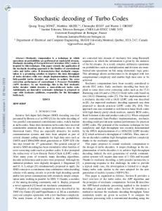
a parity-check code, a single parity-check equation provides for the detection, but not correction, of a single bit inversion in a received codeword. To permit correction of errors induced by channel noise, additional parity checks can be added at the expense of a decrease in the rate of transmission. Low-density parity-check codes are a special case of such codes. Here “low-density” refers to the sparsity of the parity-check matrix characterizing the code. Each parity-check equation checks few message bits, and each message bit is involved in only a few parity-check equations. A delicate balance exists in the construction of appropriate parity-check matrices, since excessive sparsity leads to uselessly weak codes. First presented by Gallager in his 1962 thesis [2], [3], low-density parity-check codes are capable of performance extraordinarily close to the Shannon limit when appropriately decoded. Codes that approach the Shannon limit to within 0.04 of a decibel have been constructed. Fig. 1 shows a comparison of the performance of LDPC codes with the performance of some well known error correction codes. The key to extracting maximal benefit from LDPC codes is soft decision decoding, which starts with a more subtle model for channel-induced errors than simple bit inversions. Rather than requiring that the receiver initially make hard decisions at the channel output, and so insisting that each received bit be assessed as either 0 or 1, whatever is the more likely, soft decision decoders use knowledge of the channel noise statistics to feed probabilistic (or “soft”) information on received bits into the decoder. The final ingredient in implementing soft decision decoders with acceptable decoder complexity are iterative schemes which handle the soft information in an efficient manner. Soft iterative decoders for LDPC codes make essential use of graphs to represent codes, passing probabilistic messages along the edges of the graph. The use of graphs for 4
iterative decoding can be traced to Gallager, although for over 30 years barely a handful of researchers pursued the consequences of Gallager’s work. This situation changed dramatically with the independent rediscovery of LDPC codes by several researchers in the mid-1990s, and graph-based representations of codes are now an integral feature in the development of both the theoretical understanding and implementation of iterative decoders. In this chapter, we begin by introducing parity-checks and codes defined by their parity-check matrices. To introduce iterative decoding we present in Section 3 a harddecision iterative algorithm which is not very powerful, but suggestive of how graphbased iterative decoding algorithms work. The soft-decision iterative decoding algorithm for LDPC codes known as sum-product decoding is presented in Section 4. Section 5 focuses the relationship between the codes and the decoding algorithm, as expressed in the graphical representation of LDPC codes, and Section 6 considers the design of LDPC codes. The chapter concludes with the connections of this work to other topics and future directions in the area.
2 2.1
Low-density parity-check codes Parity-check codes
The simplest possible error detection scheme is the single parity check, which involves the addition of a single extra bit to a binary message. Whether this parity bit should be a 0 or a 1 depends on whether even or odd parity is being used. In even parity, the additional bit added to each message ensures an even number of 1s in each transmitted codeword. For example, since the 7-bit ASCII code for the letter S is 1010011, a parity 5
bit is added as the eighth bit. If even parity is being used, the value of the parity bit is 0 to form the codeword 10100110. More formally, for the 7-bit ASCII plus even parity code we define a codeword c to have the following structure: c = c 1 c2 c3 c4 c5 c6 c7 c8 , where each ci is either 0 or 1, and every codeword satisfies the constraint c1 ⊕ c2 ⊕ c3 ⊕ c4 ⊕ c5 ⊕ c6 ⊕ c7 ⊕ c8 = 0.
(1)
Here the symbol ⊕ represents modulo-2 addition, which is equal to 1 if the ordinary sum is odd and 0 if the ordinary sum is even. While the inversion of a single bit due to channel noise can easily be detected with a single parity check (as (1) is no longer satisfied by the noise-corrupted codeword) this code is not sufficiently powerful to indicate which bit, or bits, were inverted. Moreover, since any even number of bit inversions produces a word satisfying the constraint (1), any even numbers of errors go undetected by this simple code. One measure of the ability of a code to detect errors is the minimum distance of the code. The Hamming distance between two codewords is defined as the number of bit positions in which they differ. For example the codewords 10100110 and 10000111 differ in positions 3 and 8 so the Hamming distance between them is 2. The minimum distance of a code, dmin , is defined as the smallest Hamming distance between any pair of codewords in the code. For the even parity code dmin = 2, so the corruption of two bits in a codeword can result in another valid codeword and will consequently not be detected. Detecting more than a single bit error calls for increased redundancy in the form 6
of additional parity checks. To illustrate, suppose we define a codeword c to have the following structure: c = c 1 c2 c3 c4 c5 c6 , where each ci is either 0 or 1, and c is constrained by three parity-check equations: c1 ⊕ c 2 ⊕ c 4 = 0 ⇐⇒
c2 ⊕ c 3 ⊕ c 5 = 0 c1 ⊕ c 2 ⊕ c 3 ⊕ c 6 = 0
1 1 0 1 0 0 0 1 1 0 1 0 1 1 1 0 0 1 {z } | H
c1 c2 0 c3 = 0 . c4 0 c5 c6
(2)
In matrix form we have that c = [c1 c2 c3 c4 c5 c6 ] is a codeword if and only if it satisfies the constraint HcT = 0,
(3)
where the parity-check matrix, H, contains the set of parity-check equations which define the code. To generate the codeword for a given message, the code constraints can be rewritten in the form c4 = c 1 ⊕ c 2 c5 = c 2 ⊕ c 3
⇐⇒
�
c1 c2 c3 c4 c5 c6
c6 = c 1 ⊕ c 2 ⊕ c 3
�
=
�
1 0 0 1 0 1 � c1 c2 c3 0 1 0 0 1 1 , 0 0 1 1 1 1 | {z } G
(4)
where bits c1 , c2 , and c3 contain the 3-bit message, and parity-check bits c4 , c5 and c6 are calculated from the message. Thus, for example, the message 110 produces paritycheck bits c4 = 1 ⊕ 1 = 0, c5 = 1 ⊕ 0 = 1 and c6 = 1 ⊕ 1 ⊕ 0 = 0, and hence the 7
codeword 110010. The matrix G is the generator matrix of the code. Substituting each of the 23 = 8 distinct messages c1 c2 c3 = 000, 001, . . . , 111 into equation (4) yields the following set of codewords: 000000 001011 010111 011100
(5)
100101 101110 110010 111001. The reception of a word which is not in this set of codewords can be detected using the parity-check constraint equation (3). Suppose for example that the word r = 101011 is received from the channel. Substitution into equation (3) gives
T Hr =
1 1 0 1 0 0 0 1 1 0 1 0 1 1 1 0 0 1
1 0 1 1 = 0 0 1 1 1
(6)
which is nonzero and so the word 101011 is not a codeword of our code. To go further and correct the error requires that the decoder determine the codeword most likely to have been sent. Since it is reasonable to assume that a small number of errors is more likely to occur than a large number, the required codeword is the one closest in Hamming distance to the received word. By comparison of the received word r = 101011 with each of the codewords in (5), the closest codeword is c = 001011, which is at Hamming distance 1 from r. The minimum distance of this code is 3, so a single bit error always results in a word closer to the codeword which was sent than any other codeword, and hence can always be corrected. In general, for a code with minimum distance dmin , e bit errors can always be corrected by choosing the closest codeword 8
whenever e ≤ b(dmin − 1)/2c,
(7)
where bxc is the largest integer that is at most x. Error correction by direct search is feasible only when the number of distinct codewords is small. For codes with thousands of bits in a codeword, it becomes far too computationally expensive to directly compare the received word with every codeword in the code, and numerous ingenious solutions have been proposed, including choosing codes which are cyclic or, as presented in this chapter, devising iterative methods to decode the received word.
2.2
Low-density codes
LDPC codes are parity-check codes with the requirement that H is low-density, so that the vast majority of entries are zero. A parity-check matrix is regular if each code bit is contained in a fixed number, wc , of parity checks and each parity-check equation contains a fixed number, wr , of code bits. If an LDPC code is described by a regular parity-check matrix it is called a (wc ,wr )-regular LDPC code otherwise it is an irregular LDPC code. Importantly, an error correction code can be described by more than one paritycheck matrix, where H is a valid parity-check matrix for a code provided that (3) holds for all codewords in the code. Two parity-check matrices for the same code need not even have the same number of rows; what is required is that the rank over GF(2) of both be the same, since the number of message bits, k, in a binary code is k = n − rank2 (H).
9
(8)
where rank2 (H) is the number of rows in H which are linearly dependent over GF(2). To illustrate we give a regular parity-check matrix for the code of (2) with wc = 2, wr = 3 and rank2 (H) = 3, which satisfies (3): 1 1 0 0 1 1 H= 1 0 0 0 0 1
1 0 0 0 1 0 . 0 1 1 1 0 1
(9)
A Tanner graph is a graphical representation of H which facilitates iterative decoding of the code. The Tanner graph consists of two sets of vertices: n bit vertices (or bit nodes), and m parity-check vertices (or check nodes), where there is a parity-check vertex for every parity-check equation in H and a bit vertex for every codeword bit. Each parity-check vertex is connected by an edge to the bit vertices corresponding to the code bits included in that parity-check equation. The Tanner graph of the paritycheck matrix (9) is shown in Fig. 2. As the number of edges leaving the bit vertices must equal the number of edges leaving the parity-check vertices it follows that for a regular code, m · wr = n · w c .
(10)
A cycle in a Tanner graph is a sequence of connected vertices which start and end at the same vertex in the graph, and which contain other vertices no more than once. The length of a cycle is the number of edges it contains, and the girth of a graph is the size of its smallest cycle. A cycle of size 6 is shown in bold in Fig. 2. Traditionally, the parity-check matrices of LDPC codes have been defined pseudorandomly subject to the requirement that H be sparse, and code construction of binary LDPC codes involves randomly assigning a small number of the values in an all-zero 10
matrix to be 1. The lack of any obvious algebraic structure in randomly constructed LDPC codes sets them apart from traditional parity-check codes. The properties and performance of LDPC codes are often considered in terms of the ensemble performance of all possible codes with a specified structure (for example a certain node degree distribution), reminiscent of the methods used by Shannon in proving his noisy channel coding theorem. Recent research has considered the design of LDPC codes with specific properties, such as large girth, and we describe in Sections 5 and 6 methods to design LDPC codes. For sum-product decoding however, no additional structure beyond a sparse parity-check matrix is required and in the following two sections we present decoding algorithms requiring only the existence of a sparse H.
3
Iterative decoding
To illustrate the process of iterative decoding a bit-flipping algorithm is presented, based on an initial hard decision (0 or 1) assessment of each received bit. An essential part of iterative decoding is the passing of messages between the nodes of the Tanner graph of the code. For the bit-flipping algorithm the messages are simple: a bit node sends a message to each of the check nodes to which it is connected declaring if it is a 1 or a 0, and each check node sends a message to each of the bit nodes to which it is connected, declaring whether the parity check is satisfied or not. The sum-product algorithm for LDPC codes operates similarly but with more complicated messages. The bit-flipping decoding algorithm is as follows: Step 1. Initialization: Each bit node is assigned the bit value received from the channel, and sends messages to the check nodes to which it is connected indicating this 11
value. Step 2. Parity update: Using the messages from the bit nodes, each check node calculates whether or not its parity-check equation is satisfied. If all parity-check equations are satisfied the algorithm terminates, otherwise each check node sends messages to the bit nodes to which it is connected indicating whether or not the parity-check equation is satisfied. Step 3. Bit update: If the majority of the messages received by each bit node are “not satisfied,” the bit node flips its current value, otherwise the value is retained. If the maximum number of allowed iterations is reached the algorithm terminates and a failure to converge is reported, otherwise each bit node sends new messages to the check nodes to which it is connected, indicating its value and the algorithm returns to Step 2. To illustrate the operation of the bit-flipping decoder, we take the code of (9) and again assume that the codeword c = 001011 is sent, and the word r = 101011 is received from the channel. The steps required to decode this received word are shown in Fig. 3. In Step 1 the bit values are initialized to be 1, 0, 1, 0, 1, and 1, respectively, and messages are sent to the check nodes indicating these values. In Step 2 each parity-check equation is satisfied only if an even number of the bits included in the parity-check equation are 1. For the first and third check nodes this is not the case, and so they send “not satisfied” messages to the bits to which they are connected. In Step 3 the first bit has the majority of its messages indicating “not satisfied” and so flips its value from 1 to 0. Step 2 is repeated and since now all four parity-check equations are satisfied, the algorithm halts and returns c = 001011 as the decoded codeword. The received word has therefore been 12
correctly decoded without requiring an explicit search over all possible codewords. The existence of cycles in the Tanner graph of a code reduces the effectiveness of the iterative decoding process. To illustrate the detrimental effect of a 4-cycle we adjust the code of the previous example to obtain the new code shown in Fig. 4. A valid codeword for this code is 001001 but again we assume that the first bit is corrupted, so that r = 101001 is received from the channel. The steps of the bit-flipping algorithm for this received word are shown in Fig. 4. In Step 1 the initial bit values are 1, 0, 1, 0, 0, and 1, respectively, and messages are sent to the check nodes indicating these values. Step 2 reveals that the first and second parity-check equations are not satisfied. In Step 3 both the first and second bits have the majority of their messages indicating “not satisfied” and so both flip their bit values. When Step 2 is repeated we see that the first and second parity-check equations are again not satisfied. Further iterations at this point simply cause the first two bits to flip their values in such a way that one of them is always incorrect; the algorithm fails to converge. As a result of the 4-cycle each of the first two codeword bits are involved in the same two parity-check equations, and so when neither of the parity-check equations are satisfied, it is not possible to determine which bit is causing the error.
4
Sum-product decoding
The sum-product decoding algorithm, also called belief propagation decoding, was first introduced by Gallager in his 1962 thesis where he applied it to the decoding of pseudorandomly constructed LDPC codes. For block lengths of 107 , highly optimized irregular LDPC codes decoded with the sum-product algorithm are now known to be capable
13
of approaching the Shannon limit to within hundredths of a decibel on the binaryinput additive white Gaussian noise (AWGN) channel. In the early 1960s, however, limited computing resources prevented Gallager from demonstrating the capabilities of iteratively decoded LDPC codes for blocklengths longer than around 500, and for over 30 years his work was ignored by all but a handful of researchers. It was only re-discovered by several researchers in the wake of turbo decoding [4], which has subsequently been recognized as an instance of the sum-product algorithm. The sum-product algorithm can be thought of as being similar to the bit-flipping algorithm described in the previous section, but with the messages representing each decision (check met, or bit value equal to 1) now probabilistic values represented by loglikelihood ratios. Whereas with bit-flipping decoding an initial hard decision is made on the signal from the channel, what is actually received is a string of real values where the sign of the received value represents a binary decision, 0 if positive and 1 if negative, and the magnitude of the received value is a measure of the confidence in that decision. A shortcoming of using only hard decisions when decoding is that the information relating to the confidence of the signal, the soft information, is discarded. Soft decision decoders, such as the sum-product decoder, make use of the soft received information, together with knowledge of the channel properties, to obtain probabilistic expressions for the transmitted signal. For a binary signal, if p is the probability of a 1, then 1 − p is the probability of a 0 which is represented as a log-likelihood ratio (LLR) by LLR(p) = loge
�
1−p p
�
.
(11)
The sign of LLR(p) is the hard decision and the magnitude |LLR(p)| is the reliability
14
of this decision. One benefit of the logarithmic representation of probabilities is that whereas probabilities need to be multiplied, log-likelihood ratios need only be added, reducing implementation complexity. The aim of sum-product decoding is to compute the a posteriori probability (APP) for each codeword bit, Pi = P {ci = 1|N }, which is the probability that the ith codeword bit is a 1 conditional on the event N that all parity-check constraints are satisfied. The intrinsic or a priori probability, Piint , is the original bit probability independent of knowledge of the code constraints, and the extrinsic probability Piext represents what has been learnt from the event N . The sum-product algorithm iteratively computes an approximation of the APP value for each code bit. The approximations are exact if the code is cycle free. Extrinsic information gained from the parity-check constraints in one iteration is used as a priori information for the subsequent iteration. The extrinsic bit information obtained from a parity-check constraint is independent of the a priori value for that bit at the start of the iteration. The extrinsic information provided in subsequent iterations remains independent of the original a priori probability until that information is returned via a cycle. To compute the extrinsic probability of a codeword bit i from the jth parity-check equation we determine the probability that the parity-check equation is satisfied if bit i is assumed to be a 1, which is the probability that an odd number of the other codeword bits are a 1, Pi,j =
1 1 + 2 2
Y
i0 ∈B
j
(1 − 2Piint 0 ).
(12)
,i0 6=i
The notation Bj represents the set of column locations of the bits in the jth parity-check equation of the code considered. Similarly, Ai is the set of row locations of the parity15
check equations which check on the ith bit of the code. To put (12) into log-likelihood notation we note that tanh
�
1 loge 2
�
1+
Q
1−p p
��
= 1 − 2p,
to give ext LLR(Pi,j ) = loge
1−
Q
,i0 6=i
tanh(LLR(Piint 0 )/2)
i0 ∈Bj , i0 6=i
tanh(LLR(Piint 0 )/2)
i0 ∈B
j
!
.
The LLR of the estimated APP of the ith bit at each iteration is then simply LLR(Pi ) = LLR(Piint ) +
X
ext LLR(Pi,j ).
j∈Ai
The sum-product algorithm is as follows: Step 1. Initialization: The initial message sent from bit node i to the check node j is the LLR of the (soft) received signal yi given knowledge of the channel properties. For an AWGN channel with signal-to-noise ratio Eb /N0 this is: Li,j = Ri = 4yi
Eb . N0
(13)
Step 2. Check-to-bit: The extrinsic message from check node j to bit node i is the probability that parity-check j is satisfied if bit i is assumed to be a 1 expressed as an LLR: Ei,j = loge
1+ 1−
Q
Q
i0 ∈Bj ,i0 6=i
tanh(Li0 ,j /2)
i0 ∈Bj , i0 6=i
tanh(Li0 ,j /2)
!
.
(14)
Step 3. Codeword test: The combined LLR is the sum of the extrinsic LLRs and the original LLR calculated in Step 1: Li =
X
Ei,j + Ri .
j∈Ai
For each bit a hard decision is made: 1, Li ≤ 0 zi = 0, Li > 0. 16
(15)
If z = [z1 , . . . , zn ] is a valid codeword (Hz T = 0), or if the maximum number of allowed iterations have been completed, the algorithm terminates. Step 4. Bit-to-check : The message sent by each bit node to the check nodes to which it is connected is similar to (15), except that bit i sends to check node j a LLR calculated without using the information from check node j: Li,j =
X
j 0 ∈A
i,
Ei,j 0 + Ri .
(16)
j 0 6=j
Return to Step 2. The application of equations (14) and (16) to the code in (9) is demonstrated in Fig. 5. The extrinsic information passed from a check node to a bit node is independent of the probability value for that bit. The extrinsic information from the check nodes is then used as a priori information for the bit nodes in the subsequent iteration. To illustrate the power of sum-product decoding we revisit the example of Fig. 3 where the codeword sent is 0 0 1 0 1 1. Suppose that the channel is AWGN with Eb /N0 = 1.25 and the received signal is y = −0.1
0.5
− 0.8
1.0
− 0.7
0.5.
There are now two bits in error if the hard decision of the signal is considered: bits 1 and 6. Fig. 6 illustrates the operation of the sum-product decoding algorithm, as described in equations (13)–(16), to decode this received signal which terminates in three iterations. The existence of an exact termination rule for the sum-product algorithm has two important benefits; the first is that a failure to converge is always detected, and the second is that additional iterations once a solution has been found are avoided. There are variations to the sum-product algorithm presented here. The min-sum algorithm, for example, simplifies the calculation of (14) by recognizing that the term corresponding to the smallest Li0 ,j dominates the product term and so the product 17
can be approximated by a minimum; the resulting algorithm thus requires calculation of only minimums and additions. An alternative approach, designed to bridge the gap between the error performance of sum-product decoding and that of maximum-likelihood (ML) decoding, finishes each iteration of sum-product decoding with ordered statistic decoding, with the algorithm terminating when a specified number of iterations have returned the same codeword [5].
5
Codes, graphs and cycles
The relationship between LDPC codes and their decoding is closely associated with the graph-based representations of the codes. The most obvious example of this is the link between the existence of cycles in the Tanner graph of the code to both the analysis and performance of sum-product decoding of the code. In his work, Gallager used a graphical representation of the bit and parity-check sets of regular LDPC codes, to describe the application of iterative APP decoding. The systematic study of codes on graphs however is largely due to Tanner who, in 1981, extended the single parity-check constraints of Gallager’s LDPC codes to arbitrary linear code constraints, foresaw the advantages for very large-scale integration (VLSI) implementations of iterative decoders, and formalized the use of bipartite graphs for describing families of codes [6]. In doing so, Tanner also founded the topic of algebraic methods for constructing graphs suitable for sum-product decoding. By proving the convergence of the sum-product algorithm for codes whose graphs are free of cycles, Tanner was also the first to formally recognize the importance of cyclefree graphs in the context of iterative decoding. The effect of cycles on the practical
18
performance of LDPC codes was demonstrated by simulation experiments when LDPC codes were rediscovered by MacKay and Neal [7] (among others) in the mid-1990s, and the beneficial effects of using graphs free of short cycles were shown [8]. Given the detrimental effects of cycles on the convergence of iterative decoders, it is natural to seek strong codes whose Tanner graphs are free of cycles. An important negative result in this direction was established by Etzion et al. [9], who showed that for linear codes of rate k/n ≥ 0.5 which can be represented by a Tanner graph without cycles, the minimum distance is at most 2. As the existence of cycles in a graph makes analysis of the decoding algorithm difficult, most analyses consider the asymptotic performance of iterative decoding on graphs with asymptotically unbounded girth. This analysis provides thresholds to the performance of LDPC codes with sum-product decoding. As we will see in the following section, this process can be used to select LDPC code properties which improve the threshold values, a process which works well even though the resulting codes contain cycles. To date very little analysis has been presented regarding the convergence of iterative decoding methods on graphs with cycles, and the majority of the work in this area can be found in [10]. Gallager suggested that the dependencies introduced by cycles have a relatively minor effect and tend to cancel each other out somewhat. This “seems to work” philosophy has underlined the performance of sum-product decoding on graphs with cycles for much of the (short) history of the topic. It is only recently that exact analysis on the expected performance of codes with cycles has emerged. The recent paper of Di et al. [11] uses finite length analysis to give the exact average bit and block error probabilities for any regular ensemble of LDPC codes over the binary erasure 19
channel when decoded iteratively, however there is as yet no such analysis for irregular codes or more general channel models. Besides cycles, Sipser and Spielman [12] showed that the expansion of the graph is a significant factor in the application of iterative decoding. Using only a simple hard decision decoding algorithm they proved that a fixed fraction of errors in an LDPC code can be corrected in linear time provided that the Tanner graph of the code is a good enough expander. That is, any subset S of bit vertices of size m or less is connected to at least �|S| constraint vertices, for some defined m and �.
6
Designing LDPC codes
For the most part, LDPC codes are designed by first choosing the required blocklength and node degree distributions, then pseudo-randomly constructing a parity-check matrix, or graph, with these properties. A generator matrix for the code can then be found using Gaussian elimination [8]. Gallager, for example, considered the ensemble of all (wr , wc )-regular matrices with rows divided into wc submatrices, the first containing wr copies of the identity matrix and with subsequent submatrices being random column permutations of the first. Using ensembles of matrices defined in this way Gallager was able to find the maximum crossover probability of the binary symmetric channel (BSC) for which LDPC codes could be used to transmit information reliably using a simple hard decision decoding algorithm. Luby et al. extended the class of LDPC ensembles to those with irregular node degrees and showed that irregular codes are capable of outperforming regular codes [13]. In extending Gallagers analysis to irregular ensembles, Luby et al. introduced
20
tools based on linear programming for designing irregular code ensembles for which the maximum allowed crossover probability of the binary symmetric channel is optimized [14]. Resulting from this work are the so-called “tornado codes,” a family of codes that approach the capacity of the erasure channel and can be encoded and decoded in linear time. Richardson and Urbanke extended the work of Luby et al. to any binary input memoryless channel and to soft decision message passing decoding [15]. They determined the capacity of message passing decoders applied to LDPC code ensembles by a method called density evolution. For sum-product decoding density evolution makes it possible to determine the corresponding capacity to any degree of accuracy and hence determine the ensemble with node degree distribution which gives the best capacity. Once a code ensemble has been chosen a code from that ensemble is realized pseudo-randomly. By carefully choosing a code from an optimized ensemble Chung et al. have demonstrated the best performance to date of LDPC codes in terms of approaching the Shannon limit [16]. A recent development in the design of LDPC codes is the introduction of algebraic LDPC codes, the most promising of which are the finite geometry codes proposed by Lucas et al. [17] which are cyclic and described by sparse 4-cycle free graphs. An important outcome of this work with finite geometry codes was the demonstration that highly redundant parity-check matrices can lead to very good iterative decoding performances without the need for very long blocklengths. While the probability of a random graph having a highly redundant parity-check matrix is vanishingly small, the field of combinatorial designs offers a rich source of algebraic constructions for matrices which are both sparse and redundant. In particular, there has been much recent interest in 21
balanced incomplete block designs (BIBDs) to produce sparse matrices for LDPC codes which are 4-cycle free. For codes with greater girth, generalized quadrangle designs give the maximum possible girth for a graph with given diameter [18]. Both generalized quadrangles and BIBDs are subsets of the more general class of combinatorial structures called partial geometries, a possible source of further good algebraic LDPC codes [19]. In comparison with more traditional forms of error correcting codes, the minimum distance of LDPC codes plays a substantially reduced role. There are two reasons for this: firstly, the lack of any obvious algebraic structure in pseudo-randomly constructed LDPC codes makes the calculation of minimum distance infeasible for long codes, and most analyses focus on the average distance function for an ensemble of LDPC codes. Secondly, the absence of conspicuous flattening of the bit-error rate (BER) curve at moderate to high signal-to-noise ratios (the so-called “error floor”) strongly suggests that minimum distance properties are simply not as important for LDPC codes as for traditional codes. Indeed, it has recently been established that to achieve capacity on the binary erasure channel when using irregular LDPC codes, the codes cannot have large minimum distances [20].
7
Connections and future directions
Following the rediscovery of Gallager’s iterative LDPC decoding algorithm in the mid1990s, the notion of an iterative algorithm operating on a graph has been generalized and is now capable of unifying a wide range of apparently different algorithms from the domains of digital communications, signal processing, and even artificial intelligence. An important generalization of Tanner graphs was presented by Wiberg in his 1996 PhD
22
thesis [21]. Wiberg introduced state variables into the graphical framework, thereby establishing a connection between codes on graphs and the trellis complexity of codes, and was the first to observe that on cycle-free graphs, the sum-product (respectively, min-sum) algorithm performs APP (respectively, ML) decoding. In an even more general setting, the role of the Tanner graph is taken by a factor graph [22]. Central to the unification of message-passing algorithms via factor graphs is the recognition that many computationally efficient signal processing algorithms exploit the way in which a global cost function acting on many variables can be factorized into the product of simpler local functions, each of which operates on a subset of the variables. In this setting a (bipartite) factor graph encodes the factorization of the global cost function, with each local function node connected by edges only to those variable nodes associated with its arguments. The sum-product algorithm operating on a factor graph uses message-passing to solve the marginalize product-of-functions (MPF) problem which lies at the heart of many signal processing problems. In addition to the iterative decoding of LDPC codes, specific instances of the sum-product algorithm operating on suitably defined factor graphs include the forward/backward algorithm (also known as the BCJR (Bahl–Cocke– Jelinek–Raviv) algorithm [23] or APP decoding algorithm), the Viterbi algorithm, the Kalman filter, Pearl’s belief propagation algorithm for Bayesian networks, and the iterative decoding of “turbo codes,” or parallel concatenated convolutional codes. For high-performance applications, LDPC codes are naturally seen as competitors to turbo codes. LDPC codes are capable of outperforming turbo codes for block lengths greater than around 105 , and the error floors of LDPC codes at BERs below about 10−5 are typically much less pronounced than those of turbo codes. Moreover, the inherent 23
parallelism of the sum-product decoding algorithm is more readily exploited with LDPC codes than their turbo counterparts, where block interleavers pose formidable challenges to achieving high throughput [24]. Despite these impressive advantages, LDPC codes lag behind turbo codes in real-world applications. The exceptional simulation performance of the original turbo codes [4, 25] generated intense interest in these codes, and variants of them were subsequently incorporated into proposals for third-generation (3G) wireless systems such as the Third Generation Partnership Project (3GPP), a global consortium of standards-setting organizations [26]. Whatever performance advantages of very long LDPC codes over turbo codes there may be, the invention of turbo codes some three years prior to the (re-)discovery of LDPC codes has given them a distinct advantage in wireless communications, where blocklengths of at most several thousand are typical, and where compliance with global standards is paramount. One serious shortcoming of LDPC codes is their potentially high encoding complexity, which is in general quadratic in the blocklength, and compares poorly with the linear time encoding of turbo codes. Finding computationally efficient encoders is therefore critical for LDPC codes to be considered as serious contenders for replacing turbo codes in future generations of forward error correction devices. Several approaches have been suggested, including the manipulation of the parity-check matrix to establish that while the complexity is, strictly speaking, quadratic, the actual number of encoding operations grows essentially linearly with blocklength. For some irregular LDPC codes whose degree distributions have been optimized to allow transmission near to capacity, the encoding complexity can be shown to be truly linear in blocklength [27]. A very different approach to the encoding complexity problem is to employ cyclic, or quasi-cyclic, codes as LDPC codes, as encoding can be achieved in linear time using simple feedback shift 24
registers [28]. While addressing encoding complexity is driven by applications, two issues seem likely to dominate future theoretical investigations of LDPC codes. The first of these is to characterize the performance of LDPC codes with ML decoding and so to assess how much loss in performance is due to the structure of the codes, and how much is due to the sub-optimum iterative decoding algorithm. The second, and related, issue is to rigorously deal with the decoding of codes on graphs with cycles. Most analyses to date have assumed that the graphs are effectively cycle-free. What is not yet fully understood is just why the sum-product decoder performs as well as it does with LDPC codes having cycles.
References [1] C. E. Shannon, “A mathematical theory of communication,” Bell Syst. Tech. J., vol. 27, pp. 379–423, 623–656, July–Oct. 1948. [2] R. G. Gallager, “Low-density parity-check codes,” IRE Trans. Inform. Theory, vol. IT-8, no. 1, pp. 21–28, January 1962. [3] R. G. Gallager, Low-Density Parity-Check Codes, MIT Press, Cambridge, MA, 1963. [4] C. Berrou, A. Glavieux, and P. Thitimajshima,
“Near Shannon limit error-
correcting coding and decoding: Turbo-codes,” in Proc. IEEE Int. Conf. on Communications (ICC’93), Geneva, Switzerland, May 1993, pp. 1064–1070.
25
[5] M. P. C. Fossorier, “Iterative reliability-based decoding of low-density parity check codes,” IEEE J. Selected Areas Commun., vol. 19, no. 5, pp. 908–917, May 2001. [6] R. M. Tanner, “A recursive approach to low complexity codes,” IEEE Trans. Inform. Theory, vol. IT-27, no. 5, pp. 533–547, September 1981. [7] D. J. C. MacKay and R. M. Neal, “Near Shannon limit performance of low density parity check codes,” Electron. Lett., vol. 32, no. 18, pp. 1645–1646, March 1996, Reprinted Electron. Lett, vol. 33, no. 6, pp. 457–458, March 1997. [8] D. J. C. MacKay, “Good error-correcting codes based on very sparse matrices,” IEEE Trans. Inform. Theory, vol. 45, no. 2, pp. 399–431, March 1999. [9] T. Etzion, A. Trachtenberg, and A. Vardy, “Which codes have cycle-free Tanner graphs?,” IEEE Trans. Inform. Theory, vol. 45, no. 6, pp. 2173–2181, September 1999. [10] “Special issue on Codes on Graphs and Iterative Algorithms,” IEEE Trans. Inform. Theory, vol. 47, no. 2, February 2001. [11] C. Di, D. Proietti, I. E. Telatar, T. J. Richardson, and R. L. Urbanke, “Finitelength analysis of low-density parity-check codes on the binary erasure channel,” IEEE Trans. Inform. Theory, vol. 48, no. 6, pp. 1570–1579, June 2002. [12] M. Sipser and D. A. Spielman, “Expander codes,” IEEE Trans. Inform. Theory, vol. 42, no. 6, pp. 1710–1722, November 1996. [13] M. G. Luby, M. Mitzenmacher, M. A. Shokrollahi, and D. A. Spielman, “Efficient erasure correcting codes,” IEEE Trans. Inform. Theory, vol. 47, no. 2, pp. 569–584, February 2001. 26
[14] M. G. Luby, M. Mitzenmacher, M. A. Shokrollahi, and D. A. Spielman, “Improved low-density parity-check codes using irregular graphs,” IEEE Trans. Inform. Theory, vol. 47, no. 2, pp. 585–598, February 2001. [15] T. J. Richardson and R. L. Urbanke, “The capacity of low-density parity-check codes under message-passing decoding,” IEEE Trans. Inform. Theory, vol. 47, no. 2, pp. 599–618, February 2001. [16] S.-Y. Chung, G. D. Forney, Jr., T. J. Richardson, and R. Urbanke, “On the design of low-density parity-check codes within 0.0045 dB of the Shannon limit,” IEEE Commun. Letters, vol. 5, no. 2, pp. 58–60, February 2001. [17] R. Lucas, M. P. C. Fossorier, Y. Kou, and S. Lin, “Iterative decoding of onestep majority logic decodable codes based on belief propagation,” IEEE Trans. Commun., vol. 48, no. 6, pp. 931–937, June 2000. [18] P. O. Vontobel and R. M. Tanner, “Construction of codes based on finite generalized quadrangles for iterative decoding,” in Proc. IEEE Int. Symp. Inform. Theory., Washington, DC, June 24–29 2001, p. 223. [19] S. J. Johnson and S. R. Weller, “Codes for iterative decoding from partial geometries,” in Proc. IEEE Int. Symp. Inform. Theory., Lausanne, Switzerland, June 30–July 5 2002, p. 310. [20] C. Di, T. J. Richardson, and R. L. Urbanke, “Weight distributions: How deviant can you be?,” in Proc. IEEE Int. Symp. Inform. Theory., Washington, DC, June 24–29 2001, p. 50.
27
[21] N. Wiberg, Codes and Decoding on General Graphs, Ph.D. thesis, Link¨oping University, S-581 83 Link¨oping, Sweden, Department of Electrical Engineering, 1996. [22] F. R. Kschischang, B. J. Frey, and H.-A. Loeliger, “Factor graphs and the sumproduct algorithm,” IEEE Trans. Inform. Theory, vol. 47, no. 2, pp. 498–519, February 2001. [23] L. R. Bahl, J. Cocke, F. Jelinek, and J. Raviv, “Optimal decoding of linear codes for minimizing symbol error rate,” IEEE Trans. Inform. Theory, vol. IT-20, no. 2, pp. 284–287, March 1974. [24] A. J. Blanksby and C. J. Howland, “A 690-mW 1-Gb/s 1024-b, rate-1/2 lowdensity parity-check code decoder,” IEEE J. Solid-State Circuits, vol. 37, no. 3, pp. 404–412, March 2002. [25] C. Berrou and A. Glavieux, “Near optimum error correcting coding and decoding: Turbo codes,” IEEE Trans. Commun., vol. 44, no. 10, pp. 1261–1271, October 1996. [26] “3rd Generation Partnership Project (3GPP); Technical specification group radio access network; Multiplexing and channel coding (FDD), 3GPP TS 25.212 V4.0.0 (2000-12),” [Online]. Available: http://www.3gpp.org. [27] T. J. Richardson and R. L. Urbanke, “Efficient encoding of low-density parity-check codes,” IEEE Trans. Inform. Theory, vol. 47, no. 2, pp. 638–656, February 2001.
28
[28] Y. Kou, S. Lin, and M. P. C. Fossorier, “Low-density parity-check codes based on finite geometries: A rediscovery and new results,” IEEE Trans. Inform. Theory, vol. 47, no. 7, pp. 2711–2736, November 2001.
29
−1
10
Shannon Limit Irregular LDPC Turbo Regular LDPC Soft Viterbi
−2
10
−3
Bit error rate
10
−4
10
−5
10
−6
10
0
0.5
1
1.5
2
2.5 E /N (dB) b
3
3.5
4
4.5
5
0
Figure 1: Bit error rate performance of rate-1/2 error correction codes on an additive white Gaussian noise channel. From right to left, soft Viterbi decoding of a constraint length 7 convolutional code; sum-product decoding of a regular Gallager code with blocklength 65389 [8]; a turbo code with 2 + 32 states, 16384 bit interleaver, and 18 iterations ; sum-product decoding of a blocklength 107 optimized irregular code [16]; and the Shannon limit at rate 1/2
check vertices
bit vertices
Figure 2: Tanner graph representation of the parity-check matrix in (9). A 6-cycle is shown in bold.
30
Parity update
Initialization
1
0
1
0
1
Bit update
0
1
1
0
1
0
1
1
Parity update
0
1
0
1
0
1
0
1
0
1
1
Figure 3: Bit-flipping decoding of the received word r = 101011. Each sub-figure indicates the decision made at each step of the decoding algorithm based on the messages from the previous step. A cross (×) represents that the parity check is not satisfied while a tick (X) indicates that it is satisfied. For the messages, a dashed arrow corresponds to the messages “bit = 0” or “check not satisfied,” while a solid arrow corresponds to “bit = 1” or “check satisfied”.
Parity update
Initialization
1
0
1
0
0
0
1
0
0
1
Parity update
Bit update
0
1
1
1
1
0
0
0
1
1
1
0
0
1
Figure 4: Bit-flipping decoding of the received word r = 101001. A 4-cycle is shown in bold in the first sub-figure.
31
rag replacements
E1,1
L1,1
L4,1
E1,3
L2,1 R1 E1,1 = log
�
1+tanh(L2,1 /2)·tanh(L4,1 /2) 1−tanh(L2,1 /2)·tanh(L4,1 /2)
�
L1,1 = E1,3 + R1
Figure 5: An example of the messages for sum-product decoding. Calculation of the extrinsic message sent to bit 1 depends on messages from bits 2 and 4 but not from bit 1. Similarly, the message sent to check 1 is independent of the message just received from it.
32
Iteration 1 R =
�
−0.5000
2.5000 −4.0000
[ 1 0 1 0 1 0 ]
as a hard decision
�
2.4217 −0.4930 . −0.4217 . . · 3.0265 −2.1892 . −2.3001 · −2.1892 . . . −0.4217 0.4696 · . 2.4217 −2.3001 . −3.6869
=
L
=
z
= [ 1 0 1 0 1 1 ]
Hz T
= [ 1 0 1 0 ]
�
−0.2676
5.0334 −3.7676
T
⇒
=
E
=
L
=
z
= [ 0 0 1 1 1 1 ]
Hz T
= [ 1 0 0 1 ]
Iteration 2
2.5000
E
L
5.0000 −3.5000
−2.6892 · 1.9217 ·
�
2.2783 −6.2217 −0.7173
�
Continue
5.5265 · 2.0070 −1.5783 . · . −6.1892
2.6999 · · . −3.9217 · · −5.8001 −1.1869 4.5783 . 2.9696
2.6426 −2.0060 . −2.6326 . . · 1.4907 −1.8721 . −1.1041 . 1.1779 · · . −0.8388 −1.9016 · . 2.7877 −2.9305 · −4.3963 3.3206
1.9848 −3.0845 −0.5630 −5.4429 −3.7979
T
⇒
�
Continue
=
0.6779 · 2.1426 ·
3.9907 · 0.4940 −1.2123 · · · −5.8721
E
=
1.9352 · 1.8332 ·
L
=
3.2684
4.1912 −3.9896
z
�
0.5180 . 0.6515 . · 1.1733 −0.4808 . −0.2637 · · · · −1.3362 −2.0620 · 0.4912 −0.5948 · −2.3381
= [ 0 0 1 0 1 1 ]
Hz T
= [ 0 0 0 0 ]
L
Iteration 3
T
⇒
2.0695 . · . −4.3388 · · −4.6041 −1.8963 2.3674 · 0.5984
5.0567 −5.0999 −1.9001
�
Terminate
Figure 6: Operation of sum-product decoding with the code from (9) when the codeword [001011] is sent through an AWGN channel with Eb /N0 = 1.25 and the vector [-0.1 0.5 -0.8 1.0 -0.7 0.5] is received. The sum-product decoder converges to the correct codeword after three iterations. 33