REPLACE THIS LINE WITH YOUR PAPER IDENTIFICATION NUMBER (DOUBLE-CLICK HERE ... decoding of a polar code with length of N, totally 2(N-1) clock.
> REPLACE THIS LINE WITH YOUR PAPER IDENTIFICATION NUMBER (DOUBLE-CLICK HERE TO EDIT)
REPLACE THIS LINE WITH YOUR PAPER IDENTIFICATION NUMBER (DOUBLE-CLICK HERE TO EDIT) < (1st decoder) and its sub-blocks, such as the merged PE and the ICG module is discussed in block Section IV. In Section V, based on the one given in Section IV three modified decoders are presented, which employ unfolding (2nd decoder), folding (3rd decoder), and parallel processing techniques (4th decoder), respectively. The 2nd decoder architecture is compatible with M consecutive inputs processing. The 3rd one time-multiplexes all decoding operations on a single PE stage. Using the same number of PEs as the 3rd one, the 4th decoder manages to implement 2-parallel processing at the price of an additional clock cycle. It is obvious to see that compared with the 1st design, each variant improves the hardware efficiency while keeps the same low-latency advantage. The corresponding performance estimation and comparison with state-of-the-art designs are presented in Section VI. Section VII concludes the paper.
label attached to each PE indicates the index of clock cycle when the corresponding PE is activated. stage 3
3
stage 2
2
stage 1
1
L(81) ( y 18 )
L(11) ( y 1 ) 10
9
8
6
5
1
13
12
uˆˆ1 + u2
8
4
2
uˆˆ5 + u6
1
L(85 ) ( y 18 , uˆ14 ) L(83 ) ( y 18 , uˆ12 ) L(87 ) ( y 18 , uˆ16 )
uˆˆˆˆ 1 + u2 + u3 + u 4
uˆˆ3 + u4
L(82 ) ( y 18 , uˆ1 )
In this section, we provide the preliminaries of the SC decoding algorithm. Moreover, some variants and simplified modifications of the SC algorithm are explained as well. A. SC Decoding Algorithm Consider an arbitrary polar code with parameter (N, K, , u c ) [1]. We denote the input vector as u1N , which consists of a random part u and a frozen part u c . The corresponding output vector through channel W N is y1N with conditional probability WN ( y1N | u1N ) . Define the likelihood ratio (LR) as, W (i ) ( y N , uˆ i −1 | 0) (1) L(Ni ) ( y1N , uˆ1i −1 ) N(i ) 1N 1i −1 . WN ( y1 , uˆ1 | 1) The a posteriori decision scheme is given as follows,
A Posteriori Decision Scheme with Frozen Bits c then uˆi =ui; 1: if i ∈ 2: else 3: 4:
if L ( y , uˆˆ1i −1 ) ≥ 1 then ui =0; else uˆi =1; (i ) N
N 1
5: endif 6: endif It is noted that LRs with even and odd indices can be generated by applying the recursive formulas given by Eq. (2) and (3), respectively: L(2N i ) ( y1N , uˆ12i −1 ) (2) 2i − 2 2 i − 2 1− 2 uˆ2 i −1 ⋅ L(Ni ) 2 ( y NN 2 +1 , u1,2ie− 2 ), =[L(Ni ) 2 ( y1N 2 , uˆˆˆ 1, o ⊕ u1, e )]
L(11) ( y 4 ) L(11) ( y 5 )
11
uˆ1
9
8
7
uˆ 5
5
1
L(86 ) ( y 18 , uˆ15 )
L(11) ( y 2 ) L(11) ( y 3 )
uˆˆ2 + u4
L(84 ) ( y 18 , uˆ13 )
ˆ 14 u3
ˆ 13 u2
uˆ 7
uˆ 6 : Type I PE
L(11) ( y 6 ) L(11) ( y 7 )
8
L(88 ) ( y 18 , uˆ17 )
II. REVIEW OF SC ALGORITHM AND ITS VARIANTS
2
uˆ 4
L(11) ( y 8 )
: Type II PE
Figure 1: SC decoding process of polar codes with length N = 8.
B. SC Decoding Algorithm in Logarithm Domain For any general decoding algorithm, its variant defined in logarithm domain always has advantages in terms of hardware implementation, computational complexity, and numerical stability over the one in real domain. Therefore, similar to the approach addressed in [5], the SC algorithm dealing with logarithm-likelihood ratio (LLR) was mentioned by [3]. Eq. (4) and (5) can then be rewritten as follows: (2Ni ) ( y1N , uˆ12i −1 ) (4) 2i − 2 2i − 2 (i ) 2i − 2 N =(-1)uˆ2 i−1 (Ni ) 2 ( y1N 2 , uˆˆˆ 1, o ⊕ u1, e ) + N 2 ( y N 2 +1 , u1, e ),
(2Ni -1) ( y1N , uˆ12i −1 ) =2artanh{tanh[(Ni ) 2 ( y1N 2 , uˆˆ1,2io− 2 ⊕ u1,2ie− 2 )] ⋅ tanh[(Ni ) 2 ( y NN 2 +1 , uˆ1,2ie− 2 )]}. Here the LLRs are defined as: (Ni ) ( y1N , uˆˆ1i −1 ) ln L(Ni ) ( y1N , u1i −1 ).
(5)
(6)
C. Min-Sum SC Decoding Algorithm In order to implement the hyperbolic tangent function and its inverse function in Eq. (5), large amount of look-up table (LUT) is required. Note that in logarithm domain, for variable x ≫ 1, the following approximation holds: (7) ln[cosh( x)] x − ln 2.
Consequently, Eq. (5) can be reduced to the min-sum update rule, which is LUT free: (2Ni -1) ( y1N , uˆ12i − 2 ) 1 N 2i − 2 2i − 2 (i ) 2i − 2 ⋅ (Ni ) 2 ( y1N 2 , uˆˆˆ 1, o ⊕ u1, e ) + N 2 ( y N 2 +1 , u1, e ) − L(2N i -1) ( y1N , uˆ12i − 2 ) 2 2i − 2 2i − 2 (i ) N 2i − 2 1 (i ) N 2i − 2 2i − 2 (i ) 2i − 2 L(Ni ) 2 ( y1N 2 , uˆˆˆ (3) 1, o ⊕ u1, e ) LN 2 ( y N 2 +1 , u1, e ) + 1 (8) ⋅ N 2 ( y1N 2 , uˆˆˆ 1, o ⊕ u1, e ) − N 2 ( y N 2 +1 , u1, e ) = (i ) . 2 N 2 2i − 2 2i − 2 (i ) N 2i − 2 N 2 N (i ) 2i − 2 2i − 2 (i ) 2i − 2 LN 2 ( y1 , uˆˆˆ u L y u ⊕ )+ ( , ) 1, o 1, e N 2 N 2 +1 1, e = sgn[ , uˆˆˆ N 2 ( y1 1, o ⊕ u1, e )]sgn[ N 2 ( y N 2 +1 , u1, e )] ⋅ N 2i − 2 2i − 2 (i ) 2i − 2 Obviously, the calculation of L(Ni ) ( y1N , uˆ1i −1 ) depends on the min[ (Ni ) 2 ( y1N 2 , uˆˆˆ 1, o ⊕ u1, e ) , N 2 ( y N 2 +1 , u1, e ) ]. estimation of the previous bit, from which the SC decoding Simulation results have demonstrated that the min-sum SC algorithm is named. For the ease of clear explanation, the decoding algorithm only suffers from little performance decoding procedure of a polar code with N = 8 is illustrated in degradation than the optimal one while achieves a good Fig. 1, where Type I and Type II PEs are in charge of hardware efficiency [3]. This property makes min-sum SC computations given in Eq. (2) and (3), respectively. And the
> REPLACE THIS LINE WITH YOUR PAPER IDENTIFICATION NUMBER (DOUBLE-CLICK HERE TO EDIT) < decoding algorithm very attractive for VLSI implementation. Therefore, in the following sections we will discuss the polar decoder design based on this sub-optimal algorithm. However, among all those decoding algorithms pre-stated, probabilities are updated according to the same data flow illustrated in Fig. 1, which is straightforward but not efficient enough. In the next section, we present our high-performance scheme for polar decoder design. In the proposed scheme, compared to the schemes presented above, the number of clock cycles required for obtaining the estimated information bits has been reduced by 50%. Moreover, this latency-reduced scheme is suitable for any code length N, and can be generated in a nice recursive manner. III. PROPOSED LATENCY-REDUCED UPDATING SCHEME FOR POLAR DECODER DESIGN In what follows, we present a latency-reduced updating scheme for polar decoders based on a novel look-ahead scheduling method. The proposed techniques need fewer number of clock cycles to perform the same operation as the conventional SC decoding algorithm, leading to lower decoding latency. For the straightforward SC decoding implementation of N-bit polar codes, totally 2(N-1) clock cycles are required. Careful investigation has shown that the corresponding time chart can be constructed in recursive way, which is described by the following pseudo-codes. In an effort for conciseness, in the rest of this paper, the notation TC = {[ , TC], s} is used for the left insertion of an array into the previously arranged time chart TC at Stage s. Similarly, TC = [TC, TC] simply means duplication of previous time chart.
active. For ease of clear explanation, the polar decoding process shown in Fig. 1 is employed for detailed illustration. Since block length N = 8, according to Eq. (9) totally 14 clock cycles are required to finish the whole decoding process. The corresponding decoding time chart is given in Fig. 2 (a). However, this conventional decoding approach is not suitable for practical applications for the following two reasons. First, in order to achieve required decoding performance, the code length N is usually set to be as large as 210-220. An immediate consequence is the latency of 2(N-1) clock cycles is too large. Second, according to Fig. 2 (a), it is apparent that during the whole decoding process the highest hardware utilization in a specific clock cycle is only 50% (Clock cycle 1). As the stage index increases, the hardware efficiency will go down as low as 12.5%. For general case with code length of N, the minimum hardware efficiency for active stage is 1/N (Clock cycle log 2 N). Since only polar codes with code length greater or equal than 210 can achieve a good performance that approaching the channel capacity, the straightforward implementation in Fig. 1 becomes impractical for real-life applications because the lowest hardware usage can be around 2-10. Even for the pipelined tree architecture proposed by [3] in Fig. 3, the highest utilization is only 50% as well, which means half PEs are in idle state during each clock cycle. Stage 3
Stage 2
Stage 1
L(11) ( y 1 ) L(12 i −1) ( y 18 , uˆ12 i −2 )
L(11) ( y 2 ) L(11) ( y 3 )
Recursive Construction of Conventional Time Chart 1: initializtion TC=;
L(11) ( y 4 )
3: = j log 2 N − i + 1;
L(11) ( y 6 )
L(11) ( y 5 )
2: = for i log 2 N , i − −,1 do
4: TC = {[ j of Type I, TC], i}; 5: TC = [TC, TC]; 6: change the leftmost j of Type I with j of Type II; 7: endfor 8: output TC. Here, i and j are indices of iterative execution. “j of Type I” is the short for j copy (or copies) of Type I PE(s). Basically, Stage i will be activated 2i times during the whole decoding process. Therefore, the total number of clock cycles required can be calculated as follows: log 2 N −1 (2log2 N − 1) (9) 2 ∑ 2i = 2⋅ 2( N − 1), = 2 −1 i =0 which matches the general conclusion given before. According to Fig. 1, it can be observed that each PE is activated only once during the entire decoding process. In one specific clock cycle only single type of PE is active. The output LLRs will be generated the same clock cycle in which the log 2 N-th stage is
3
L(12 i ) ( y 18 , uˆ12 i −1 )
L(11) ( y 7 ) L(11) ( y 8 )
: Type I PE
: Type II PE
: Pipeline
Figure 3: Pipelined decoder architectures of polar codes with length N = 8.
This dilemma is introduced by the bottleneck of sequential decoding property of SC algorithm. In order to address this issue properly, the computation loop can be re-scheduled with look-ahead techniques. However, in order to achieve the goal of low latency and high performance, the new decoding schedule needs to be carefully chosen. It is noted that if both the two LLR inputs for Eq. (5) are available, there are only two possible outputs. Therefore, for any Type I PE, given two deterministic LLR inputs, the look-ahead scheme only needs to pre-compute two output candidates. The correct output can be selected by a multiplexer thereafter. For the instance shown in Fig. 1, all possible outputs of Type I PEs labeled by 8 in Stage 1 can be pre-calculated in Clock cycle 1. In other words, for Stage 1 the required computation in Clock cycle 8 can be incorporated into
> REPLACE THIS LINE WITH YOUR PAPER IDENTIFICATION NUMBER (DOUBLE-CLICK HERE TO EDIT)
REPLACE THIS LINE WITH YOUR PAPER IDENTIFICATION NUMBER (DOUBLE-CLICK HERE TO EDIT) < Yq-1
X2
Y2
X1
Y1
X0
Y0
… Bq Cq
B3 1-bit full Bq-1 1-bit full B2 1-bit full B1 1-bit full … 1-bit adder full 1-bit adder full 1-bit adder full 1-bit half adder … adder Cq-1 adder adder C1 adder C3 C2
1
… Dq-1 Sq-1
D2 S2
D1 S1
D0 S0
Figure 4: q-bit adder-subtractor architecture.
As shown in Fig.4, in order to avoid large processing latency, parallel implementation is employed here. However, simple duplication results in penalty of doubling both area and power. For a q-bit adder-subtractor, totally 2q-1 1-bit full adder and one 1-bit half adder are required. In order to implement Type-I PE more effectively, the novel architecture of adder-subtractor is proposed in this section. Rather than implementing Type-I PE with two’s complement approach, the original carry-borrow idea is employed here. Suppose X and Y are the two operands, and Z in is the carried-in or borrowed-from bit. For the full adder the two outputs of summation and carry-out are represented by S and C out , respectively. In similar way, the difference and borrow-out produced by the full subtructor are denoted with D and B out . Therefore, the truth table for the full adder and subtractor is given below. TABLE I TRUTH TABLE OF BOTH FULL ADDER AND SUBTRACTOR Outputs Inputs Adder Subtructor X Y Z in S C out D B out 0 0 0 0 0 0 0 0 0 1 1 0 1 1 0 1 0 1 0 1 1 0 1 1 0 1 0 1 1 0 0 1 0 1 0 1 0 1 0 1 0 0 1 1 0 0 1 0 0 1 1 1 1 1 1 1
hardware complexities are converted in the form of equivalent XOR gate number. According to Fig. 5, the complexities of 1-bit full and half adder-subtractor equal to 4 XOR gates and 1 XOR gate, respectively. Compared with the straightforward ones, the total savings of the proposed approaches are 43% and 50%, respectively. Composed of q-1 1-bit full adder-subtractor and a 1-bit half adder-subtractor, the general q-bit adder-subtractor architecture with the given design method requires only less than 57% hardware compared with the conventional one while achieves exactly the same performances.
Cout = X ⋅ Y + ( X ⊕ Y ) ⋅ Z in ; D = X ⊕ Y ⊕ Z in ;
Bout = X ⋅ Y + X ⊕ Y ⋅ Z in .
(11)
X
Bout
Y S
Cin Cout
(a) 1-bit full adder-subtractor. X
Bout
S D
Y
Cout
(b) 1-bit half adder-subtractor. Figure 5: Proposed 1-bit adder-subtractor architectures.
Without being misunderstood, it is agreed that hereinafter the newly proposed Type I PE illustrated in Fig. 6 is still referred to as “Type I PE”. The Type I PE with the conventional architectures will not be employed or discussed any more. Xq-1 Bq
From Table I one can draw the Karnaugh map for all outputs based on which the logic equations are derived as follows: (10) S = X ⊕ Y ⊕ Z in ;
Bin
D
Cq
X1
Yq-1
Bq-1 … 1-bit full adderC q-1 subtractor …
Sq-1
Dq-1
B2 C2
…
Y1
1-bit full addersubtractor
S1
X0
Y0
B1
1-bit half adderC1 subtractor
S0
D1
D0
Xq-1
5
X
Y
Type I PE
S
D
Figure 6: Proposed Type I PE architectures.
(12) (13)
It is obvious that outputs S and D are actually the same. And easy to notice that X ⋅ Y is an intermediate term of X ⊕ Y . Similarly, ( X ⊕ Y ) ⋅ Z in can be treated as a byproduct of term X ⊕ Y ⊕ Z in as well. Since both outputs C out and B out can be calculated by recursively employing the AND or AND-NOT operation twice, they can be obtained simultaneously with other two outputs. The resulted gate-sharing techniques can not only implement parallel processing but also reduce the hardware consumption. The proposed gate-level structures of 1-bit full and half adder-subtractor are depicted in Fig. 5 (a) and (b) respectively, where the carry-in bit C in and borrow-out bit B in are supposed to be different rather than in the unique form of Z in . For the sake of easy estimation and comparison, all the
B. Design of Type II PE output q
TtoS
input 1 q
TtoS
input 2 q
sgn sgn
StoT
mag
q
q CMP
mag
Type II PE q N 2 i −2 (i ) input 1: N 2 ( y N 2+1, uˆ 1,e ); input 2 : (Ni ) 2 ( y 1N 2 , uˆˆ12,oi −2 ⊕ u12,ei −2 ); output: ( 2 i -1) ( y N , uˆ 2 i −2 ). N 1 1
Figure 7: Proposed architectures of Type II PE.
Instead of implementing tanh and artanh functions, Type II PE which employs the min-sum algorithm is shown in Fig.7. TtoS block will perform the conversion from two’s complement
> REPLACE THIS LINE WITH YOUR PAPER IDENTIFICATION NUMBER (DOUBLE-CLICK HERE TO EDIT) < representation to sign-magnitude representation. StoT block will perform the reverse conversion. The TtoS block is illustrated in Fig. 8. In order to avoid the overflow situation, a sign extension operation is required as well. Iq-1
I2
I1
I0
1 0
1 0
1 0
… 1 0 …
1-bit half adder
… Cq-1
C3
1-bit half adder
C2
1-bit half adder
C1
1-bit half adder
C0
Type I PE to process the computation. Moreover, for efficient execution of each Type I PE, the value of uˆ2i −1 needs to be provided on the fly. However, even for the 8-bit decoder illustrated in Fig. 1, the complicated interleaving of odd and even indices makes the straightforward calculation of uˆ2i −1 inconvenient. In order to solve this inherent problem, the input generating circuit (IGC) for Type I PEs is proposed in this section. Careful investigation has shown that it is possible to generate the required uˆ2i −1 using the real FFT-like signal flow. For an instance, all the extra input values uˆ2i −1 for 8-bit polar code decoder can be easily generated according to the following in-place procedure. Stage 1
Oq
…
Oq-1
O2
O1
O0
uˆ1
Figure 8: Proposed structure of TtoS block. uˆ 2
The StoT block is similar to the TtoS block. The only difference is that a sign compression operation is needed to make the output data in the form of the q-bit quantization. C. Sub-structure Sharing of Type I and Type II PEs Since the comparator in Type II PE is actually a q-bit subtractor, which is also employed by Type I PE, it is possible to incorporate both Type I and Type II PEs together using the sub-structure sharing scheme. The detailed structure is illustrated as follows:
uˆˆ1 + u2
output 1 q
q
StoT
0 1
output 2 q output 3 q
StoT StoT
Bn
q
0 1
q
mag
sgn
1 0
q q
mag
TtoS TtoS
input 1 q input 2 q
S
D
Type I PE
Stage 2
uˆˆ3 + u4
uˆˆ3 + u4
uˆ 3 uˆ 4 uˆ 5 uˆ 6 uˆ 7 uˆ 8
uˆˆˆˆ 1 + u2 + u3 + u 4
uˆˆ2 + u4
uˆ 2
uˆ 4
uˆ 4 uˆˆˆˆ 5 + u6 + u7 + u8
uˆˆ5 + u6
uˆˆ6 + u8
uˆ 6 uˆˆ7 + u8
uˆˆ7 + u8
uˆ 8
: XOR operation sgn
Merged PE
6
uˆ 8
: PASS operation
Figure 11: Flow graph of IGC for 8-point polar decoder.
Here, the pass operation process element only lets the lower input get through. According to Fig. 11, the flow graph can be further simplified with the properties explained as follows: 1. The first simplification is to consider that all outputs which are not necessary. be removed. Similar concept can be applied to the general case of N inputs. For any Stage i, its lower region which contains 2i process elements (PEs), can be removed. For example, the lower 2 PEs of Stage 1 and the lower 4 PEs of Stage 2 are removed from the flow graph in Fig. 11. Therefore, only (N/2)(log 2 N-1) outputs need to be computed. 2. The second simplification refers to the fact that the PASS operation element can be replaced by the wire connection while the flow graph stays functionally the same. According to Fig. 11, element only allow the lower input through to the next stage. Thus, if the upper token is not treated as an input to element any more, one simple wire which connects the lower token and the output can be employed instead. Meanwhile, complexity of the flow graph can be halved with respect to the former one.
( 2 i -1) 2 i −2 N (Ni ) 2 ( y NN 2+1, uˆ 12,ei −2 ); are associated with inputs uˆ NN −1 input 1: output 2 : N ( y 1 , uˆˆ1 ), u2 i −1 = 0; ( 2 i -1) 2 i −2 2 i −2 2 i −2 N ⊕ , = input 2 : (Ni ) 2 ( y 1N 2 , uˆˆˆˆ output : 1 ); ( , ) . u y u u 1,o 1,e 3 1 1 2 i −1 N Consequently, the shaded region can output 1: ( 2 i -1) ( y N , uˆ 2 i −2 ); 1 1 N
Figure 9: Proposed structure of the Merged PE.
In the Merged PE, the comparison operation is carried out by the Type I PE illustrated Fig. 6. Two more StoT blocks as well as additional control logic are required here. According to Fig. 9, for q-bit quantization scheme totally 2q-3 XOR gates can be saved by the proposed sub-structure sharing approach. As mentioned previously, usually code length N over 210 is a must for polar codes to achieve required decoding performances in practical applications. For conventional pipelined tree polar decoder architectures, N-1 Merged PEs can be employed instead of N-1 Type I PEs and Type II PEs, respectively. As a consequence, the resulted hardware saving could be around 210∙(2q-3) XOR gates. D. Input Generating Circuit for Type I PEs
As indicated in Eq. (5), except for (Ni ) 2 ( y1N 2 , uˆˆ1,2io− 2 ⊕ u1,2ie− 2 ) and (Ni ) 2 ( y NN 2 +1 , uˆ1,2ie− 2 ) , another input uˆ2i −1 is also required by
The resulted simplified data flow graph is given in Fig. 12. Both properties have been fully utilized. It is easy to see that totally log 2 N-1 stages are required and the number of XOR
> REPLACE THIS LINE WITH YOUR PAPER IDENTIFICATION NUMBER (DOUBLE-CLICK HERE TO EDIT) < operations is calculated below: [ N (log 2 N − 1) − 2(1 − N 2) (1 − 2)] 2
(14)
uˆˆˆˆ 1 + u2 + u3 + u 4
uˆˆ2 + u4 uˆˆ3 + u4
In general, for N-bit length decoder, since the data structures of IGC are defined recursively for powers of 2, the unfolded pipelined architecture can be constructed with the recurrence relationship. The recursion for the general case is shown in Fig. 15, where module U n can be constructed based on module U n-1 and N/4 extra XOR-pass elements. Here, we have n = log 2 N-1. And the control bit c n can be obtained by down sampling c 1 by a factor of n.
D … D D
0
uˆ 2 i −1
where B N is the bit-reversal permutation matrix and F matrix is defined as: 1 0 (16) F . 1 1 The pipelined architecture of the simplified flow graph illustrated in Fig. 12 can be implemented with the following feed-forward architecture, where totally two XOR-pass elements are required.
Stage n 2n-1-1
cn 1
…
2n-1-1 D … D D
0 1
…
…
Un-1
2n-1-1 D … D D
0
uˆ 2 i
1
N/2 outputs
In addition, it is worthwhile to note that with the help of generator matrix G N [1], the same simplified flow graph can be obtained as well. We define ⨂ to be the matrix Kronecker product and n equals log 2 N. Then the generator matrix G N is given by the following equation: ⊗n (15) = GN B= F ⊗ n BN , NF
…
Figure 12: Simplified flow graph of the proposed IGC.
…
uˆ 4
uˆ 6
uˆ 6
U2
Figure 14: Unfolded version of pipelined architecture in Fig. 13.
uˆˆ5 + u6
uˆ 5
U1
…
uˆ 4
uˆ 4
1
…
uˆˆ3 + u4
uˆ 3
D
0
uˆ 2 i
…
uˆ 2
uˆ 2
1
…
uˆˆ1 + u2
D
0
uˆ 2 i −1
…
uˆ1
Stage 2
c1
4 outputs
Stage 1
Stage 2
Stage 1
= N (log 2 N − 2) 2 + 1.
7
Un
Figure 15: Recursive construction of U n based on U n-1 . Stage 2
Therefore, the total number of XOR-pass elements can be calculated as: n−2
2 ∑=
(17)
i =0
Figure 13: Pipelined feed-forward architecture for 8-bit IGC.
Stage n
1
… … 0 1
Un-1
…
RAMn …
uˆ2i
0 1
addr.
…
0
uˆ21i −
…
cn
N/2 outputs
Easily to observe that the proposed pipelined architecture is only suitable for serial inputs. However, as indicated by the time chart illustrated in Fig. 2 (b), every two decoded bits are output in the same clock cycle. In order to work compatibly with this schedule, the architecture needs to be modified to make itself a 2-level parallel processing structure, which is shown in Fig. 14. The control bit c 1 is changed with the clock flipping manner and its initial value is set to be 0. By unfolding the i-th stage with the unfolding factor of 2i-1, the updated input generating circuit is able to create 2i outputs at the same time, which the original circuit does in 2i-1 consecutive clock cycles. For example, the unfolded version of the circuit shown in Fig. 13 is given as follows, where U i denotes the unfolded pipelined architecture which is consists of i stage(s):
N 2 − 1.
i
…
D D
…
D D
…
uˆ 2 i
D
2 outputs
uˆ 2 i −1
…
Stage 1
Un
Figure 16: Recursive construction of U n based on U n-1 using RAMs.
Also it is easy to see that the same amount of demultiplexers is required. Finally, as what we expect, the obtained pipelined
> REPLACE THIS LINE WITH YOUR PAPER IDENTIFICATION NUMBER (DOUBLE-CLICK HERE TO EDIT) < structure works best with the proposed time chart, which enables all intermediate results to be generated in place without any extra clock cycles. However, it can be noticed that for Stage i, the number of corresponding registers increases with the complexity of 2i, which is obviously impractical for polar codes of length over 210. One possible approach is to employ memory banks instead of flip-flops, which is shown in Fig. 16. For RAM i , totally 2i-1 memory elements are required. And the data lifetime is 2i-2-1 clock cycles, according to which the memory enable signals can be therefore determined. E. Pipelined Architecture of the Look-Ahead Decoder Taking the advantage of the pre-stated modules, the overall pipelined architecture of the proposed look-ahead decoder can be designed accordingly. Without of loss of generality, here we employ an 8-bit polar decoder as an example. Fig.17 shows the proposed pipelined architecture for a 8-bit look-ahead polar decoder, which is composed of the main computation structure and the IGC part. It is a feed-forward pipelined structure that tries to maximize the use of the hardware and minimize the latency of decoding. Stage 3
Stage 2
: Pipeline
O2
0
uˆˆ1 + u2 or uˆˆ5 + u6
O1 I1
0
O2
1
O3 I2
O I L(11) ( y 2 ) uˆˆˆˆ + u + u + u 1 2 3 4 3
O3 I2
1
L(12 i −1) ( y 18 , uˆ12 i −2 )
1
2
O1 I1
O3 I2
1
uˆˆ3 + u4
O1 I1
uˆˆ2 + u4
O3 I2
1
signs
O3 I2
1
O2
uˆˆ2 or u6
c1 RAM2
O1 I1
0
O2
1
O3 I2
0 1
L(11) ( y 6 ) L(11) ( y 7 )
Stage 3 and 3'
L(11) ( y 8 )
uˆ 4
Stage 2
Stage 1
0
L(12 i −1) ( y 18 , uˆ12 i −2 ) 4 outputs
1
L(11) ( y 5 )
: Pipeline
0
L(11) ( y 4 )
O2
0
0
L(11) ( y 3 )
O2
0
O1 I1
L(12 i ) ( y 18 , uˆ12 i −1 )
TABLE II REFINED DECODING SCHEDULES OF 8-POLAR DECODER Clock cycle Stage 1 2 3 4 5 6 7 8 Look-ahead decoding schedule –– –– –– –– –– –– 1 C1 C2 –– –– –– –– –– –– 2 C1 C1 –– –– –– –– 3 C1 C1 C1 C1 Look-ahead decoding schedule with refined pipelining –– –– –– –– 1 C1 C2 C3 C4 –– –– 2 C1 C2 C3 C1 C2 C3 –– –– 3 C1 C2 C3 C1 C2 C3 –– –– –– 3’ C1 C2 C3 C1 C2
L(11) ( y 1 )
O2
0 O1 I1
decoder architectures, the hardware utilization of each active stage is 100%, other stages still remain idle at the same time. Moreover, for the proposed 8-bit polar decoder, totally 7 clock cycles are required before the next codeword can be processed. Generally, for an N-bit polar decoder each codeword needs N-1 clock cycles to be properly decoded with the given approach, during which no new codeword could be input to the decoder. Therefore, even only half latency is needed by the proposed scheme, the hardware efficiency remains low for decoders with large N. Meanwhile, in synthesizing DSP architectures it is also important to maximize the silicon efficiency of the integrated circuits. One possible approach is to further refine the pipelined architecture which enables new input every clock cycle [6]. According to the decoding time chart depicted in Fig. 2 (b), the new decoding schedule which triples the decoding throughput is given in Table II. In order to process three codewords simultaneously, Stage 3 has been duplicated (Stage 3’) to avoid data contradiction. It is obvious to see that the hardware efficiency for stage i (i > 1) is 85.7%. And that of Stage 1 is 42.9%. Compared with similar approach in [3], the proposed one achieves the same utilization rate at each stage but is better arranged, which can be observed from Table II of [3] easily.
Stage 1 O1 I1
8
L(12 i ) ( y 18 , uˆ12 i −1 )
O1 I1
0
O2
0
1
O3 I2
1
D D D D
O1 I1
D D D
O3 I2
1
0
uˆˆ1 + u2 or uˆˆ5 + u6
U1 U2
1
In general, for the N-bit polar decoder, totally N-1 incorporated PEs, 2N-3 2-to-1 multiplexers, N/2-1 XOR-PASS elements, N/2-2 1-to-2 demultiplexers, 3(N-1) delay elements, and N/2-2 bits of RAM are required.
L
(2 i ) 1
L
2 i −2 1
8 1
( y , uˆ 8 1
2 i −1 1
( y , uˆ
)
0
)
O1 I1
0
O2
0
1
O3 I2
1
O1 I1
D D D
O3 I2
1
0 1
{3, 6}
uˆ 4
6l+3, 6 {4, 1}
{2, 5}
c1 RAM2 RAM2 0c1 c RAM2 1 0 1
1 2 3
{3, 6}
0
O1 I1
D D D
O3 I2
L(11) ( y 4 )
D D D D
O1 I1
L(11) ( y 5 )
D D D
O3 I2
L(11) ( y 6 )
D D D D
O1 I1
L(11) ( y 7 )
D D D
O3 I2
{4}
{5}
U1 U1 U1
L(11) ( y 2 ) L(11) ( y 3 )
O2
O2
O2
{6}
1
1 0
{4, 1}
{3, 6}
D D D D
1 0
{5, 2}
{5, 2}
O3 I2
uˆˆ2 + u4
O2
{1, 4}
signs
In this section, we propose the systematic design methods for three different modified look-ahead polar decoders based on the one illustrated in Fig. 17. DSP-VLSI design techniques are well employed to improve the hardware efficiency while keep the reduced decoding latency unchanged. 1) Refined Pipelined Architecture of the Look-Ahead Decoder It is easy to notice that although for the proposed pipelined
D D D D
uˆˆ2 or u6
V. MODIFIED ARCHITECTURES FOR PROPOSED DECODER
D D D
O2
uˆˆ3 + u4
Figure 17: Pipelined decoder of look-ahead polar codes with N = 8. ( 2 i −1) 1
O1 I1
uˆˆˆˆ 1 + u2 + u3 + u 4
O2
L(11) ( y 1 )
D D D D
1 0
U1 2 U2 U2
Figure 18: Refined pipelined decoder of polar codes with N = 8.
L(11) ( y 8 )
> REPLACE THIS LINE WITH YOUR PAPER IDENTIFICATION NUMBER (DOUBLE-CLICK HERE TO EDIT) < Without loss of generality, here the authors use the refined architecture of 8-bit polar decoder as an example, which is illustrated in Fig. 18. Other decoders with different code length can be derived accordingly. It is worth noting that Stage 3 and 3’, which are activated in serial, are generated by unfolding transformation with factor of 2. Keeping in mind that the concurrent 3 inputs are independent, totally 3 copies of IGC are required as a result. According to the recursive construction algorithm of look-ahead time chart given in Section III, it is obvious that for N-bit polar decoder the maximum value of concurrent inputs is N-1. However, in order to guarantee the non-blocking decoding process, more duplicated stages are required by higher concurrent number M. The detailed relationship between concurrent number and hardware consumption can be stated in the following properties. Property 1 For N-bit look-ahead polar decoder, the highest concurrent number M is N-1. Proof According to recursive algorithm, the decoding time chart will take totally log 2 N −1 2log2 N − 1 i (18) 2= = N −1 ∑ 2 −1 i =0 clock cycles. During the decoding process for a single codeword, Stage 1 is only activated in one clock cycle. Therefore, in the rest N-2 clock cycles, Stage 1 is available for other possible input codewords.∎ Property 2 For a given N-bit polar decoder architecture, the 2i-1 concurrent version can be derived by duplicating 2i-1-1 stages, which have the most significant indices, of the 2i-1-1 concurrent version.
9
in the method given in Property 2.∎ For example, the 3-concurrent version of 8-bit look-ahead polar decoder in Table II is implemented by adding a duplicated Stage 3 to the 1-concurrent version. Moreover, its 7-concurrent version, which can achieve 100% efficiency, can be constructed based on the 3-concurrent version accordingly as follows in Table III. Since 7 = 23 -1 (20) , 3-1 3= 2 -1 the 7-concurrent version can be derived based on the 3-concurrent one by duplicate Stage 2, 3, and 3’, which have the most significant indices. It can be seen that the proposed 7-concurrent decoder can handle inputs perfectly and achieve 100% utilization rate during Decoding iteration i (i > 1). Property 3 For any M which satisfies 2i-1-1 < M ≤2i-1, the M-concurrent polar decoder requires the same hardware consumption. And 100% hardware efficiency can be achieved if and only if when M = 2i-1. Proof According to the proof of Property 2, the proof is immediate and its details are omitted here.∎ Property 4 For any M which satisfies 2i-1-1 < M ≤2i-1, the totally number of PEs employed by the M-concurrent polar decoder is N+2i-1∙(i-2). Proof According to Property 1, the number of PEs can be calculated as follows: log 2 N −1
∑
2i + 2i −1 ⋅ (i − 1)
j = i −1
Proof It can be noticed that 2i = − 1 2(2i −1 − 1) + 1,
= ( N − 2i −1 ) + 2i −1 ⋅ (i − 1) (19)
which is in the same manner that the look-ahead decoding chart is constructed. In order to make 100% hardware utilization of the whole decoder (or certain specific stages), for each decoding stage the number of PEs should stay the same. Since the decoding chart is constructed in the time domain, we only need to apply the same approach in the “stage domain”, which results
= N +2
i −1
(21)
⋅ (i − 2).
For example, the 1-, 3-, and 7-concurrent versions of 8-bit look-ahead polar decoder are calculated to have 7, 8, and 12 PEs respectively, which can be easily verified according to Table II and III.
TABLE III 3- AND 7-CONCURRENT DECODING SCHEDULES OF 8-BIT POLAR DECODER Stage
1
2
3
1 2 3 3’
C1 –– –– ––
C2 C1 –– ––
C3 C2 C1 ––
1 2 3 3’ 2’ 3’’ 3’’’
C1 –– –– –– –– –– ––
C2 C1 –– –– –– –– ––
C3 C2 C1 –– –– –– ––
Clock cycle 4 5 6 7 8 9 3-concurrent look-ahead decoding schedule –– –– –– –– C4 C5 –– C3 C1 C2 C3 C4 –– C2 C3 C1 C2 C3 C1 C2 C3 C1 C2 C3 7-concurrent look-ahead decoding schedule C4 C5 C6 C7 ⋯ C3 C4 C5 C6 C7 ⋯ C2 C3 C4 C5 C6 C7 C1 C2 C3 C4 C5 C6 –– C1 C2 C3 C4 C5 –– –– C1 C2 C3 C4 –– –– –– C1 C2 C3
10
11
12
13
14
C6 C5 C4 ––
–– C6 C5 C4
–– C4 C6 C5
–– C5 C4 C6
–– C6 C5 C4
⋯ C7 C6 C5 C4
⋯ C7 C6 C5
⋯ C7 C6
⋯ C7
⋯
> REPLACE THIS LINE WITH YOUR PAPER IDENTIFICATION NUMBER (DOUBLE-CLICK HERE TO EDIT)
REPLACE THIS LINE WITH YOUR PAPER IDENTIFICATION NUMBER (DOUBLE-CLICK HERE TO EDIT)
REPLACE THIS LINE WITH YOUR PAPER IDENTIFICATION NUMBER (DOUBLE-CLICK HERE TO EDIT) < meet demands of different application situations. VII. CONCLUSION Based on the recursive construction method of decoding time chart, a novel look-ahead SC decoding schedule for polar codes is proposed in this paper, which can halve the decoding latency required by conventional approaches. For efficient hardware implementation issue, a Merged PE is presented by using sub structure sharing technique. Its control signal uˆ2i −1 can be generated with a real FFT-like diagram. This unique feature is directly applied to develop an efficient input generating circuit (IGC), which works best with the latency-reduced polar decoder architecture. The methodology for designing four different look-ahead polar decoder architectures is presented along with gate-level details. Comparison results have shown that aside from the IGC module, the proposed designs show comparable hardware efficiency while have much shorter decoding latency than their conventional counterparts. REFERENCES [1]
[2]
[3]
[4]
[5]
[6] [7]
E. Arikan, “Channel polarization: a method for constructing capacity-achieving codes for symmetric binary-input memoryless channels,” IEEE Transactions on Information Theory, vol. 55, no. 7, pp. 3051-3073, July 2009. E. Arkan, “A performance comparison of polar codes and Reed-Muller codes,” IEEE Communications Letters, vol. 12, no. 6, pp. 447-449, June 2008. C. Leroux, I. Tal, A. Vardy, and W. J. Gross, “Hardware architectures for successive cancellation decoding of polar codes,” IEEE International Conference on Acoustics, Speech and Signal Processing (ICASSP), pp. 1665-1668, May 2011. M. Garrido, K. K. Parhi, and J. Grajal, “A pipelined FFT architecture for real-valued signals,” IEEE Transactions on Circuits and Systems I: Regular Papers, vol. 56, no. 12, pp. 2634-2643, Dec. 2009. F. R. Kschischang, B. J. Frey, H.-A. Loeliger, “Factor graphs and the sum-product algorithm,” IEEE Transactions on Information Theory, vol. 47, no. 2, pp. 498-519, Feb 2001. K. K. Parhi, VLSI Digital Signal Processing Systems: Design and Implementation, New York, NY: John Wiley & Sons Inc., 1999. Xinmiao Zhang and Fang Cai, “Efficient Partial-Parallel Decoder Architecture for Quasi-Cyclic Nonbinary LDPC Codes,” IEEE Transactions on Circuits and Systems I: Regular Papers, vol. 58, no. 2, pp. 402-414, Feb. 2011.
12