Low-Rank Tensor Modeling for Hyperspectral Unmixing Accounting

1

Low-Rank Tensor Modeling for Hyperspectral Unmixing Accounting for Spectral Variability

arXiv:1811.02413v1 [cs.CV] 2 Nov 2018

Tales Imbiriba, Member, IEEE, Ricardo Augusto Borsoi, Student Member, IEEE, José Carlos Moreira Bermudez, Senior Member, IEEE

Abstract—Traditional hyperspectral unmixing methods neglect the underlying variability of spectral signatures often obeserved in typical hyperspectral images, propagating these missmodeling errors throughout the whole unmixing process. Attempts to model material spectra as members of sets or as random variables tend to lead to severely ill-posed unmixing problems. To overcome this drawback, endmember variability has been handled through generalizations of the mixing model, combined with spatial regularization over the abundance and endmember estimations. Recently, tensor-based strategies considered lowrank decompositions of hyperspectral images as an alternative to impose low-dimensional structures on the solutions of standard and multitemporal unmixing problems. These strategies, however, present two main drawbacks: 1) they confine the solutions to lowrank tensors, which often cannot represent the complexity of realworld scenarios; and 2) they lack guarantees that endmembers and abundances will be correctly factorized in their respective tensors. In this work, we propose a more flexible approach, called ULTRA-V, that imposes low-rank structures through regularizations whose strictness is controlled by scalar parameters. Simulations attest the superior accuracy of the method when compared with state-of-the-art unmixing algorithms that account for spectral variability. Index Terms—Hyperspectral data, endmember variability, tensor decomposition, low-rank, ULTRA, ULTRA-V.

I. I NTRODUCTION Hyperspectral imaging has attracted formidable interest from the scientific community in the past two decades, and hyperspectral images (HI) have been explored in a vast, and increasing, number of applications in different fields [1]. The limited spatial resolution of hyperspectral devices often mixes the spectral contributions of different pure materials, termed endmembers, in the scene [2]. This phenomenon is more explicit in remote sense applications, due to the distance between airborne and spaceborne sensors and the target scene. The mixing process must be well understood for the vital information relating the pure materials and their distribution in the scene to be accurately unveiled. Hyperspectral unmixing (HU) aims at solving this problem by decomposing the hyperspectral image into a collection of endmembers and their fractional abundances [3]. Different mixing models have been employed to explain the interaction between light and the endmembers [1]-[4]. This work has been supported by the National Council for Scientific and Technological Development (CNPq). R.A. Borsoi, T. Imbiriba and J.C.M. Bermudez are with the Department of Electrical Engineering, Federal University of Santa Catarina, Florianópolis, SC, Brazil. e-mail: [email protected]; [email protected]; [email protected].

The simplest and most widely used model is the Linear Mixing Model (LMM) [2], which assumes that the observed reflectance vector (i.e. a pixel) can be modeled as a convex combination of the spectral signatures of each endmember present in the scene. Convexity imposes positivity and sumto-one constraints on the linear combination coefficients. Hence, they represent the fractional abundances with which the endmembers contribute to the scene. Though the simplicity of the LMM leads to fast and reliable unmixing strategies in some situations, it turns out to be simplistic to explain the mixing process in many practical applications. Hence, several approaches have been proposed in the literature to account for nonlinear mixing effects [4]–[6] and endmember variability [7]–[9] often present in practical scenes. A myriad of factors can induce endmember variability, including environmental, illumination, atmospheric and temporal changes [7]. If not properly considered, such variability can result in significant estimation errors being propagated throughout the unmixing process [10]. Most of the methods proposed so far to deal with spectral variability can be classified in three major groups: endmembers as sets, endmembers as statistical distributions and, more recently, methods that incorporate the variability in the mixing model, often using physically motivated concepts [8]. The method proposed in this work belongs to the third group. Recently, [10], [11] and [12] introduced variations of the LMM to cope with the spectral variability. Unmixing using these models lead to ill-posed problems that were solved by using a combination of different regularizations terms and variable splitting optimization strategies. The model Perturbed LMM (PLMM) in [10] augmented the endmember matrix with an additive perturbation matrix that needs to be estimated jointly with the abundances. Although the additive perturbation can model arbitrary endmember variations, it is not physically motivated, and the excessive amount of degrees of freedom makes the problem even harder to solve. The Extended LMM (ELMM) proposed in [11] introduces one new multiplicative term for each endmember, and can efficiently model changes in the observed reflectance due to illumination effects [11]. This model has a clear physical motivation, but its modeling capability is limited. The Generalized Linear Mixing Model (GLMM) proposed in [12] generalizes the ELMM to account for variability in all regions of the measured spectrum. The GLMM is physically motivated and capable of modeling arbitrary variability, resulting in improved accuracy at the expense of a small increase in the computational complexity, when compared to the ELMM.

2

The above mentioned methods resort to different strategies to regularize the ill-posed optimization problem leading to the estimation of abundances and endmembers. The regularization is achieved by introducing into the unmixing problem additional information based on common knowledge about the low-dimensionality of structures embedded in hyperspectral images. Possible ways to recover lower-dimensional structures from noisy and corrupted data include the imposition of low-rank matrix constraints on the estimation process [13], or the lowrank decomposition of the observed data [14], [15]. The facts that HIs are naturally represented and treated as tensors, and that low-rank decompositions of higher-order (ą2) tensors tend to capture homogeneities within the tensor structure make such strategies even more attractive for HU. Low-rank tensor models have been successfully employed in various tasks involving HIs, such as recovery of missing pixels [16], anomaly detection [17], classification [18], compression [19], dimensionality reduction [20] and analysis of multi-angle images [21]. More recently, [22] and [21] considered low-rank tensor decompositions applied to standard and multitemporal HU, respectively. In [22] the HI is treated as three-dimensional tensor, and spatial regularity is enforced through a nonnegative tensor factorization (NTF) strategy that imposes a low-rank tensor structure. In [21], nonnegative canonical polyadic decomposition were used to unmix multitemporal HIs represented as three-dimensional tensors built by stacking multiple temporal matricized HIs. Though a low-rank tensor representation may naturally describe the regularity of HIs and abundance maps, the forceful introduction of stringent rank constraints may prevent an adequate representation of fast varying structures that are important for accurate unmixing. Another limitation of the approaches proposed in [22] and [21] is the lack of guarantee that endmembers and abundances will be correctly factorized into their respective tensors. In [23], we proposed a new low-rank HU method called Unmixing with Low-rank Tensor Regularization Algorithm (ULTRA), which accounts for highly correlated endmembers. The HU problem was formulated using tensors and a low-rank abundance tensor regularization term was introduced. Differently, from the strict tensor decomposition considered in [21], [22], ULTRA allowed important flexibility to the rank of the estimated abundance tensor to adequately represent fine scale structure and details that lie beyond a low-rank structure, but without compromising the regularity of the solution. In this work we extend the strategy proposed in [23] to account for endmember variability. A second low-rank regularization is imposed on the four-dimensional endmember tensor, which contains one endmember matrix for each pixel. The strategy results in an iterative algorithm, named Unmixing with Low-rank Tensor Regularization Algorithm accounting for endmember Variability (ULTRA-V). At each iteration, ULTRA-V updates the estimations of the abundance and endmember tensors as well as their low-rank approximations. One important challenge of using rank-based approximations is that determination of the rank of tensors is a difficult task. An important contribution of this work is the proposition of a

strategy to determine the smallest rank representation that contains most of the variation of multilinear singular values [24]. Simulation results using synthetic and real data illustrate the performance improvement obtained using ULTRA-V when compared to competing methods, as well as its competitive computational complexity for relatively small images. The paper is organized as follows. Section II briefly reviews important background on linear mixing models and definitions and notation used for tensors. Section III presents the proposed solution and the strategy to estimate tensor ranks. Section IV presents the simulation results and comparisons. Finally, Section V presents the conclusions.

II. BACKGROUND AND NOTATION A. Extended Linear Mixing Models The Linear Mixing Model (LMM) [2] assumes that a given pixel r n “ rrn,1 , . . . , rn,L sJ , with L bands, is represented as r n “ M αn ` en subject to 1J αn “ 1 and αn ľ 0

(1)

where M “ rm1 , . . . , mR s is an L ˆ R matrix whose columns are the R endmembers mi “ rmi,1 , . . . , mi,L sJ , αn “ rαn,1 , . . . , αn,R sJ is the abundance vector, e „ N p0, σn2 I L q is an additive white Gaussian noise (WGN), I L is the L ˆ L identity matrix, and ľ is the entrywise ě operator. The LMM assumes that the pure material endmembers are fixed for all pixels r n , n “ 1, . . . , N , in the HI. This assumption can jeopardize the accuracy of estimated abundances in many circumstances due to the spectral variability existing in a typical scene. Different extensions of the LMM have been recently proposed to mitigate this limitation. These models employ a different endmember matrix for each pixel, and are particular cases of the model r n “ M n αn ` e n

(2)

where M n is the endmember matrix for the n-th pixel. Different parametric models propose different forms for M n to account for spectral variability. These include additive perturbations over a mean matrix in the PLMM [10], multiplicative factors applied individually to each endmember in the ELMM [11] or to each band in the GLMM [12]. Moreover, spatial regularization of the multiplicative scaling factors in the ELMM and GLMM help to further mitigate the ill-posedness of the problem. These models, however, barely exploit the high dimensional structure of the problem, which naturally suggests the representation of the HI, abundance maps, and endmember matrices for all pixels as higher-order tensors. In this work, instead of introducing a rigid parametric model for the endmembers, we employ a more general tensor model, using a well-devised low-rank constraint to introduce regularity to the estimated endmember tensor.

3

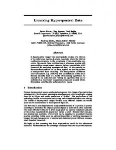
B. Notation An order-P tensor T P RN1 ˆ¨¨¨ˆNP (P ą 2) is an N1 ˆ ¨ ¨ ¨ ˆ NP array with elements indexed by T n1 ,n2 ,...,nP . The P dimensions of a tensor are called modes. A mode` fiber of tensor T is the one-dimensional subset of T obtained by fixing all but the `-th dimension, and is indexed by T n1 ,...,n`´1 ,:,n``1 ,...,nP . A slab or slice of tensor T is a two-dimensional subset of T obtained by fixing all but two of its modes. An HI is often conceived as a three dimensional data cube, and can be naturally represented by an order-3 tensor R P RN1 ˆN2 ˆL , containing N1 ˆ N2 pixels represented by the tensor fibers Rn1 ,n2 ,: P RL . Analogously, the abundances can also be collected in an order-3 tensor A P RN1 ˆN2 ˆR . Thus, given a pixel Rn1 ,n2 ,: , the respective abundance vector αn1 ,n2 is represented by the mode-3 fiber An1 ,n2 ,: . Similarly, the endmember matrices for each pixel can be represented as an order-4 tensor M P RN1 ˆN2 ˆLˆR , where Mn1 ,n2 ,:,: “ M n1 ,n2 . We now review some operations of multilinear algebra (the algebra of tensors) that will be used in the following sections (more details can be found in [25]). C. Tensor product definitions Definition 1. Outer product: The outer product between vectors bp1q P RN1 , bp2q P RN2 , . . . , bpP q P RNP is defined as the order-P tensor T “ bp1q ˝ bp2q ˝ ¨ ¨ ¨ ˝ bpP q P RN1 ˆN2 ˆ¨¨¨ˆNP , p1q p2q pP q piq where T n1 ,n2 ,...,nP “ bn1 bn2 ¨ ¨ ¨ bnP and bni is the ni -th position of bpiq . It generalizes the outer product between two vectors. Definition 2. Mode-k product: The mode-k product, denoted U “ T ˆk B, of a tensor T P RN1 ˆ¨¨¨ˆNk ˆ¨¨¨ˆNP and a matrix B P RMk ˆNk is evaluated such that each mode-k fiber of T is multiplied by matrix B, yielding U n1 ,n2 ,...,mk ,...,nP “ řNk i“1 T ...,nn´1 ,i,nn`1 ,... B mk ,i . Definition 3. Multilinear product: The full8multilinear prod0 uct, denoted by T ; B p1q , B p2q , . . . , B pP q , consists of the successive application of mode-k products between T and matrices B piq , represented as T ˆ1 B p1q ˆ2 B p2q ˆ3 . . .ˆP B pP q . Definition 4. Mode-(M,1) contracted product: The contracted mode-M product, denoted by U “ T ˆM b, is a product between a tensor T and a vector b in mode-M, where the resulting ř singleton dimension is removed, given by Nn U ...,nn´1 ,nn`1 ,... “ i“1 T ...,nn´1 ,i,nn`1 ,... bi . D. The Canonical Polyadic Decomposition An order-P rank-1 tensor is obtained as the outer product of P vectors. The rank of an order-P tensor T is defined as the minimum number of order-P rank-1 tensors that must be added to obtain T [15]. Thus, any tensor T P RN1 ˆN2 ˆ¨¨¨ˆNP with rankpT q “ K can be decomposed as a linear combination of at least K outer products of P rank-1 tensors. This socalled polyadic decomposition is illustrated in Figure 1. When this decomposition involves exactly K terms, it is called the canonical polyadic decomposition (CPD) [25] of a rank-K tensor T , and is given by

T “

K ÿ

p1q

λ i bi

p2q

˝ bi

pP q

˝ ¨ ¨ ¨ ˝ bi

.

(3)

i“1

It has been shown that this decomposition is essentially unique under mild conditions [15]. The CPD can be written alternatively using mode-k products as T “ D λ ˆ1 B p1q ˆ2 B p2q ¨ ¨ ¨ ˆP B pP q

(4)

or using the full multilinear product as 8 0 (5) T “ D λ ; B p1q , B p2q , . . . , B pP q ` ˘ where D λ “ DiagP λ1 , . . . , λK is the P -dimensional dippq ppq agonal tensor and B ppq “ rb1 , . . . , bK s, for p “ 1, . . . , P . N1 ˆN2 ˆ¨¨¨ˆNP Given a tensor T P R , the CPD can be obtained by solving the following optimization problem [15] ´ ¯ p λ ,B p p1q , . . . , B p pKq “ D arg min D λ ,B p1q ,...,B pKq

K ›2 (6) ÿ 1 ›› p1q pP q › λ i bi ˝ ¨ ¨ ¨ ˝ bi › . ›T ´ 2 F i“1

A widely used strategy to compute an approximate solution to (6) is to use an alternating least-squares technique [15], which optimizes the cost function with respect to one term at a time, while keeping the others fixed, until convergence. Although optimization problem (6) is generally non-convex, its solution is unique under relatively mild conditions, which is an important advantage of tensor-based methods [15].

E. Tensor rank bounds Finding the rank of an arbitrary tensor T is NP-hard [26]. In [15], upper and lower bounds on tensor ranks are presented for arbitrary tensors. Let T be an order-3 tensor and R1 ” dim spantT :,j,k u@j,k R2 ” dim spantT i,:,k u@i,k

(7)

R3 ” dim spantT i,j,: u@i,j be the mode-1 (column), mode-2 (row) and mode-3 (fiber) ranks, respectively, of T . Thus, the K ” rankpT q which is able to represent an arbitrary tensor is limited in the interval maxpR1 , R2 , R3 q ď K ď minpR1 R2 , R1 R3 , R2 R3 q.

(8)

The reader can note that the bounds presented above often lead to very large tensor ranks. In many practical applications, however, the “useful signal” rank is often much less than the actual tensor rank [15]. Hence, when low-rank decompositions are employed to extract low-dimensional structures from the signal, the ranks that lead to meaningful results are usually much smaller than maxpR1 , R2 , R3 q. In Section III-E, we propose a strategy to estimate the rank of tensor CPDs based on the variation of the multilinear singular values of T .

4

Fig. 1: Polyadic decomposition of a three-dimensional tensor, written as both outer products and modeń products.

III. L OW- RANK U NMIXING P ROBLEM An effective strategy to capture the low-dimensional structures of HIs for solving the HU problem is to impose a lowrank structure to the abundance tensor [22]. The same strategy can also be applied to the endmember tensor if one considers the endmember variabilities to be small or highly correlated in low-dimensional structures within the HI. Thus, assuming that A has a low-rank KA , and that M has a low-rank KM the global cost functional for the unmixing problem can be written as JpA,Mq “ N N 1 ÿ1 ÿ2 2n

1 “1

To solve (11), we propose to find a local stationary point by minimizing (10) iteratively with respect to each variable. The resulting algorithm is termed the Unmixing with Lowrank Tensor Regularization Algorithm accounting for spectral Variability (ULTRA-V), and is presented in Algorithm 1. The intermediate steps are detailed in the following. Algorithm 1: Global algorithm for solving (10)

6

Input : R, λM , λA , Ap0q , and Mp0q . x Output: Ap and M. KQ = esitmateTensorRank(Ap0q ); KP = esitmateTensorRank(Mp0q ); Set i “ 0 ; while stopping criterion is not satisfied do i“i`1 ; P piq “ arg min JpApi´1q , Mpi´1q , Pq ;

7

Qpiq “ arg min JpApi´1q , Mpi´1q , Qq ;

8

Mpiq “ arg min JpApi´1q , M, P piq , Qpiq q ;

9

Apiq “ arg min JpA, Mpiq , P piq , Qpiq q ;

1 2

}Rn1 ,n2 ,: ´ Mn1 ,n2 ,:,: An1 ,n2 ,: }2F

n2 “1

3

(9)

s. t. rankpMq “ KM , M ľ 0

4 5

P

1

rankpAq “ KA , A ľ 0, A ˆ 1R “ 1N1 ˆN2 .

P

Defining the HU problem as in (9) with fixed data independent ranks KM and KA limits its flexibility to adequately represent the desired abundance maps and endmember variability. Though fixing low ranks for A and M tends to capture the most significant part of the tensors energy [27], one may incur in a loss of fine and small scale details that may be relevant for specific data. On the other hand, using large values for KA and KM makes the solution sensitive to noise, undermining the purpose of regularization. Thus, an important issue is how to effectively impose the low-rank constraint to achieve regularity in the solution without undermining its flexibility to adequately model small variations and details. We propose to modify (9) by introducing new regularization terms, controlled by two low-rank tensors Q P RN1 ˆN2 ˆR and P P RN1 ˆN2 ˆLˆR , to impose non-strict constraints on KA and KM . Doing that, tensors Q and P work as a priori information, and the strictness of the low-rank constraint is controlled by two additional parameters λA , λM P R` . The proposed cost function is given by JpA,M, P, Qq “ N N 1 ÿ1 ÿ2 }Rn1 ,n2 ,: ´ Mn1 ,n2 ,:,: An1 ,n2 ,: }2F 2 n “1 n “1 1

2

(10)

λM λA }M ´ P}2F ` }A ´ Q}2F 2 2 s. t. M ľ 0, A ľ 0, A ˆ1 1R “ 1N1 ˆN2

11

end x “ Mpiq ; return Ap “ Apiq , M

A. Solving with respect to A To solve problem (11) with respect to A we use only the terms in (10) that depend on A, leading to the cost function JpAq “

N N 1 ÿ1 ÿ2 }Rn1 ,n2 ,: ´ Mn1 ,n2 ,:,: An1 ,n2 ,: }2F 2 n “1 n “1 1

2

λA ` }A ´ Q}2F 2 s. t. A ľ 0, A ˆ1 1R “ 1N1 ˆN2

(12)

which results in a standard regularized fully constrained leastsquares problem that can be solved efficiently.

Analogously to the previous section, to solve problem (11) with respect to M, we use only the terms in (10) that depend on M, leading to JpMq “

with rankpPq “ KM and rankpQq “ KA . The optimization problem becomes A,M,P,Q

A

10

B. Solving with respect to M

`

p M, x P, p Qq p “ arg min JpA, M, P, Qq. pA,

M

(11)

N N 1 ÿ1 ÿ2 }Rn1 ,n2 ,: ´ Mn1 ,n2 ,:,: An1 ,n2 ,: }2F 2 n “1 n “1 1

2

λM ` }M ´ P}2F 2 s. t. M ľ 0.

(13)

5

constant λA . Using (20) in (19) leads to the optimization problem ´ ¯ p ,Z p p1q , Z p p2q , Z p p3q “ Ξ (21)

which results in a regularized nonnegative least-squares problem. An approximate solution can be obtained ignoring the positivity constraint over the endmember tensor and projecting the least-squares result onto the positive orthant as [12] ˜ ´ ¯ x n1,n2,:,: “P` Rn1,n2,: AJ M ` λM P n1,n2,:,:

K Q ›2 ÿ λA ›› p1q p2q p3q › ξi z i ˝ z i ˝ z i › ›A ´ F Ξ,Z p1q ,Z p2q ,Z p3q 2 i“1 ` ˘ where Ξ “ Diag3 ξ1 , . . . , ξKQ is an order-3 diagonal tensor with Ξi,i,i “ ξi . Problem (21) can be solved using an alternating least-squares strategy [15]. Finally, the solution p is obtained from Ξ, p Z p p1q , Z p p2q and Z p p3q using the full Q multilinear product as 8 0 p “ Ξ p ;Z p p1q ; Z p p2q ; Z p p3q . (22) Q

arg min

n1,n2,:

¸ (14) ´ ¯´1 An1,n2,: AJ n1,n2,: ` λM I 1 ˆN1 ˆL where P` : M Ñ M` , RN1 ˆN1 ˆL Ñ RN is the ` projection operator that maps every negative element to zero.

C. Solving with respect to P Rewriting the terms in (10) that depend on P leads to

E. Estimating tensor ranks

λM }M ´ P}2F . (15) 2 Assuming that most of the energy of M lies in a low-rank structure, we write the tensor P as a sum of a small number KP of rank-1 components, such that JpPq “

P“

K P ÿ

p1q

δi xi

p2q

˝ xi

p3q

˝ xi

p4q

˝ xi .

(16)

i“1

This introduces a low-rank a priori condition on P whose strictness can be controlled by the regularization constant λP . Using (16) in (15) leads to the optimization problem ´ ¯ p1q p2q p3q p4q p X x ,X x ,X x ,X x ∆, “ (17) › ›2 K › P ÿ λM ›› p1q p2q p3q p4q › δi xi ˝ xi ˝ xi ˝ xi › arg min ›M ´ › ∆,X p1q ,X p2q ,X p3q ,X p4q 2 › i“1

F

where ∆ “ Diag4 pδ1 , . . . , δKP q is a 4 dimensional diagonal tensor with ∆i,i,i,i “ δi . Problem (17) can be solved using an alternating least-squares strategy [15]. p1q p2q p is obtained from ∆, p X x ,X x , Finally, the solution P x X

p3q

x , and X

p4q

using the full multilinear product as 0 p1q p2q p3q p4q 8 p “ ∆; p X x ,X x ,X x ,X x P .

In Section II-E we have recalled important results relating bounds for order-3 tensor ranks to the span of the matricized versions of tensors. We have also noted, from our own experience, that those bounds tend to indicate tensor ranks that are larger than the rank associated with the information relevant for HU. Our interest in HU is to model low-dimensional structures of the HI using low-rank tensors. At the same time, this low-rank representation should be rich enough to include all dimensions of the original HI tensor that contain relevant information. We propose to approximate the “useful rank” of a tensor by the number of the largest singular values of their matricized versions required to represent most of the tensor energy. Let T i “ mati pT q P RNi ˆpN1 ...Ni´1 Ni`1 ,...NP q be the matricization of an arbitrary tensor T P RN1 ˆN2 ...ˆNP obtained by stacking all tensor fibers along the i-th tensor dimension. Let si “ SVDpT i q be the set of singular values of T i , sorted descending in value. Also, let di “ diffpsi q be the vector of first order differences of the elements of si , such that, piq piq piq dj “ sj ´ sj`1 . Then, we define the i-th candidate for piq rank of T as the smallest index j such that |dj | sufficiently small, namely, ˆ i “ min j, s.t., |dpiq | ă ε R j

(18)

D. Solving with respect to Q

(23)

where ε is a parameter limiting the singular value variation. In all experiments reported here we used ε “ 0.15. Finally, we approximate the rank of tensor T as

Analogous to the previous section, the cost function to be optimized for Q can be written as

ˆ1, . . . , R ˆ P u. K “ maxtR

λA }A ´ Q}2F . (19) 2 Assuming that most of the energy of A lies in a low-rank structure, we write tensor Q as a sum of a small number KQ of rank-1 components, such that

For the experiments reported in this paper, we have used definition (24) to estimate KP and KQ in (16) and (20) from the abundance and endmember tensors estimated using simple unmixing strategies such as the scaled constrained least squares (SCLS) [11].

JpQq “

Q“

K Q ÿ

(24)

IV. S IMULATIONS p1q

ξi z i

p2q

˝ zi

p3q

˝ zi .

(20)

i“1

This introduces a low-rank a priori condition on A, which will be more or less enforced depending on the regularization

In this section, the performance of the proposed methodology is illustrated through simulations with both synthetic and real data. We compare the proposed ULTRA-V method with the the fully constrained least squares (FCLS), the scaled

6

TABLE I: Simulation results using synthetic data. Data Cube 0 – DC0

FCLS SCLS PLMM ELMM GLMM ULTRA-V

MSEA

MSEM

SAMM

MSER

SAMR

Time

1.81 0.68 1.05 0.35 0.34 0.23

175.79 88.07 106.17 101.51 92.39

6.19 5.64 5.63 5.87 5.56

16.11 59.38 4.72 4.78 5.7e-3 0.73

5.92 5.42 3.37 3.40 0.09 1.32

0.42 0.38 81.89 17.15 20.23 14.46

6.93 24.78 2.39 0.01 0.01 4.26

3.71 3.41 2.27 0.09 0.08 2.56

0.74 0.76 88.35 23.18 29.81 29.47

2.03 1.07 2.12 2.31 2.04 9e-5

13.69 12.68 12.17 13.13 12.58 0.49

0.30 0.30 61.13 11.15 11.60 5.19

Data Cube 2 – DC1 FCLS SCLS PLMM ELMM GLMM ULTRA-V

2.01 2.07 1.86 1.29 1.20 1.12


1.90 0.71 1.27 0.63 0.59 0.46

92.16 60.83 69.15 68.11 60.12

5.37 4.34 5.95 6.09 5.21

Data Cube 3 – DC2 1.66 2.45 2.84 1.84 2.91

2.29 2.28 3.32 2.79 2.94

constrained least squares (SCLS) [11], the PLMM [10], the ELMM [11], and the GLMM [12]. To measure the accuracy of the unmixing methods we consider the Mean Squared Error (MSE) MSEX “

1 p q}2 }vecpX q ´ vecpX NX

(25)

where vecp¨q is the vectorization operator X Ñ x, Raˆbˆc ÞÑ Rabc , NX “ abc, and the Spectral Angle Mapper for the HI SAMR

ˆ J ˙ N pn 1 ÿ rn r “ arccos N n“1 }r n }}p rn }

and for the endmembers tensor ˜ ¸ N R xk,n mJ 1 ÿ ÿ k,n m SAMM “ arccos . N n“1 k“1 }mk,n }}x mk,n }

(26)

(27)

A. Synthetic data For a comprehensive comparison among the different methods we created three synthetic datasets, namely Data Cube 0 (DC0), Data Cube 1 (DC1) and Data Cube 2 (DC2), with 50ˆ50 pixels (DC0 and DC2) and 70x70 pixels (DC1). DC0 and DC1 were built using three 224-band endmembers extracted from the USGS Spectral Library [28], while DC2 was built using three 16-band minerals often found in bodies of the Solar System. For the three datasets, spatially correlated abundance maps were used, as depicted in the first column of Fig. 2. For DC0, we adopted the variability model used in [11] (a multiplicative factor acting on each endmember). For DC1, we used the variability model according to the

PLMM [10]. For DC2, we used the Hapke model [29] devised to realistically represent the spectral variability introduced due to changes in the illumination conditions caused by the topography of the scene [11]. White Gaussian noise was added to all datasets to yield a 30dB SNR. In all cases, we used endmembers extracted using the VCA [30] either to build the reference endmember matrix or to initialize the different methods. The abundance maps were initialized using the maps estimated by the SCLS. To select the optimal parameters for each algorithm, we performed grid searches for each dataset. We used parameter search ranges based on the ranges tested and discussed by the authors in the original publications. For the PLMM we used γ “ 1, since the authors fixed this parameter in all simulations, and searched for α and β in the ranges r0.35, 0.7, 1.4, 25s and r10´9 , 10´5 , 10´4 , 10´3 s, respectively. For both ELMM and GLMM, we selected the parameters among the following values: λS , λM P r0.01, 0.1, 1, 5, 10, 15s, λA P r0.001, 0.01, 0.05s, and λψ , λΨ P r10´6 , 10´3 , 10´1 s, while for the proposed ULTRA-V we selected the parameters in the intervals λA P r0.001, 0.01, 0.1, 1, 10, 100s and λM P r0.1, 0.2, 0.4, 0.6, 0.8, 1s. The results are shown in Table I, were the best and second best results for each metric are marked in bold red and bold blue, respectively. ULTRA-V clearly outperformed the competing algorithms for all datasets in terms of MSEA . For the other metrics, the best results depended on the datasets. In terms of MSEM and SAMM , ULTRA-V yielded the second best result for DC0 and the best result for DC1. Finally, ULTRA-V results for MSER and SAMR were the second best for DC0 and the best for DC2. The execution

7

FCLS

SCLS

PLMM

ELMM

GLMM

ULTRA-V

Ground T.

FCLS

SCLS

PLMM

ELMM

GLMM

ULTRA-V

Ground T.

FCLS

SCLS

PLMM

ELMM

GLMM

ULTRA-V

EM #3

EM #2

EM #1

EM #3

EM #2

EM #1

EM #3

EM #2

EM #1

Ground T.

Fig. 2: Abundance maps of (top–down) DC0, DC1, and DC2 for all tested algorithms. Abundance values represented by colors ranging from blue (αk “ 0) to red (αk “ 1).

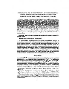
times, shown in the rightmost columns of Table I, show that ULTRA-V required the smallest execution time among the more sophisticated algorithms (PLMM, ELMM and GLMM) for DC0 and DC2, and comparable execution time for DC1. 1) Parameters sensitivity: While we have proposed a strategy to determine rank values for tensors P and Q, the parameters λM and λA need to be selected by the user. We now study the sensitivity of the ULTRA-V performance to variations of the parameters within the parameter search intervals presented in the previous section. Figure 3 shows the values of MSEA resulting from unmixing the data using each combination of the parameter values. The sensitivity clearly tends to increase when values less than 1 are used for both parameters. Our practical experience indicates that good MSEA results can be obtained using λM in r0, 1s, and large values about 100 for

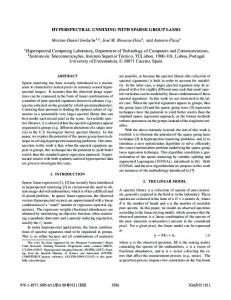
λA . Moreover, some insensitivity is verified for small changes in λA about large values. Thus, searching λA in r0.001, 100s with values spaced by decades as done for the examples in the previous section seems reasonable. B. Real data We considered the Houston and Cuprite datasets discussed in [11] for simulations with real data. Both datasets were captured by the AVIRIS, which originally has 224 spectral bands. The water absorption bands were removed resulting in 188 bands. The Houston data set is known to have four predominant endmembers while previous studies indicate the presence of at least 14 endmembers in the Cuprite mining field [30]. For both images the endmembers were extracted using the VCA [30]. Fig. 4 shows the reconstructed abundance

8

4

2 0.5

6M

00

50

100

6A

MSE

6

1

0.015

0.02

MSE

MSE

#10 -3 8

0.015

0.01 0

50

6A

100

0

0.5

1

0.01 0.005 0 1 0.5 0

6M

6M

0

50

100

6A

Fig. 3: Parameters sensitivity to changes around the optimal values. Top left: DC0, Top right: DC1, and bottom: DC2.

maps for both images and for all tested methods. Table II shows the quantitative results in terms of RMSER and SAMR . The last column in Fig. 4 shows that the proposed ULTRA-V method provided smooth and accurate abundance estimation, clearly outperforming the competing algorithms. In fact, for the Concrete and Metallic Roofs endmembers, the ULTRAV abundance map presents stronger Concrete and Metallic Roofs components in the stadium stands and stadium towers, respectively, when compared with the other methods equipped for dealing with spectral variability. Furthermore, the asphalt distribution seems more coherent. For the Cuprite Mining Field we selected four endmembers whose distribution in the scene can be clearly distinguished [30], and that were also used in [11], [31], [32]. Examining the abundance maps at the last column of Fig. 4, ULTRA-V presents smoother abundance maps for all four depicted endmembers while keeping strong components in regions where these endmembers are known to exist. The objective metrics presented in Table II indicate that ULTRA-V yields competitive reconstruction errors in terms of MSE and SAM. These results, however, should be interpreted with proper care, as the connection of reconstruction error and abundance estimation is not straightforward. The execution times in Table II indicate that ULTRA-V did not scale well with the larger image sizes and higher number of endmembers of the Cuprite data, which directly impacted the CPD stage of ULTRA-V. Moreover, the more complex images resulted in higher rank estimates using the strategy discussed in Section III-E. This indicates that there is still room for improving the proposed method by either providing a segmentation strategy or using faster CPD methods. This, however, is an open problem that will be addressed in future works. V. C ONCLUSIONS In this paper, we proposed a new low-rank regularization strategy for introducing low-dimensional spatial-spectral structure into the abundance and endmember tensors for hyperspectral unmixing considering spectral variability. The resulting iterative algorithm, called ULTRA-V, imposes lowrank structure by means of regularizations that force most of the energy of the estimated abundances and endmembers to lay within a low-dimensional structure. The proposed approach does not confine the estimated abundances and endmembers

to a strict low-rank structure, which would not adequately account for the complexity experienced in real-world scenarios. The proposed methodology includes also a strategy to estimate the rank of the regularization tensors P and Q, leaving only two parameters to be adjusted within a relatively reduced search space. Simulation results using both synthetic and real data showed that the ULTRA-V can outperform state-of-theart unmixing algorithms accounting for spectral variability. R EFERENCES [1] J. M. Bioucas-Dias, A. Plaza, G. Camps-Valls, P. Scheunders, N. Nasrabadi, and J. Chanussot, “Hyperspectral remote sensing data analysis and future challenges,” IEEE Geoscience and Remote Sensing Magazine, vol. 1, no. 2, pp. 6–36, 2013. [2] N. Keshava and J. F. Mustard, “Spectral unmixing,” IEEE Signal Processing Magazine, vol. 19, no. 1, pp. 44–57, 2002. [3] J. M. Bioucas-Dias, A. Plaza, N. Dobigeon, M. Parente, Q. Du, P. Gader, and J. Chanussot, “Hyperspectral unmixing overview: Geometrical, statistical, and sparse regression-based approaches,” IEEE Journal of Selected Topics in Applied Earth Observations and Remote Sensing, vol. 5, no. 2, pp. 354– 379, 2012. [4] N. Dobigeon, J.-Y. Tourneret, C. Richard, J. C. M. Bermudez, S. McLaughlin, and A. O. Hero, “Nonlinear unmixing of hyperspectral images: Models and algorithms,” IEEE Signal Processing Magazine, vol. 31, no. 1, pp. 82–94, Jan 2014. [5] T. Imbiriba, J. C. M. Bermudez, C. Richard, and J.-Y. Tourneret, “Nonparametric detection of nonlinearly mixed pixels and endmember estimation in hyperspectral images,” IEEE Transactions on Image Processing, vol. 25, no. 3, pp. 1136–1151, March 2016. [6] T. Imbiriba, J. C. M. Bermudez, and C. Richard, “Band selection for nonlinear unmixing of hyperspectral images as a maximal clique problem,” IEEE Transactions on Image Processing, vol. 26, no. 5, pp. 2179–2191, May 2017. [7] A. Zare and K. C. Ho, “Endmember variability in hyperspectral analysis: Addressing spectral variability during spectral unmixing,” Signal Processing Magazine, IEEE, vol. 31, p. 95, January 2014. [8] L. Drumetz, J. Chanussot, and C. Jutten, “Variability of the endmembers in spectral unmixing: recent advances,” in 8th IEEE Workshop on Hyperspectral Image and Signal Processing: Evolution in Remote Sensing, Los Angeles, USA, 2016. [9] R. A. Borsoi, T. Imbiriba, and J. C. M. Bermudez, “Super-resolution for hyperspectral and multispectral image fusion accounting for seasonal spectral variability,” arXiv preprint arXiv:1808.10072, 2018. [10] P.-A. Thouvenin, N. Dobigeon, and J.-Y. Tourneret, “Hyperspectral unmixing with spectral variability using a perturbed linear mixing model,” IEEE Trans. Signal Processing, vol. 64, no. 2, pp. 525–538, Feb. 2016. [11] L. Drumetz, M.-A. Veganzones, S. Henrot, R. Phlypo, J. Chanussot, and C. Jutten, “Blind hyperspectral unmixing using an extended linear mixing model to address spectral variability,” IEEE Transactions on Image Processing, vol. 25, no. 8, pp. 3890–3905, 2016. [12] T. Imbiriba, R. A. Borsoi, and J. C. M. Bermudez, “Generalized linear mixing model accounting for endmember variability,” in ICASSP, IEEE International Conference on Acoustics, Speech and Signal Processing, April 2018, pp. 1862–1866.

9

SCLSU

PLMM

ELMM

GLMM

ULTRA-V

FCLS

SCLS

PLMM

ELMM

GLMM

ULTRA-V

Muscov.

Budding.

Sphene

Alunite

Asphalt

Concrete

Met. Roofs Vegetation

FCLS

Fig. 4: Abundance maps of the Houston (upper panel) and Cuprite (lower panel) datasets for all tested algorithms. Abundance values represented by colors ranging from blue (αk “ 0) to red (αk “ 1). TABLE II: Real Data. Algorithm


Houston Data

Cuprite Data

MSER

SAMR

Time

MSER

SAMR

Time

0.2283 0.0037 0.0190 0.0010 1.0e-5 0.0018

5.7695 2.5361 1.6201 1.3225 0.0472 1.5043

1.90 2.04 454.90 62.66 32.26 264.71

0.0114 0.0088 0.0027 0.0025 0.0011 0.0012

2.7008 7.8559 7.6452 7.7055 7.6264 0.8487

15.90 14.09 6971.04 474.45 1326.85 2092.18

[13] M. Tao and X. Yuan, “Recovering low-rank and sparse components of matrices from incomplete and noisy observations,” SIAM Journal on Optimization, vol. 21, no. 1, pp. 57–81, 2011. [14] M. Bousse, O. Debals, and L. De Lathauwer, “A tensor-based method for large-scale blind source separation using segmentation,” IEEE Trans-

actions on Signal Processing, vol. 65, no. 2, pp. 346–358, 2017. [15] N. D. Sidiropoulos, L. De Lathauwer, X. Fu, K. Huang, E. E. Papalexakis, and C. Faloutsos, “Tensor decomposition for signal processing and machine learning,” IEEE Transactions on Signal Processing, vol. 65, no. 13, pp. 3551–3582, 2017.

10

[16] M. K.-P. Ng, Q. Yuan, L. Yan, and J. Sun, “An adaptive weighted tensor completion method for the recovery of remote sensing images with missing data,” IEEE Transactions on Geoscience and Remote Sensing, vol. 55, no. 6, pp. 3367–3381, 2017. [17] X. Zhang, G. Wen, and W. Dai, “A tensor decomposition-based anomaly detection algorithm for hyperspectral image,” IEEE Transactions on Geoscience and Remote Sensing, vol. 54, no. 10, pp. 5801–5820, 2016. [18] X. Guo, X. Huang, L. Zhang, L. Zhang, A. Plaza, and J. A. Benediktsson, “Support tensor machines for classification of hyperspectral remote sensing imagery,” IEEE Transactions on Geoscience and Remote Sensing, vol. 54, no. 6, pp. 3248–3264, 2016. [19] S. Yang, M. Wang, P. Li, L. Jin, B. Wu, and L. Jiao, “Compressive hyperspectral imaging via sparse tensor and nonlinear compressed sensing,” IEEE Transactions on Geoscience and Remote Sensing, vol. 53, no. 11, pp. 5943–5957, 2015. [20] L. Zhang, L. Zhang, D. Tao, and X. Huang, “Tensor discriminative locality alignment for hyperspectral image spectral–spatial feature extraction,” IEEE Transactions on Geoscience and Remote Sensing, vol. 51, no. 1, pp. 242–256, 2013. [21] M. A. Veganzones, J. E. Cohen, R. C. Farias, J. Chanussot, and P. Comon, “Nonnegative tensor cp decomposition of hyperspectral data,” IEEE Transactions on Geoscience and Remote Sensing, vol. 54, no. 5, pp. 2577–2588, 2016. [22] Y. Qian, F. Xiong, S. Zeng, J. Zhou, and Y. Y. Tang, “Matrix-vector nonnegative tensor factorization for blind unmixing of hyperspectral imagery,” IEEE Transactions on Geoscience and Remote Sensing, vol. 55, no. 3, pp. 1776–1792, 2017. [23] T. Imbiriba, R. A. Borsoi, and J. C. M. Bermudez, “A low-rank tensor regularization strategy for hyperspectral unmixing,” IEEE Statistical Signal Processing Workshop, pp. 373 – 377, 2018. [24] L. De Lathauwer, B. De Moor, and J. Vandewalle, “A multilinear singular value decomposition,” SIAM journal on Matrix Analysis and Applications, vol. 21, no. 4, pp. 1253–1278, 2000. [25] A. Cichocki, D. Mandic, L. De Lathauwer, G. Zhou, Q. Zhao, C. Caiafa, and H. A. Phan, “Tensor decompositions for signal processing applications: From two-way to multiway component analysis,” IEEE Signal Processing Magazine, vol. 32, no. 2, pp. 145–163, 2015. [26] J. H˚astad, “Tensor rank is np-complete,” Journal of Algorithms, vol. 11, no. 4, pp. 644–654, 1990. [27] S. Mei, J. Hou, J. Chen, L. P. Chau, and Q. Du, “Simultaneous spatial and spectral low-rank representation of hyperspectral images for classification,” IEEE Transactions on Geoscience and Remote Sensing, vol. PP, no. 99, pp. 1–15, 2018. [28] R. N. Clark, G. A. Swayze, K. E. Livo, R. F. Kokaly, S. J. Sutley, J. B. Dalton, R. R. McDougal, and C. A. Gent, “Imaging spectroscopy: Earth and planetary remote sensing with the usgs tetracorder and expert systems,” Journal of Geophysical Research: Planets, vol. 108, no. E12, 2003. [29] B. Hapke, “Bidirectional reflectance spectroscopy, 1, Theory,” Journal of Geophysical Research, vol. 86, no. B4, pp. 3039–3054, 1981. [30] J. M. P. Nascimento and J. M. Bioucas-Dias, “Vertex Component Analysis: A fast algorithm to unmix hyperspectral data,” IEEE Transactions on Geoscience and Remote Sensing, vol. 43, no. 4, pp. 898–910, April 2005. [31] R. A. Borsoi, T. Imbiriba, J. C. M. Bermudez, and C. Richard, “Tech report: A fast multiscale spatial regularization for sparse hyperspectral unmixing,” arXiv preprint arXiv:1712.01770, 2017. [32] R. A. Borsoi, T. Imbiriba, Bermudez, and J. C. M., “A data dependent multiscale model for hyperspectral unmixing with spectral variability,” IEEE Trans. on Image Processing (Submitted), 2018.