Low-rate LDPC Convolutional Codes with Short Constraint Length Marco Baldi, Senior Member, IEEE and Giovanni Cancellieri, Member, IEEE Abstract: We study a family of LDPC convolutional codes having code rate of the type 1/a, and analyze their minimum distance and local cycles length properties. We consider some low weight codewords that are known from the literature, and are easily obtained from the symbolic parity-check matrix of these codes. Starting from the structure of such codewords, we follow a twofold approach: i) we exploit graph-based techniques to design these codes with the aim to maximize their minimum distance while keeping the syndrome former constraint length as small as possible and ii) we provide a simple form for their generator matrices that allows to perform exhaustive searches through which we verify that the code design actually reaches its target. We also estimate the normalized minimum distance multiplicity for the codes we consider, and introduce the notion of symbolic graphs as a new tool to study the code properties. Index terms: Error correcting codes, LDPC convolutional codes, Minimum distance, Spatially coupled LDPC codes, Symbolic graphs, Syndrome former constraint length.
I. INTRODUCTION LDPC convolutional codes and, more in general, spatially coupled LDPC codes are receiving special consideration in recent literature as they are able to outperform classical LDPC block codes both in the asymptotic and finite length regimes (see [1, 2] and the references therein for a detailed review). However, LDPC convolutional codes with good performance typically exhibit a rather long constraint length, with respect to traditional convolutional codes [1]. This leads to large window sizes in sliding-window decoding, which is the typical decoder operating mode for convolutional codes. Concerning performance, LDPC codes are usually decoded through iterative decoders based on the belief propagation principle, whose capacity achieving performance depends on the low density of the code parity-check matrix. On the other hand, a large minimum distance d can be obtained by increasing the column weights of the parity-check matrix, but this deteriorates the waterfall performance of the decoder and increases the decoding complexity. So, a good trade-off is to keep the average parity-check matrix column weight rather small (e.g., not greater than 4). LDPC convolutional codes can be designed by starting from quasi-cyclic (QC) LDPC block codes, through unwrapping techniques [3, 4]. In doing this, attention is mainly devoted to minimize the size of the circulant matrices forming the paritycheck matrix of the QC block code. The constraint length of the convolutional codes so obtained is influenced by this fact. Authors are with the Università Politecnica delle Marche, Ancona, Italy (e-mail:
[email protected],
[email protected])
Alternatively, LDPC convolutional codes can be designed directly, e.g., by studying and assigning the vertical separations between each pair of ones in their syndrome former matrix. This approach has already been followed by the authors in [5, 6], with focus on high rate codes. In this paper, we instead consider some families of low-rate LDPC convolutional codes, and show that their constraint length can be maintained small, while achieving large free distance. With reference to a convolutional code whose period is a, the code rate 1/a is taken into account. The codes are designed by starting from a special class of symbolic matrices H(x), which allow to straightforwardly derive the codes generator matrix, which in turn helps to analyze the code free distance d and the relevant normalized multiplicity B(d). As a first step, we define some upper bounds on d. Practical rules to verify the row-column constraint [7] are introduced as well. The goal of maintaining the syndrome former constraint length mh as small as possible is also taken into account. The form of the matrix H(x) we propose is as follows: two columns with just one polynomial each, with whichever weight, in different rows, and a series of (a − 2) columns made by two monomials in a staircase structure. This simple form allows to: i) satisfy the row-column constraint, ii) minimize the syndrome former constraint length and iii) achieve large values of the free distance d while keeping the average column weight rather small. This kind of matrices also admit an easy representation in terms of suitable graphs, denoted as symbolic graphs, which will be described in the following. The paper is organized as follows. In Section II, the design and optimization of the code polynomials is described. In Section III, we introduce the graph-based representation of the codes and the relevant properties resulting from it. We also sketch an approach to design codes having higher rates. Section IV provides some conclusive remarks. II. DESIGN OF LOW-RATE CODES Let us consider the polynomial parity-check matrix H(x) of an LDPC convolutional code, whose period contains a bits, the first of which is an information bit and the last (a – 1) bits are redundancy bits. The polynomial parity-check matrix has (a – 1) rows and a columns, and can be represented as follows:
h12 ( x) ⎡ h11 ( x) ⎢ h ( x) h22 ( x) 21 H(x) = ⎢ ⎢ ... ⎢ h ( x ) h ( x ) ( a −1)2 ⎣⎢ ( a −1)1
h1a ( x) ⎤ h2 a ( x) ⎥⎥ ⎥ ⎥ h( a −1)a ( x) ⎦⎥
(1)
where the polynomials
hij ( x)
are named input-output
polynomials with reference to an encoder in observer canonical form. An upper bound on the free distance can be obtained by considering some unavoidable codewords, as discussed in some recent literature on LDPC convolutional codes [4]. According to this approach, we adopt the following structure for H(x):
⎡ p ( x) ⎢ ⎢ 0 ⎢ 0 H(x) = ⎢ ⎢ ⎢ 0 ⎢ ⎢⎣ 0
1 1 0
0 1 1
0 0
0 0
0 0 1 ... 0 0
... ... ... ... ... ...
0 0 0 1 0
⎤ ⎥ ⎥ ⎥ ⎥ ⎥ 1 0 ⎥ ⎥ 1 q ( x) ⎥⎦ 0 0 0
0 0 0
polynomial products appearing in (4). Avoiding both such situations is a necessary condition for the free distance to reach the bound (5). We suppose that both the polynomials p(x) and q(x) exhibit a non-null 0.th-order coefficient. Therefore, the following relationship holds between the syndrome former constraint length mh and the degrees of the two polynomials mh = max{deg[p(x)], deg[q(x)]}
(2)
where p(x) and q(x) are suitable polynomials with weights wp and wq respectively (the weight of a polynomial is defined as
(6)
Let us consider codes with rate 1/2, 1/3 and 1/4 (that is, a = 2, 3, 4) and some small values of wp and wq (not greater than 4 and 3, respectively). We have analyzed all the possibilities for p(x) and q(x), with the aim to find those solutions which maximize the weight of t(x) expressed by (4). Table I. Polynomial weights, average weight, maximum free distance d and minimum syndrome former constraint length mh for code rates 1/2, 1/3 and 1/4.
the number of its non-zero coefficients). The average column weight of the parity-check matrix of this family of codes turns out to be
w =
wp + wq + 2 ( a − 2 ) a
(3)
According to [4, 8], the code defined by H(x) as in (2) contains a codeword whose polynomial expression is
t(x) = ⎡⎣ q * ( x )
p * ( x ) q * ( x ) ...
p *( x) q *( x)
p * ( x ) ⎤⎦ (4)
where * denotes the reciprocal polynomial. A straightforward upper bound on this codeword weight follows from its definition, and it also provides an upper bound on the code free distance d, that is, d ≤ w p + wq + ( a − 2 ) w p wq
(5)
The symbolic generator matrix G(x), consisting of only one row, can be obtained by eliminating possible common factors among the a polynomials forming t(x) in (4), and can be used to generate any codeword through multiplication by the corresponding information polynomial. So, the free distance d and the normalized minimum distance multiplicity B(d) can be estimated by performing an exhaustive search based on the generator matrix so obtained. This procedure is feasible since the constraint lengths of these codes are rather small. Concerning the choice of the coefficients of p(x) and q(x), we should take into account the following constraints. Let us consider, in each polynomial, all the differences between any two powers of x having a non-zero coefficient. If, in one or both polynomials, any difference appears twice, then the rowcolumn constraint is not met. Two equal differences, one in p(x) and the other in q(x), do not allow reaching the bound (5) with the equality sign. The last observation follows from the weight lowering effect that is due to collisions in the central
Table II. Polynomials p(x) and q(x) able to achieve the maximum possible free distance d with minimum mh , and corresponding normalized minimum distance multiplicity B(d)
In Table I we provide the results of this analysis. The table
columns respectively collect the weights of the two polynomials, the average column weight of H(x), the code period a and the code rate 1/a. The smallest value of mh allowing to achieve the bound (5) with the equality sign is also reported. We observe that the values of mh so obtained are rather small, in spite of the high free distance which they allow to reach. The optimal solutions for p(x) and q(x) we have found for each case are provided in Table II, together with the values of B(d) computed through the aforementioned exhaustive search. We observe that such values are indeed very small. In fact, we usually obtain B(d) = 1, except in two cases for which B(d) = 2. The possible occurrence of codewords with the form (4), but with weight smaller than the r.h.s. term of (5), can be avoided by exploiting a suitable graph representation of these codes, which will be described in the next Section. III. DESCRIPTION BY MEANS OF SYMBOLIC GRAPHS LDPC block and convolutional codes can be described through their parity-check matrices or, alternatively, through the well-known bipartite graphs called Tanner graphs [7]. A closed path starting from one node of the graph and returning to the same node is called a cycle. A detrimental feature for the code properties and the LDPC decoder performance is the presence of short cycles in the Tanner graph of a code. For regular LDPC codes with parity-check matrices having column weight 2, a cycle in the Tanner graph also corresponds to a codeword. In fact, it is easy to verify that the columns of the parity-check matrix associated to the variable nodes included in the cycle sum to zero. Hence, a codeword exists with support indexes corresponding to the indexes of those columns [9]. The weight of such a codeword is half the length of the corresponding cycle. Therefore, in this case the presence of short cycles in the Tanner graph also implies a small minimum distance of the code. This is generally true also for codes having parity-check matrices with higher column weights, even though such a direct relationship between these two features of a code no longer exists. For the LDPC convolutional codes we consider, cycles in the Tanner graph can also be described based on some smaller, directed weighted graphs we denote as symbolic graphs (since they correspond to the symbolic representation of the paritycheck matrices, and their edges may have weights greater than 1, differently from Tanner graphs). Each symbolic graph has as many nodes as the (a – 1) redundancy symbols per period and a edges. The type of nodes and edges in a symbolic graph varies according to the entries of H(x) and, more precisely, to the weight of the polynomials that form the entries of H(x). An edge connecting two nodes of a symbolic graph corresponds to a pair of monomials in one column of H(x), whereas a closed loop in a symbolic graph starting from and returning to some node corresponds to a binomial in one column of H(x). The presence of polynomials having weights greater than 2 introduces some more complex nodes in the symbolic graphs. More precisely, each polynomial with weight w > 2 corresponds to a node in the symbolic graph having w inner states, and an edge may connect any two of these states. This
indeed occurs also for binomials, but for the sake of simplicity, the two states corresponding to a binomial are condensed into a unique symbol, and the edge connecting them is transformed into a closed loop. When searching for closed paths in these graphs, we can move among the inner states of a node through the graph edges or even directly, i.e., without passing through any edge. The label of the j-th edge in a symbolic graph reports its weight, denoted by bj. Its value coincides with the vertical separation between non-zero symbols in the syndrome former sub-matrix corresponding to the polynomials associated to that edge. These values can be easily computed by starting from the syndrome former sub-matrix of a code. This procedure will be described in detail in Section III.A, through an example. Alternatively, simple formulas can be written to start from a polynomial (or a pair of polynomials) and obtain their corresponding values bj. Each edge has weight bj when it is considered in one direction (the main direction, indicated in the graph), while it has weight –bj when it is considered in the opposite direction. A short cycle in the code Tanner graph corresponds to a closed path in the symbolic graph having a cumulative edge weight equal to zero. The length of the cycle in the Tanner graph is twice the length of the closed path with null cumulative edge weight in the symbolic graph. Each symbolic graph contains an unavoidable closed path, which is obtained by considering all the edges in both directions. A. Computing the symbolic graph of a code Let us consider a time-invariant LDPC convolutional code with a = 4 (i.e., code rate 1/4) defined by the following syndrome former matrix:
⎡1 0 0 1 0 0 0 0 0 0 0 0 0 0 0 0 0 0 0 0 0 1 0 0 ⎤ ⎢1 1 0 0 0 0 0 0 0 0 0 0 0 0 0 0 0 0 0 0 0 0 0 0 ⎥ ⎥ (7) H0 = ⎢ ⎢0 1 1 0 0 0 0 0 0 0 0 0 0 0 0 0 0 0 0 0 0 0 0 0 ⎥ ⎥ ⎢ ⎣0 0 1 0 0 0 0 0 0 0 0 1 0 0 0 0 0 1 0 0 0 0 0 0 ⎦ The transpose of this matrix, H0T, is the main component of the semi-infinite parity-check matrix H of the LDPC convolutional code, which therefore is defined by H0. More precisely, H is formed by infinite repetitions of H0T along its main diagonal, and zeros elsewhere. Each repetition of H0T is shifted down by a number of rows equal to the number of redundancy bits per period r0. For the codes we consider, we have r0 = a – 1 = 3. An alternative representation of H0 is based on the positions of the non-zero symbols along its rows. In fact, by considering such indexes, we can describe the matrix in (7) through the following multiset:
⎧{0,3, 21} ⎪ ⎪{0,1} I0 = ⎨ ⎪{1, 2} ⎪{2,11,17} ⎩
(8)
The symbolic parity-check matrix H(x) is easily obtained from I0. In fact, H(x) has r0 rows and a columns. Each column of H(x) corresponds to one set in I0. The values in the set must be compared with r0 in order to determine their corresponding polynomials in H(x). More precisely, their value computed modulo r0 determines the row of the corresponding polynomial (the rows of H(x) are counted starting from zero), while the integer division of their values by r0 determines the exponents of x in their corresponding polynomials. We use negative exponents of x as a convention, but positive exponents could be used as well. So, if we consider the first set in I0 as in (8), we have that the corresponding rows of H(x) are {0, 3, 21} mod 3 = {0, 0, 0} and the corresponding exponents of x are {0, 3, 21} div 3 = {0, 1, 7}. If we consider the second set, we have that the corresponding rows of H(x) are {0, 1} mod 3 = {0, 1} and the corresponding exponents of x are {0, 1} div 3 = {0, 0}. Similarly, the third set in I0 corresponds to the rows of H(x) at positions {1, 2} mod 3 = {1, 2} and the exponents of x equal to {1, 2} div 3 = {0, 0}. Finally, the last set in I0 corresponds to the rows of H(x) at positions {2, 11, 17} mod 3 = {2, 2, 2} and the exponents of x equal to {2, 11, 17} div 3 = {0, 3, 5}. Based on this procedure, we obtain the following symbolic parity-check matrix for the considered code: ⎡( x −7 + x −1 + 1) 1 ⎤ ⎢ ⎥ 1 1 H(x) = ⎢ ⎥ ⎢ 1 ( x −5 + x −3 + 1) ⎥⎦ ⎣
(9)
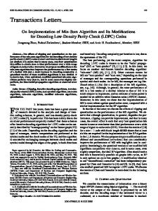
Starting from (7), (8) and (9), it is easy to obtain the symbolic graph associated to this code, which is reported in Fig. 1, and explained next.
Fig. 1. Symbolic graph describing the code corresponding to (7), (8) and (9).
We have a – 1 = 3 states in the symbolic graph, as many as the redundancy bits per period added by the convolutional
code, and the rows of the symbolic parity-check matrix (9). The first and the last rows in (9) include trinomials, therefore their corresponding nodes in the symbolic graph have three inner states each. All the possible connections among them are included as edges in the symbolic graph. The second row, instead, only includes monomials, therefore its corresponding node has a unique inner state. If we have two or more nonzero entries in the symbolic parity-check matrix at the same column, then we have one or more edges in the symbolic graph connecting two different nodes. In (9), this occurs at the second and third columns, corresponding to transitions from the state 0 to the state 1 and from the state 1 to the state 2, respectively. The weights of the symbolic graph edges are easily obtained from I0 in (8). In fact, they coincide with the differences between each pair of entries in each subset within I0. The polynomial codeword t(x) defined by (4) can be easily computed for this code. It has weight 24 and its vector of coefficients is t = [1 1 1 1 0 1 1 1 0 0 0 0 1 1 1 0 0 1 1 0 1 1 1 0 0 1… 1 0 0 1 1 1 0 0 0 0 0 0 0 0 0 1 1 0 0 0 0 0 0 1 1 0]
(10)
Since there are no common factors in the four polynomials forming the codeword t(x), the latter can be used as a symbolic generator matrix of our code. So, the vector t given by (10) coincides with the code sub-generator matrix, and allows to perform an exhaustive search of low weight codewords. This way, we have verified that this code has free distance d = 24 and normalized minimum weight multiplicity B(d) = 1. This is a good result, since a regular code based on monomials with parity-check matrix column weight 3 has free distance ≤ 24 according to [3, Theorem 3]. Our code achieves free distance equal to 24 (and the lowest possible normalized minimum weight multiplicity) with a sparser parity-check matrix (having average column weight 2.5). In addition, the syndrome former constraint length is mh = 7, which is very small, thus yielding low decoding complexity. For the sake of comparison, we observe that two codes having the same rate and free distance are reported in [10, Tables III and V], but they have mh = 21 and mh = 33, respectively. B. Using symbolic graphs to compute the minimum distance As a further example, we provide in Fig. 2 the symbolic graphs associated to the first three codes in Table II. Also in this case, the nodes are labelled as the rows of H(x) they represent. These three codes are regular with parity-check matrix column weight 2, therefore each cycle in their Tanner graph corresponds to a low weight codeword. The unavoidable closed paths with zero cumulative edge sum contained in these symbolic graphs are independent of the choice of p(x) and q(x), and therefore provide upper bounds on d for this family of codes. Nevertheless, for some special choices of p(x) and q(x), some shorter cycles may arise in the Tanner graphs of these codes. Such cycles correspond to closed paths in the symbolic graphs involving a smaller number of edges with respect to the unavoidable closed path. In order to reach the upper bound on d, such particular choices of p(x) and q(x) yielding to shorter closed paths in the
cycles as the covering of the Tanner graph variable nodes corresponding to the small weight codeword support. In other terms, we could consider separately any pair of symbols one in each column of the parity-check matrix, and study the short cycles in the Tanner graph involving their corresponding edges. This way, the analysis performed for regular codes with parity-check matrix column weight 2 can be reused. If all of such “weight-2 component codes” have only maximum-length short cycles, leading to unavoidable low-weight codewords, than the upper bound on d is reached also for the overall code. Let us denote by C the number of short cycles in the Tanner graph involving each edge corresponding to a symbol one in a column of H at a position which is in the support of a low weight codeword. The following cases may occur: C = 1 when both wp and wq are even, C = 2 when one of them is even
symbolic graphs must be avoided.
and the other is odd, C = 4 when both wp and wq are odd. We have heuristically observed that, for the codewords t(x) of the cases considered in this paper, the total number N of involved short cycles and the parameter C can be related one each other as follows: Fig. 2. Symbolic graphs describing the first three codes in Table II 9
N =C
w p wq 2 2
(11)
3 6
In Fig. 4 we provide some examples. They refer to codes having code rate 1/3, with fixed parameters C, N, wp , wq
6 2 4
3
1
1 2
1
1
(independently of the code rate). It must be said that this kind of analysis only regards the low-weight codewords of the type (4). Some other codewords with low weight and different form may arise, and this shall be avoided on a case-by-case basis.
4
⎡⎣ ( x −3 + x −2 + 1) ( x −4 + 1) ⎤⎦
8
15
⎡( x −3 + x −2 + 1) 1 ⎤ ⎢ ⎥ 1 ( x −4 + 1) ⎦ ⎣
⎡( x −3 + x −2 + 1) 1 ⎤ ⎢ ⎥ 1 1 ⎢ ⎥ −5 ⎢ ⎥ + 1 ( x 1) ⎣ ⎦
Fig. 3. Symbolic graphs describing the fourth, fifth and sixth codes in Table II
As another example, we provide in Fig. 3 the symbolic graphs associated to the fourth, fifth and sixth code reported in Table II. Differently from the case of regular codes with parity-check matrix column weight 2, in this case a short cycle in the Tanner graph does not correspond to a low weight codeword. However, it is possible to verify that low weight codewords arise from the combination of multiple short cycles in the code Tanner graph. In particular, we have observed that the bit positions in the support of a low weight codeword correspond to variable nodes in the Tanner graph which are involved in a fixed number of short cycles. We denote such a number of short
Fig. 4. Parameters N and C for some examples of codes with a = 3
Nevertheless, the existence of codewords with smaller weight still depends on the existence of closed paths with zero cumulative edge sum in the symbolic graph, and this kind of paths may become longer as the number (a – 1) of redundancy symbols per period increases. For example, the second code in Fig. 3 admits the following zero cumulative edge weights: 2+2–4=0 2+6–1–8+1=0 4+4–1+8+1=0
object of future works. The first of the corresponding closed paths is associated to a length-6 cycle in the Tanner graph, the other two are associated to length-10 cycles in the Tanner graph, whereas the unavoidable maximum-length short cycle in this case has length 16. In spite of this fact, the free distance remains d = 11 for this code. The analysis developed so far is devoted to codes having code rate 1/a. If we add further columns in H(x), e.g., with pairs of monomials, then the topology of the graph changes and many further closed paths can arise. For instance, we report in Fig. 5 the symbolic graph associated to a code having code rate 6/10 and all weight-2 columns in its parity-check matrix. All the possible dispositions of pairs of symbols one have been considered, leading to a complete mesh. Furthermore, we have four binomials, one per each row of H(x). This code is characterized by the upper bound d ≤ 8 , but mh and the normalized minimum distance multiplicity B(8) become rather high. In fact, several closed paths can be identified in its symbolic graph, and a suitable choice of the code parameters is necessary in order to avoid that they correspond to zero cumulative edge weights.
b1
0
b2
b3
ba −1
… 1 ba Fig. 6. Symbolic graph for a code with rate ( a − 2 ) a
IV. CONCLUSIONS We studied a class of low-rate LDPC convolutional codes with the goal of giving bounds on their free distance d, syndrome former constraint length mh and normalized multiplicity of minimum-weight codewords B(d). The tools used in this analysis are based on a polynomial approach and the new concept of symbolic graphs. High values of d have been demonstrated to be attainable, with B(d) as small as a few units and constraint length comparable with that of traditional (non-LDPC) convolutional codes. REFERENCES [1]
Fig. 5. Symbolic graph for a code with rate 6/10 and all weight-2 columns in its parity-check matrix H
If all the four binomials are replaced by as many trinomials, the minimum distance can increase remarkably. Nevertheless, mh becomes very high if one tries to maximize the free distance d. Furthermore, when the rows of H(x) are less than (a – 1), the symbolic generator matrix contains more than one row. The exhaustive search of low-weight codewords becomes more involved, and the approach here presented may become unfeasible. An alternative solution to design high rate codes could be to allow, in the symbolic graph, the presence of more than one edge connecting the same couple of nodes. This way, we can avoid that the number of redundancy symbols increases with a. As an example, Fig. 6 reports the symbolic graph corresponding to an LDPC convolutional code with period a and two redundancy bits per period, i.e., having code rate ( a − 2 ) a . These possible solutions to design higher rate LDPC convolutional codes and their optimization will be the
A.E. Pusane, R. Smarandache, O. Vontobel, and D.J. Costello “Deriving good LDPC convolutional codes from LDPC block codes”, IEEE Trans. Inf. Theory, vol. 57, no. 2, pp. 835-857, 2011. [2] D. G. M. Mitchell, M. Lentmaier and D. J. Costello, “Spatially Coupled LDPC Codes Constructed from Protographs”, IEEE Trans. Inf. Theory, 2015, in press. [3] I.E. Bocharova, F. Hug, R. Johannesson, B.D. Kudryashov, and R.V. Satyukov, “New low-density parity-check codes with large girth based on hypergraphs”, Proc. IEEE ISIT 2010, pp. 819-823, Austin, Texas, USA, June 2010. [4] R. Smarandache, and P.O. Vontobel, “Quasi-cyclic LDPC codes: influence of proto- and Tanner-graph structure on minimum Hamming distance upper bounds”, IEEE Trans. Inf. Theory, vol. 58, no. 2, pp. 585-607, 2012. [5] M. Baldi, M. Bianchi, G. Cancellieri, and F. Chiaraluce, “Progressive differences convolutional low-density parity check codes”, IEEE Communications Lett., vol. 16, no. 11, pp. 1848-1851, 2012. [6] M. Baldi, G. Cancellieri, F. Chiaraluce, “Array Convolutional LowDensity Parity-Check Codes”, IEEE Communications Lett., vol. 18, no. 2, pp. 336-339, 2014. [7] W.E. Ryan, and S. Lin, Channel codes: classical and modern. Cambridge University Press, Cambridge, 2009. [8] R. Smarandache, and P.O. Vontobel, “On regular quasi-cyclic LDPC codes from binomials”, Proc. IEEE ISIT 2004, pp. 274, Chicago, IL, June 2004. [9] G. Cancellieri, Polynomial theory of error correcting codes. Springer, Berlin, 2014. [10] I.E. Bocharova, F. Hug, R. Johannesson, B.D. Kudryashov, R.V. Satyukov, “Searching for Voltage Graph-Based LDPC Tailbiting Codes With Large Girth”, IEEE Trans. Inf. Theory, vol. 58, no. 4, pp. 22652279, 2012.