Results are presented for various ensembles and termination factors, which allow a code designer to trade-off between distance growth rate and threshold.
Asymptotically Good LDPC Convolutional Codes with AWGN Channel Thresholds Close to the Shannon Limit Michael Lentmaier† , David G. M. Mitchell∗ , Gerhard Fettweis† , and Daniel J. Costello, Jr.∗ †
Vodafone Chair Mobile Communications Systems, Dresden University of Technology, Dresden, Germany, {michael.lentmaier, fettweis}@ifn.et.tu-dresden.de ∗ Dept. of Electrical Engineering, University of Notre Dame, Indiana, USA, {david.mitchell, costello.2}@nd.edu
Abstract—In this paper, we perform an iterative decoding threshold analysis of LDPC block code ensembles formed by terminating (J, K)-regular and irregular AR4JA-based LDPC convolutional codes. These ensembles have minimum distance growing linearly with block length and their thresholds approach the Shannon limit as the termination factor tends to infinity. Results are presented for various ensembles and termination factors, which allow a code designer to trade-off between distance growth rate and threshold.
I. I NTRODUCTION Ensembles of asymptotically regular low-density paritycheck (LDPC) block codes can be obtained by terminating regular LDPC convolutional (LDPCC) codes [1], [2]. The slight irregularity resulting from the termination of the convolutional codes leads to substantially better belief propagation (BP) decoding thresholds compared to their tail-biting version or the block codes they are constructed from. This threshold improvement is even visible as the termination factor tends to infinity and both the code rate and degree distribution approach those of the corresponding block codes. More recently, it has been proven analytically for the binary erasure channel (BEC) that the BP decoding thresholds of some slightly modified LDPCC code ensembles approach the optimal maximum a posteriori probability (MAP) decoding thresholds of the corresponding LDPC block code ensembles [3]. At the same time, it can be shown that the minimum distance of the terminated ensembles grows linearly with the block length as the block length tends to infinity, i.e., they are asymptotically good [4]. This remarkable combination of good distance properties and BP decoding thresholds close to the Shannon limit is observed for irregular LDPCC ensembles as well [5]. In this paper, we extend the BP decoding threshold analysis of the ensembles in [4] and [5] to the additive white Gaussian noise (AWGN) channel. Since exact density evolution is far more complex for the AWGN channel than for the BEC, we make use of the reciprocal channel approximation (RCA) technique introduced in [6], which has been succesfully applied to the analysis of protograph ensembles in [7]. With this approach, the calculation of approximate AWGN channel thresholds for large protographs becomes feasible with reasonable accuracy. We also present some shortened tail-biting
ensembles that permit further trade-offs between the block code ensembles and the terminated convolutional code ensembles in terms of rate, threshold, and asymptotic minimum distance growth rate. Since the thresholds come closest to the Shannon limit for large termination factors, we also present the asymptotic thresholds of the ensembles together with the free distance growth rates of the unterminated convolutional code ensembles. II. P ROTOGRAPH -BASED LDPCC C ODES A. Protograph-Based LDPC Codes The idea of structured regular LDPC codes, defined by parity-check matrices that are composed of individual permutation matrices, goes back to Gallager [8]. For such code ensembles he proposed an algorithm to construct LDPC codes with arbitrarily large girth, provided that the block length is chosen to be sufficiently large. Structured irregular LDPC codes are obtained by replacing some of the permutation matrices by all-zero matrices [9]. The structure of such permutation based LDPC code ensembles can be represented in a compact form by means of a protograph [10] and its biadjacency matrix B, called a base matrix. Figure 1 shows the protograph and base matrix of an irregular accumulate-repeatjagged-accumulate (ARJA) ensemble [7] with one punctured variable node. From a protograph with nc check nodes and
1 2 B= 0 3 0 1
0 0 1 1 2 1
0 1 2
Fig. 1. The ARJA protograph and its associated base matrix B. The undarkened variable node is punctured.
nv variable nodes, the N nc × N nv parity-check matrix H of an LDPC code can be derived by a lifting procedure that replaces each 1 in B by an N × N permutation matrix and each 0 by an N ×N all-zero matrix1 . It is an important feature of this construction that each lifted code inherits the degree 1 Integer entries larger than one, representing multiple edges between a pair of nodes, are replaced by a sum of permutation matrices.
distribution and graph neigborhood structure of the protograph. The ensemble of protograph-based LDPC codes with block length n = N nv is defined by the set of matrices H that can be derived from a given protograph by all possible combinations of N × N permutation matrices. B. Convolutional Protographs Analogously to block codes, an ensemble of LDPCC codes can be described by means of a convolutional protograph [1] with base matrix .. .. . . Bm s ... B0 . . .. .. B[−∞,∞] = , ... B0 Bm s .. .. . . where ms denotes the syndrome former memory of the convolutional codes and the bc × bv component base matrices Bi , i = 0, . . . , ms , describe the edges from the bv variable nodes at time t to the bc check nodes at time t + i. For example, a (3,6)-regular LDPCC ensemble with ms = 2 can be defined by the component base matrices � � B0 = 1 1 = B1 = B2 . (1)
At time instant t the corresponding encoder creates a block vt of N bv symbols, resulting in the infinite code sequence v = [. . . , v1 , v2 , . . . , vt , . . . ]. The decoding constraint length is defined as ν = (ms + 1)N bv . C. Obtaining LDPCC Ensembles from Block Protographs
It follows from the definition of B[−∞,∞] that the case ms = 0 results in disconnected protographs corresponding to a block code ensemble with base matrix B = B0 . Conversely, starting from the base matrix B of a block code ensemble, one can construct LDPCC ensembles that maintain the degree distribution and structure of the original ensemble. This is achieved by an edge spreading procedure that divides the edges from variable nodes at time t among equivalent check nodes at times t + i, i = 0, . . . , ms . Such an edge-spreading has to satisfy the condition2 ms X
Bi = B ,
(2)
i=0
where the component base matrices Bi are of size bc × bv = nc × nv . This procedure preserves the node degrees of the original protograph, since the entries of B are divided among the matrices Bi in such a way that the sums over the columns and rows of B[−∞,∞] are equal to those of B. The component base matrices in (1) correspond � � to a valid edge spreading of the base matrix B = 3 3 . In general there may exist many valid edge-spreadings for a given B, 2 Up to a reordering of columns and rows, the edge spreading can be interpreted as a special lifting with infinite permutation matrices that ensures a convolutional structure.
and even more degrees of freedom are possible by starting from a pre-lifted protograph with a larger base �matrix� B. For example, a possible pre-lifting of the matrix 3 3 , which removes the multiple edges, is the 3 × 6 all-one matrix. We note, however, that although the 3×6 component base matrices 1 0 0 1 0 1 1 1 0 1 0 0 B0 = 1 0 1 0 1 0 , B1 = 0 1 0 1 1 0 , 0 0 1 0 1 1 0 1 1 0 0 1 define a (3, 6)-regular ensemble with ms = 1, they do not form a valid edge-spreading of this matrix. This example shows that not all degree-preserving divisions of edges satisfy condition (2) for a given base matrix. The component submatrices B0 and B1 do, however, form a valid edgespreading of the base matrix B = B0 + B1 , which defines an ensemble of block codes with a structure that can be obtained from the [3 3] ensemble by a different pre-lifting. As these examples show, choosing block base matrices of larger size allows some trade-offs between bv , N , and ms , whereas the potential strength of the corresponding convolutional codes scales with the constraint length ν = (ms + 1)N bv . All valid edge-spreadings ensure that the computation trees of the infinite convolutional code ensemble are equal to those of the original block code ensemble defined by B, from which it follows that the BP thresholds are the same. III. T ERMINATED LDPCC C ODES Assume now that we start encoding of the convolutional codes with base matrix B[−∞,∞] at time t = 0 and terminate them after L time instants. As a result we obtain a protograph representation with finite-length base matrix B0 .. .. . . B B . (3) B[0,L−1] = 0 ms . . .. .. Bms (L+m )b ×Lb s
c
v
The matrix B[0,L−1] can be considered as the base matrix of a terminated protograph-based LDPCC code ensemble. Termination in this fashion results in a rate loss. Without puncturing, and assuming that all nodes in the protograph are connected to at least one edge, the design rate RL of the terminated code ensemble is equal to � � � � L + ms bc L + ms RL = 1 − (1 − R) , =1− L bv L where R = 1 − N bc /N bv = 1 − bc /bv is the rate of the unterminated convolutional code ensemble. Note that, as the termination factor L increases, the rate increases and approaches the rate of the unterminated convolutional code ensemble. In the remainder of this paper, in addition to several (J, K)-regular ensembles, we also consider some irregular ensembles based on the AR4JA codes introduced in [7]. The terminated convolutional protograph of an ARJA-based ensemble with ms = 1 is shown in Fig. 2 for different
0.8
Asy. reg. (3,6) Asy. reg. (4,6) Asy. reg. (3,9) TAR4JA e=0 TAR4JA e=1 TAR4JA e=2 (J,K)−regular AR4JA
e=1
0.7 e=2
0.6
L=4
Fig. 2. The terminated ARJA-based convolutional protograph defined with termination markings for increasing L.
(3,9)
e=0
0.5
Rate
L =3
L=2
(3,6)
Shannon limit
L=3
0.4 L=3
(4,6)
(L)
δmin 0.260 0.195 0.156 0.078 0.141 0.081 0.057 0.025 0.025 0.015 0.011 0.005
e 0 0 0 0 1 1 1 1 2 2 2 2
L 2 3 4 10 2 3 4 10 2 3 4 10
TAR4JA RL 1/4 1/3 3/8 9/20 1/2 5/9 7/12 19/30 5/8 2/3 11/16 29/40
0.3 (L)
δmin 0.094 0.046 0.030 0.011 0.026 0.014 0.010 0.004 0.012 0.007 0.005 0.002
TABLE I (L) A SYMPTOTIC MINIMUM DISTANCE GROWTH RATES δmin FOR SEVERAL FAMILIES OF LDPCC CODES WITH DIFFERENT TERMINATION FACTORS L.
L=2
L=4
0.2
Increasing termination factor L
0.1 0.6
0.8
L=3
L=4
1
1.2
1.4
1.6
(a) 0.8
0.7
0.6
0.5
Asy. reg. (3,6) Asy. reg. (4,6) Asy. reg. (3,9) TAR4JA e=0 TAR4JA e=1 TAR4JA e=2 (J,K)−regular AR4JA
e=2 e=1
Shannon limit e=0
(3,9)
L=2
L=2 L=4
(3,6)
Increasing termination factor L
L=3
0.4
termination factors L. It is obtained from the ensemble defined in Fig. 1 by splitting B into component submatrices B0 and B1 of size bc × bv = 3 × 5 as follows: 1 2 0 0 0 0 0 0 0 0 B0 = 0 1 1 1 0 and B1 = 0 2 0 0 1 , 0 0 1 0 2 0 1 1 1 0 where we note that B0 + B1 = B. As a result of the all-zero row in B1 , the terminated protograph associated with B[0,L−1] has nc = (L + ms )bc − 1 = 3L + 2 check nodes and nv = Lbv = 5L variable nodes. After puncturing, the design rate is 5L − (3L + 2) L−1 nv − nc = = , u 4L 2L where R = L/(2L) = 1/2 is the rate of the unterminated ensemble and u represents the number of unpunctured variable nodes. While the infinite convolutional ensembles described in Section III retain the BP decoding thresholds of the corresponding block ensembles, the lower check node degrees at the ends of the terminated protographs can dramatically improve the performance of the iterative decoder. The approximate AWGN channel BP thresholds, computed by the RCA method [6], are shown in Fig. 3 for various asymptotically regular and terminated AR4JA-based (TAR4JA) ensembles3 . In general, it can be seen in Fig. 3(a) that the threshold (in terms of the noise standard derivation σ) worsens monotonically with RL =
3 Here e = 0 corresponds to the TARJA ensemble of Fig. 2 and e = 1, 2 represent higher rate TAR4JA ensembles with an additional 2e variable nodes of degree 4. See [4] and [5], respectively, for details of the constructions.
1.8
Threshold (noise standard deviation σ)
Rate
(J, K) (4, 6) (4, 6) (4, 6) (4, 6) (3, 6) (3, 6) (3, 6) (3, 6) (3, 9) (3, 9) (3, 9) (3, 9)
Regular L RL 3 1/9 4 1/6 5 1/5 10 4/15 3 1/6 4 1/4 5 3/10 10 2/5 3 4/9 4 1/2 5 8/15 10 3/5
(4,6)
0.3 L=2
0.2
L=5 L=3
0.1 −1.5
−1
−0.5
0
0.5
1
1.5
L=4
2
2.5
3
Threshold (Eb/N0)
(b) Fig. 3. RCA thresholds for the AWGN channel in terms of (a) standard deviation σ and (b) signal-to-noise ratio Eb /N0 [dB] for several families of LDPCC codes with different termination factors L.
increasing rate, whereas the gap to the corresponding Shannon limit decreases. For the (3, 6)-regular codes defined by (1), the RCA threshold values are equal to σ ∗ = 1.446 for L = 3 and σ ∗ = 0.9638 for L = 10. When L is further increased and the rate approaches R∞ = 1/2, the threshold eventually converges to a constant value σ ∗ = 0.948, which is much closer to the Shannon limit σsh = 0.979 than the threshold σ ∗ = 0.881 of the (3, 6)-regular block code ensemble. This principle behavior, which can be observed for all of the regular and irregular ensembles considered, is similar to corresponding results for the BEC, presented in [4], [5]. The same thresholds are depicted in Fig. 3(b) in terms of the signal-to-noise ratio Eb /N0 . In this scale, which takes into account the code rate overhead, the ensembles with lower rate have a larger noise variance, and the monotonic behavior of the thresholds noted in Fig. 3(a) is no longer visible. In both scales, however, we see that the gap to the Shannon limit decreases with increasing L. (L) The asymptotic minimum distance growth rates δmin of the
0.55
0.55
Shannon 0.5 limit
(3,6)
(3,6) (4,8) (5,10)
0.5
(3,6)
(4,8) (5,10)
0.45
0.45
0.4
λ=3
0.4
(3,6)
Gilbert− Varshamov bound
λ=3
Rate
0.35
0.35
λ=4
0.3
0.3
λ=5
0.25 0.2 0.15 0.1 0.05 −1
λ=6 (L=4)
λ=3
λ=11 (L=7)
λ=4
Increasing termination factor λ or L 0
0.25 λ=10 (L=6)
λ=8 (L=5)
λ=5 (L=3)
0.2 0.15
λ=7 (L=4)
1
2
3
0.1 λ=9 (L=5)
4
5
0.05 0
Fig. 4.
0.05
0.1
0.15
0.2
0.25
λ=9 (L=5)
0.3
Minimum distance growth rate δ
Threshold (E /N ) b
(3,6) n S = 0 λ=11 λ=6 (3,6) n S = 1 (L=4) (L=7) (3,6) n S = 2 λ=4 λ=10 λ=3 (L=6) (3,6) n S = 3 λ=5 (3,6) n S = 4 (L=3) (4,8) nS = 6 λ=7 Increasing termination (L=4) (5,10) n S = 8 (J,K)−regular factor λ or L
min
0
AWGN channel RCA thresholds and asymptotic minimum distance growth rates for some regular LDPCC codes with shortened tail-biting.
ensembles, resulting from a weight enumerator analysis [4], [5], are given in Table I. Since these values decrease with increasing L, there exists a trade-off between distance growth rate and threshold for the ensembles. IV. S HORTENED TAIL -B ITING E NSEMBLES As we have seen in the previous section, the termination of convolutional codes results in a reduction of the code rate. A well-known approach to avoid such a rate-loss when deriving block codes from convolutional codes is tail-biting. In order to obtain the base matrix of a tail-biting protograph with nv = λbv variable nodes and nc = λbc check nodes, we first cut the last ms bc rows of the terminated base matrix B[0,λ−1] as defined in (3). Then we add these rows to the initial rows of the remaining matrix, resulting in a tail-biting base matrix Btb λ with a block-circular structure. For ms = 2 this matrix is given by B0 B2 B1 B1 B0 B2 B2 B1 B0 Btb . (4) . . . λ = .. .. .. B2 B1 B0 B2 B1 B0 λb ×λb c
v
Unlike the terminated protograph, all check node degrees from the convolutional protograph are preserved in the tail-biting protograph for any parameter λ. As a consequence, the BP thresholds of tail-biting ensembles are identical to those of the underlying convolutional ensembles and their corresponding block code counterparts. Suppose now that we shorten the tail-biting ensemble by removing the last ns = ms bv columns of Btb λ . A comparison with (3) shows that the shortened λbc × (λbv − ns ) base matrix is then identical to the terminated base matrix with L = λ − ms . Equivalently, due to the block-circular structure
of Btb λ , we can remove the first ns columns without changing the structure of the shortened protograph4 . This observation suggests that we can exploit the trade-off between rate loss and threshold improvement in a more flexible way. In order to achieve this, we generate shortened tail-biting ensembles by removing the first ns columns of Btb λ for an arbitrary number ns ∈ {0, . . . , ms bv }, resulting in code rates between those of the tail-biting and terminated ensembles. Figure 4 shows the RCA thresholds and asymptotic minimum distance growth rates for shortened tail-biting ensembles with different ns , defined by the component base matrices (1) of a (3, 6)-regular convolutional protograph. Note that the values ns = 0 and ns = 4 correspond to the tail-biting and terminated ensembles, respectively, and for λ = 3 the standard regular block ensembles are obtained. For small λ and R, the thresholds improve with a smaller number ns of shortened columns, whereas the opposite is observed for large λ, where full termination is best5 . The distance growth rates, on the other hand, which grow with decreasing λ and R, improve with smaller ns throughout the entire range of supported rates. The distance growth rates can further be improved by increasing the density of the ensembles, which is demonstrated by the terminated (4, 8)-regular and (5, 10)-regular ensembles that are also shown in Fig. 4, but a threshold improvement is only observed for large λ in these cases. V. F REE D ISTANCE G ROWTH R ATES AND T HRESHOLDS F OR A N I NFINITE T ERMINATION FACTOR In the previous sections we have seen that the thresholds tend toward the Shannon limit with increasing termination factor L, while the minimum distance growth rates tend 4 The shortened tail-biting ensemble is similar to the circular ensemble considered in [3]. 5 An exception is the tail-biting case n = 0, for which rate and threshold s are constant and equal to the values of the block code ensemble.
Rate 1/3 1/2 1/2 1/2 2/3 Rate 1/2 2/3 3/4
(Eb /N0 )∗ −0.338 0.457 0.237 0.189 1.359 (Eb /N0 )∗ 0.129 1.061 1.637
(Eb /N0 )sh −0.495 0.187 0.187 0.187 1.059 (Eb /N0 )sh 0.187 1.059 1.626
Gap 0.157 0.270 0.050 0.002 0.300 Gap 0.058 0.002 0.011
TABLE II RCA THRESHOLDS (Eb /N0 )∗ [dB] of some terminated regular and AR4JA-based LDPCC ensembles as L → ∞.
1
(J,K)−regular block (J,K)−regular conv. AR4JA block AR4JA−based conv.
0.9 e=2 0.8
e=1
0.7 0.6
Rate
Regular (4, 6) (3, 6) (4, 8) (5, 10) (3, 9) AR4JA e=0 e=1 e=2
0.5
(5,10) (3,9) (3,6)
Costello bound (3,6) (4,8)
0.4
e=0 (4,8)
(5,10)
(4,6)
0.3
(4,6)
Gilbert−Varshamov bound
0.2 0.1
to zero as L → ∞. The asymptotic values of the RCA thresholds (Eb /N0 )∗ as L → ∞ are summarized in Table II. In a practical code design, for a given finite block length n = N bv L, a careful choice of the parameters N and L becomes necessary to achieve the best performance. From the convolutional code structure it is clear that the potential strength of the ensembles for large L scales with the constraint length ν = N bv (ms + 1), which increases with N but is independent of the termination factor L. From this it follows that the minimum distance dmin of the terminated ensembles is independent of L and that δmin tends to zero as L → ∞. The minimum free distance dfree of the convolutional codes, on the other hand, can be shown to grow linearly with encoding constraint length νe = (1 − R)/R ν [11]. The asymptotic free distance growth rates δfree , which lower bound the normalized free distance dfree /νe ≥ δfree of a typical code in the ensemble, are depicted in Fig. 5. The minimum distance growth rates of the corresponding block ensembles are also shown for comparison. In order to fully exploit the properties of the convolutional ensembles in terms of distance growth rates and threshold, a continuous decoder becomes an attractive alternative to block coded transmission. Such a decoder can operate on a finite length sliding window that scales with the constraint length ν but is independent of the termination factor L [12]. VI. C ONCLUSION The results of the threshold analysis demonstrate that the dramatic threshold improvement obtained by terminating LDPCC codes, which has been previously observed and recently proven analytically for the BEC, also occurs for the AWGN channel. A comparison of (J, K)-regular ensembles with AR4JA ensembles of equal rate shows that carefully designed irregular ensembles can further improve the performance in terms of both asymptotic minimum distance growth rate and iterative decoding threshold. R EFERENCES [1] M. Lentmaier, G.P. Fettweis, K.Sh. Zigangirov, and D.J. Costello, Jr., “Approaching capacity with asymptotically regular LDPC codes,” in Proc. Information Theory and Applications Workshop, San Diego, CA, Feb. 2009. This work was partially supported by NSF Grant CCF08-30650 and NASA Grant NNX09AI66G. The authors are also grateful for the use of the high performance computing facilities of the ZIH at TU Dresden.
0 0
0.05
0.1
0.15
0.2
0.25
0.3
dmin / n or dfree / νe
0.35
0.4
0.45
0.5
Fig. 5. Asymptotic free distance growth rates for some regular and AR4JAbased LDPCC ensembles.
[2] M. Lentmaier, A. Sridharan, D.J. Costello, Jr., and K.Sh. Zigangirov, “Iterative decoding threshold analysis for LDPC convolutional codes,” IEEE Trans. Inform. Theory, accepted for publication. See also http://www.vodafone-chair.com/staff/ lentmaier/LDPCCCThresholds TransIT.pdf. [3] Shrinivas Kudekar, Tom Richardson, and R¨udiger L. Urbanke, “Threshold saturation via spatial coupling: Why convolutional LDPC ensembles perform so well over the BEC,” in Proc. IEEE International Symposium on Information Theory, Austin, TX, July 2010. [4] M. Lentmaier, D. G. M. Mitchell, G.P. Fettweis, and D.J. Costello, Jr., “Asymptotically regular LDPC codes with linear distance growth and thresholds close to capacity,” in Proc. Information Theory and Applications Workshop, San Diego, CA, Feb. 2010. [5] D. G. M. Mitchell, M. Lentmaier, and D.J. Costello, Jr., “New families of LDPC block codes formed by terminating irregular protograph-based LDPC convolutional codes,” in Proc. IEEE International Symposium on Information Theory, Austin, TX, July 2010. [6] S.-Y. Chung, On the construction of some capacity-approaching coding schemes, Ph.D. thesis, Massachusetts Institute of Technology, Cambridge, MA, 2000. [7] D. Divsalar, S. Dolinar, and C. Jones, “Construction of protograph LDPC codes with linear minimum distance,” in Proc. IEEE International Symposium on Information Theory, Seattle, WA, July 2006, pp. 664–668. [8] R. Gallager, Low-Density Parity-Check Codes, MIT Press, Cambridge, MA, 1963. [9] A. Sridharan, D. Sridhara, D.J. Costello, Jr., and T.E. Fuja, “A construction for irregular low density parity check convolutional codes,” in Proc. IEEE International Symposium on Information Theory, Yokohama, Japan, June 2003, p. 4. [10] J. Thorpe, “Low-density parity-check (LDPC) codes constructed from protographs,” in IPN Progress Report 42-154, Jet Propulsion Laboratory, Aug. 2003. [11] D.G.M. Mitchell, A.E. Pusane, K.Sh. Zigangirov, and D.J. Costello, “Asymptotically good LDPC convolutional codes based on protographs,” in Proc. IEEE International Symposium on Information Theory, Toronto, Canada, July 2008, pp. 1030– 1034. [12] M. Papaleo, A. Iyengar, P. Siegel, J. Wolf, and G. Corazza, “Windowed erasure decoding of LDPC convolutional codes,” in Proc. 2010 IEEE Information Theory Workshop, Cairo, Egypt, Jan. 2010.