Version (4) is the strongest, and an algorithm for it also solves the first three versions. ... of points s and t that admit LR-visibility for a simple polygon P with n vertices. ...... The procedure ALL_2-CU'Iq'ABLE_PAIRS produces a set of pairs of circular ... shortest path problems inside triangulated simple polygons, Algorithmica 2 ...
Computational Geometry Theory and Applications
ELSEVIER
Computational Geometry 7 (1997) 37-57
LR-visibility in polygons G a u t a m Das 1, Paul J. Heffernan, Giri Narasimhan Mathematical Sciences Department, The University of Memphis, Memphis, TN 38152, USA Communicated by Anna Lubiw and Jorge Urrutia; submitted 29 September 1993; accepted 13 June 1995
Abstract
We give a linear-time algorithm which, for a simple polygon P, computes all pairs of points s and t on P that admit LR-visibility. The points s and t partition P into two subchains. We say that P is LR-visible with respect to s and t if each point of P on the chain from s to t is visible from some point of the chain from t to s and vice-versa. Keywords: Polygonal visibility; Weak visibility
1. Introduction We consider here the LR-visibility problem for simple polygons. Let P be a simple polygon represented by a simple, closed, polygonal chain. Any two points s and t on P partition P into two subchains, which we call L and R, for left and right chains. The LR-visibility question asks whether each point of L can see a point of R, and whether each point of R can see a point of L. If the answer is yes, we say that P is LR-visible with respect to s and t. Fig. 1 shows a polygon that is LR-visible with respect to some pair of points (or simply LR-visible), and Fig. 2 one that is not LR-visible with respect to any pair of points (or not LR-visible). We state four versions of the LR-visibility problem for a polygon P: 1. determine whether a given pair s and t admits LR-visibility; 2. determine whether there exists a pair s and t which admits LR-visibility; 3. return a pair s and t which admits LR-visibility, if indeed such a pair exists; 4. return all pairs s and t which admit LR-visibility. Version (4) is the strongest, and an algorithm for it also solves the first three versions. In this paper we solve to optimality the strongest version: we give a O(n)-time algorithm that computes all pairs of points s and t that admit LR-visibility for a simple polygon P with n vertices. The output is in the form of O(n) pairs of subchains S~ and T~, such that any pair of points s E Si and t E T~ is a Supported in part by NSF Grant CCR-930-6822. 0925-7721/97/$17.00 © 1997 Elsevier Science B.V. All rights reserved SSDI 0925-7721 (95)00042-9
38
G. Das et al. / Computational Geometry 7 (1997) 37-57 S3
rl rl
Fig. 1. An LR-visible polygon.
Fig. 2. A polygon which is not LR-visible. valid pair s and t. Even though there may be an infinite number of LR-visible pairs, the output can be represented in O(n) space. In Fig. 1, the output subchains ($1, T 1 ) , . . . , ($4,T4) are shown. The question of LR-visibility falls in the larger area of weak visibility in polygons. To say that two sets are weakly-visible means that every point in either set is visible from some point in the other set. A simple polygon P is weakly-visible from an edge e if e and P \ e are weakly-visible. A weakly-visible chord c of P is one such that c and P are weakly-visible. A polygon is LR-visible with respect to s and t if its corresponding left chain L and right chain R are weakly-visible. One interesting class of weak visibility problems is obtained by investigating paths that one or more guards can traverse along so that every point of a simple polygon is visible from some point on the
G. Das et al. / Computational Geometry 7 (1997) 37-57
39
paths. In this sense, for a polygon P every LR-visible pair of points (s, t) defines such a path (either the left (or right) subchain from s to t) for one guard. Weak-visibility has received much attention from researchers. The term was first introduced by Avis and Toussaint [1], who gave a linear-time algorithm which determines whether a polygon is weaklyvisible from a given edge. Sack and Suri [14] gave a linear-time algorithm which for a polygon computes all weakly-visible edges, and Chen [3] gave an optimal parallel algorithm for this problem. Chen has also solved the problem of computing the shortest subedge (connected subset of an edge) from which a polygon is weakly-visible [4]. Ke [11] and Doh and Chwa [7] have given O(n log n)time algorithms which determine whether a polygon has a weakly-visible chord, and if so construct one; Ke's algorithm is able to return the shortest such chord. Recently, Das et al. [6] have produced an O(n)-time algorithm which constructs all weakly-visible chords. Heffernan [9] has given a linear-time algorithm which determines whether P is LR-visible with respect to a pair of points s and t. An O(n log n)-time method that computes all LR-visible pairs s and t is given by Tseng and Lee [15]. In both papers the authors are actually addressing a more complex problem is polygonal visibility called the two-guard problem, of which LR-visibility is a subproblem. Their results imply that before this paper, the weakest form of the LR-visibility problem, version (1) above, has been solved to optimality, while the strongest form, version (4), had been solved with an O(n log n) time-bound. This paper solves version (4) to optimality by presenting a O(n)-time algorithm. This paper is of interest not only because we present an optimal result for an intriguing problem in polygonal visibility, but also on account of the techniques we employ, and because of the relationship between LR-visibility and other problems in polygonal visibility, such as the two-guard problem and the weakly-visible chord problem. LR-visibility is a subproblem of the weakly-visible chord problem, in the sense that a chord c partitions P into two subchains which must be weakly-visible in order for c to be a weakly-visible chord. In a recent paper [6], the authors exploit this relationship by using the result of the present paper as a subprocedure. A similar relationship exists for the two-guard problem. While it has many formulations, we will state just one for the sake of illustration: a polygon P is walkable from point s to point t if one "guard" can traverse the left chain L and the other the right chain R from s to t while always remaining covisible. Other formulations require that the guards to move monotonically or that one guard traverses from t to s. As for LR-visibility, different versions of each formulation exist, such as testing a fixed pair s and t, determining if a pair s and t exists, and finding one or all pairs s and t. LR-visibility is a subproblem of two-guard, in the sense that a polygon must be LR-visible with respect to s and t in order to be walkable for that pair. Thus, algorithms which solve a version of the two-guard problem must also solve a version of LR-visibility, and some examples were listed above. Since the present paper solves the strong version of LR-visibility to optimality, it may prove to be an important step towards producing stronger results for the two-guard problem, just as it has already for the weakly-visible chord problem. The paper is organized as follows. Section 2 describes the notation for the paper, as well as some of the preprocessing that is needed by the algorithm. Section 3 introduces some properties of LRvisible pairs of points. Section 4 contains the heart of the paper and describes how to compute all nonredundant components, while Section 5 uses that to compute all LR-visible pairs of points. Our conclusions are summarized in Section 6.
40
G. Das et al. / Computational Geometry 7 (1997) 37-57
2. Preliminaries We define notation for this paper. A polygonal chain in the plane is a concatenation of line segments. The endpoints of the segments are called vertices, and the segments themselves are edges. If the segments intersect only at the endpoints of adjacent segments, then the chain is simple, and if a polygonal chain is closed we call it a polygon. In this paper, we deal with a simple polygon P of n vertices, and its interior, int(P). The segment between two points x and y is denoted ~--9Y, and int(~--ffV)= ~--ffy\{x,y}. Two points x, y E P are visible (or covisible) if ~ C P tA int(P). The (Euclidean) distance between two points x and y is denoted dist(x, Y). We assume that the input is in general position, which means that no three vertices are collinear, and no three lines defined by edges intersect in a common point. If x and y are points of P, then Pcw(x, Y) (Pccw(x, Y)) is the subchain obtained by traversing P clockwise (counterclockwise) from x to y. The subchains Pcw(x,v) and Pccw(x,y) includes their endpoints x and y. Subchains may also be denoted by S, or T/(which is the notation used for representing the output of the algorithm of the paper). These subchains are assumed to be counterclockwise subchains, i.e., as we traverse from their starting points to their ending points, we would be traversing along P in the counterclockwise direction. Their starting and ending points will also be called their left and right endpoints, respectively. We let d(x, y) denote the direction of a ray or line from x through y, and #'(x, (x) represent the ray rooted at x in direction o~. Two rays with common endpoint x partition the plane into two regions, each of which is the union of a set of rays with endpoint x. A cone is defined as the region containing all rays encountered as we sweep counterclockwise from f'(x, Yl) to ~'(x, Y2), and is denoted as cone(d(x, Vl ), d(x, Y2)) (or c o n e ( y l , x, Y2)) (see Fig. 3). We can also think of a cone as an interval of directions. We write int(cone(yl, x, V2)) to represent cone(yl, x, y2)\{r'(x, Yl), ~'(x, Y2)}, a cone minus its boundary directions. For a vertex x of P, let x + be the vertex adjacent to x in the clockwise direction, and x - the vertex adjacent in the counterclockwise direction. For a point w E P which is not a vertex, let w - and w + be the endpoints of the edge containing w, in the clockwise and counterclockwise directions, respectively. Y2
X
Fig. 3. Definition of a cone.
G. Das et al. / Computational Geometry 7 (1997) 37-57
41
Fig. 4. A clockwise component. The ray shot from a point z E P in direction ~ consists of "shooting" a "bullet" from z in direction o~ which travels until it hits a point of P. Formally, for a ray ~'(z, o~) rooted at z, where o~ E int(cone(x +, x, x - ) ) , the hit point of this ray shot is the point of ( P \ { x } ) N ~'(x, ~) closest to x. We will sometimes denote a ray shot by writing its corresponding ray. Note that the ray shot ~'(x, o~) is defined only if a E int(cone(x +, x, x - ) ) . Each reflex vertex defines two special ray shots as follows. We let r'cw(v) = Y(v, d ( v - , v)) represent the clockwise ray shot from v. If v ~ is the hit point of the clockwise ray shot, then the subchain Pew(v, v') is the clockwise component of v (see Fig. 4). Counterclockwise ray shots and components are defined in the same way. A component is redundant if it is a superset of another component. We say that a set of points x l , . . . ,xk on P appear in counterclockwise order if, starting at xl, a counterclockwise traversal of P encounters the points in the order given. A counterclockwise order is not unique because of the starting point; e.g., the following orders are equivalent: (1) x, y, z; (2) y, z, x; (3) z , x , y . The shortest path between two vertices w and v of P, denoted SP(w, v), is the (Euclidean) minimumdistance curve with endpoints w and v lying entirely in P tO int(P). Shortest paths are unique. This means that two shortest paths cannot cross twice, since this would imply distinct shortest paths between a pair of points. The path SP(w, v) is always a polygonal chain, whose interior vertices are also vertices of P. This can be seen by a local analysis: if one of the above two conditions is violated, some small amount of local improvement is possible. By a similar argument, we have the following.
L e m m a 1. If w and v are vertices of P, and SP(w,v) is the shortest path directed from w to v, then any vertex of SP(w, v)\{w, v} that lies on Pcw(w,v) is a left turn, while a vertex of SP(w, v) on Pccw(w, v) is a right turn. We write FE(w, v) to denote thefirst edge of SP(w, v); that is, the edge of SP(w, v) incident to w. The direction of this edge away from w is denoted dFE(w, v). The parent of w is the vertex of SP(w, v) adjacent to w; in other words, it is the other endpoint of FE(w, v). The following is a simplification of a lemma established in [9].
G. Das et al. / Computational Geometry 7 (1997) 37-57
42
Y
x-
x+
cone(riFE(x, y), d(x, x-))
cone(d(z, x+), dFE(z, y))
Fig. 5. Proof of Lemma 2.
L e m m a 2. Given points x and y of P, and a direction a E int(cone(x +, x, x - ) ), the ray shot 7V(x,a) hits Pccw(x, Y) if a E int(cone(d(x, x+), dFE(x, y))). Also, if a E int(cone(dFE(x, y), d(x, x - ) ) ) then it hits Pcw (x, y). Proof. By a slight modification of the proof of [9, Lemma 3] (see Fig. 5).
[]
We define an order query as follows. Given distinct vertices x and y of P and given a direction a E int(cone(x +, x, x - ) ) . Let x' denote the hit point of the ray shot ?'(x, a). An order query answers whether x ~ lies on Pccw(x, y) or Pcw(x, y). In other words, it tells whether the three points obey the counterclockwise order x, :J, y or x, y, x ~. If we perform an order query with a reflex vertex x and with either the clockwise or counterclockwise ray shot from x, then x ~ is not a vertex by the general position assumption. Thus, if y is also a vertex, the order query has only one correct response. To answer order queries efficiently, our algorithm uses shortest path information. The shortest path tree from a vertex v of P, denoted SPT(v), is the union of all shortest paths SP(v, w), for w a vertex of P. For a simple polygon P, the shortest path tree from a vertex v can be constructed in O(n) time [8]. In [9], a method is described which for a vertex v allows one to return FE(w, v) and dFE(w, v) for any point w E P in O(1) time, after O(n) preprocessing time (note that w E P is not necessarily a vertex). As a subprocedure this method constructs SPT(v) by using the algorithm of [8]. Being able to return dFE(w, v) for any point w E P in constant time after linear-time preprocessing means (by Lemma 2) that one can perform order queries from a vertex v in constant time. When this happens, we say that "a polygon P is preprocessed for order queries from vertex v". A similar result holds even for subpolygons of P. Let x and y be points of P such that ~ is a chord, and let P~ = Pccw(x, y) t_J ~-ffy.For two points v and w in P~, the shortest path between them in Pt is the same as their shortest path in P. Consequently, if for a given vertex v E Pt we perform the preprocessing step of [9], then we can perform constant-time order queries within P (not merely Pt) for v and ray shots from a point w E Pccw(x, y). The preprocessing time is proportional
G. Das et aL / Computational Geometry 7 (1997) 37-57
43
to the number of vertices of P', which is the number of vertices on Pccw(x, y). When this happens, we say that "the subpolygon P~ is preprocessed for order queries from v." We summarize below.
Lemma 3. Given a subpolygon P' of P (which may or may not equal P), and a vertex v o f P~. If P' is preprocessed for order queries from v, then for any point w of P~ and direction (~ such that the ray shot ~'(w, t~) is defined in P', one can determine in O(1) time whether the ray shot hits Pcw(w, v) or Pccw(w, v). The preprocessing of P' can be achieved in time linear in the number of vertices of P'. In the remainder of the paper, when we say that P' has been preprocessed for order queries from v, we mean that the preprocessing necessary to apply Lemma 3 has been performed.
3. Properties In this section we describe some of the properties of LR-visible pairs of points. As noted in [10], the family of cQmponents completely determines LR-visibility of P, since a pair of points s and t admits LR-visibility if and only if each component of P contains either s or t. The definition of redundant gives the following.
Lemma 4. A polygon P is LR-visible with respect to s and t if and only if each nonredundant component of P contains either s or t. We now state a simple consequence of the above lemma. L e m m a 5. A polygon P with three disjoint components is not LR-visible. Proof. Given a pair of points s and t, if a polygon has three disjoint components, then one of the components necessarily contains neither s nor t. By Lemma 4, the polygon cannot be LR-visible. [] Lemmas 4 and 5 explain why the polygon in Fig. 1 is LR-visible, while the polygon in Fig. 2 is not LR-visible. In the latter, any point s on a subchain Si is LR-visible to any point t on the corresponding subchain Ti. We now describe Si and T~ more rigorously. The endpoints of nonredundant components partition P into a collection of intervals that we call basis intervals, and denote S 1 , . . . , S/c, ordered counterclockwise. Note that components include their endpoints. Thus a basic interval may or may not contain either of its endpoints. A nondegenerate basic interval would contain its left (right) endpoint if and only if it is the left (right) endpoint of a component. A reflex vertex defines a degenerate basic interval consisting of a single point. By Lemma 4, all points of a basic interval form LR-visible pairs with the same collection of partners. Thus, we denote as Ti the set of points such that (x, y) is an LR-visible pair for all x C Si and y E T/. In Fig. l, the LR-visible partners of S l , . . . , $4 have been shown, because the remaining basic intervals do not provide any new LR-visibility information.
Lemma 6. Ti is a connected set; that is, it is either P, the empty set, or a non-empty subinterval of P composed of the union of adjacent basic intervals. Proof. By Lemma 4, T~ is either the entire polygon P, the empty set, or the union of basic intervals. In the last case, suppose the basic intervals are not adjacent. Them there exist points w, x, y and z in
44
G. Das et al. / Computational Geometry 7 (1997) 37-57
counterclockwise order, where w, y E Ti and x, z ~ Ti. Let 7) be the set of nonredundant components that do not intersect Si. Since w and y are in Ti they intersect every component of :D; thus each component of 7) intersects at least one of x and z. If x ( z ) were to intersect all components of :D then x ( z ) would be in Ti, so there must be at least one component of 7) which does not contain x (and thus contains z) and another which does not contain z (and thus contains x). These two components cover P (their union is P), so at least one of them intersects Si, a contradiction. [] L e m m a 7. If, f o r a basic interval Si, we have Si f3 Ti # O, then Ti = P. Proof. Take a point x E Si N Ti. The pair (x, x) is LR-visible, which by Lemma 4 implies that x intersects all components, which implies that for any y E P we have that x and y together intersect all components and thus form an LR-visible pair. [] As the basic intervals S 1 , . . . , Sk are ordered counterclockwise on P, it can be shown also that the sets of starting and ending points of T l , . . . , Tk are also respectively ordered counterclockwise. In fact, as one moves counterclockwise from Si to Si+l, one either leaves or enters a nonredundant component, which may result in either the starting or ending endpoint of Ti moving counterclockwise in order to form Ti+l.
4. Nonredundant components We discuss here our method for constructing all nonredundant components of a polygon P. The main tool is a procedure which produces a superset of all nonredundant clockwise components. A symmetric procedure does the same for counterclockwise components. From these two sets the nonredundant components in sorted order can be extracted, as we will now show. Suppose we have a set of clockwise components which contains all the nonredundant ones. As we traverse P in clockwise order, we encounter a beginning point and an ending point of each component. Since the beginning points are vertices of P, they can be sorted in linear time. Suppose we traverse P twice counterclockwise. Each time we encounter a beginning point, we compare the ending point of the component to the ending point of the previous component; if the current component contains the previous component, then the current component is redundant and therefore is deleted from the list of components. We must traverse P twice since one of the first components considered may be redundant with respect to one of the last ones. After an analogous procedure is performed for counterclockwise components, we have two lists of components, each in sorted order, which can be merged and pruned of redundant components in linear time to obtain a sorted list of all nonredundant components. Constructing the components with standard ray shooting techniques would yield a time bound of O ( n l o g n ) , since each shot requires O(logn) time [5]. By strategically choosing not to construct certain redundant components, our algorithm is able to perform faster. Throughout this section we employ the following notation: if v is a reflex vertex of P then v ~ is the other endpoint of the clockwise component rooted at v. Thus Pcw(v, v ~) is a clockwise component. We now give the procedure which constructs a superset of the nonredundant clockwise components.
G. Das et al. / Computational Geometry 7 (1997) 37-57
45
4.1. Constructing all nonredundant clockwise components
The outline of the procedure is as follows. We fix a vertex x0 of P, and initialize a set Szo +- 0 which will contain clockwise components. We traverse P once counterclockwise from x0 with a pointer a. Whenever a encounters a reflex vertex, we possibly compute a ~ and add the clockwise component Pcw(a,a') to Sx,,. The component Pcw(a,a') is not added to Sxo only if Pcw(a,a') is redundant with respect to the component most recently added to Szo. Thus, at termination Szo is a superset of all nonredundant clockwise components. At any moment of execution the procedure has a fixed vertex x, initially set to xo, where P has been preprocessed for order queries from x. In addition to the pointer a used to find reflex vertices, the procedure maintains a pointer b which is used to find the clockwise hit points of the reflex vertices. There is one caveat to the above description: the procedure may terminate early. However, we will show that early termination occurs only if P has three pairwise disjoint clockwise components, and we know from L e m m a 5 that a polygon with three pairwise disjoint components has no LR-visible pairs. The possibility of early terminationarises out of the need to maintain an invariant, namely that the points x, a, b occur in counterclockwise order. If a encounters a reflex vertex with a / E P c c w ( x , a), then attempting to set b equal to a I will. violate the invariant. This requires that we "restart" the procedure by setting x and b equal to a, and continuing the traversal with a using this new value of x. (The original value x0 is stored, for if a reaches x0 all clockwise ray shots have been examined and the procedure is complete.) Later we will show that if we are asked to "restart" a third time, then P has no LR-visible pairs (Corollary 1), which permits us to halt. The variable COUNT in the procedure keeps track of the number of restarts. We now give the pseudocode. 1. Choose a vertex xo; set COUNT +- 0 and S'~o +- 0. 2. Set x +- xo. 3. Compute SPT(x); set a, b +-- x. 4. (b ---- a ) Traverse P counterclockwise with a = b until a encounters a reflex vertex or a encounters x0; if a encounters x0 then RETURN Szo. 5. (a is a reflex vertex) Test whether a ~ E P c c w ( x , a); if so, set x +-- a and COUNT +- COUNT + 1 , and if COUNT = 3 then R E T U R N "early termination: there exist three pairwise disjoint components" else go to (3). 6. (a / E P c c w ( a , x), so we look for a') Set closest(a) +-- ~ . 7. Traverse P counterclockwise with b until b lies on r'cw(a); test whether b = a~; if not then set closest(a) +-- min{closest(a), dist(a, b)} and goto (7).
8. (b = a') Add P c w ( a , b) to Sx0; set B, z ~- a and yl, z t +-- b. 9. Construct SPTpy (y'). 10. ( b C a a n d b - = z ' ) Traverse counterclockwise with a until a encounters a reflex vertex or a encounters yl. 11. If a = z ~ = y~ then goto (4). 12. If a = z ~ ¢ yl then set y 4- z and y~ ~-- z ~ and goto (9).
46
G. Das et aL / Computational Geometry 7 (1997) 37-57
13. (a is a reflex vertex) Test whether a ~ E Pccw(x, a); if so, set x +-- a and COUNT +-- COUNT +1, and if COUNT = 3 then RETURN "early termination: there exist three pairwise disjoint components" else goto (3). 14. ( a ' E P c c w ( a , x ) ) Test whether a' E Pccw(a, Y'); if so then goto (10).
15. (a'e Pccw(y',x)) If y = z (i.e., y' = z') then goto (18). 16. (test whether a' C Pccw(Y', z')) If z(a) E SP(z','r)\{7} then goto (10). 17. Traverse SP(z', y~) forwards with T until reaching T(a); if the direction of Ycw(a) is to the right of d(a, then goto (10). 18. (a' E Pccw(z', x), so we look for a ~) Set closest(a) +- ~ . 19. Traverse counterclockwise with b until b lies on r'cw(a); test whether b = a~; if not then set closest(a) +-- min{closest(a), dist(a, b)} and goto (19). 20. (b = a') Add Pcw(a, b) to Szo; construct SP(b, y') (if z' = y' this is done directly and if z ~ ¢ y~ this is done by first constructing SP(b, z ~) and merging it with SP(z ~, y~)); set z +-- a and z ~, r +-- b; goto (10). 21. Output Sz~,.
4.2. Description In this subsection we give an intuitive description of the above pseudocode procedure. The procedure maintains a point x which we can think of as an anchor. Under a value of x, the pointers a and b are initialized to x, and they traverse counterclockwise about P. The invariant that x, a and b are in counterclockwise order is maintained. In order to verify the invariant as the values of a and b change, it is necessary that P be preprocessed for order queries from x. Occasionally it will be no longer possible to maintain the invariant under the current value of x, because the pointer b is about to traverse past x. In this event the procedure "restarts" itself by updating the value of x to a. In the pseudocode, this occurs when step 5 or step 13 goes to step 3. The variable COUNT, initialized to zero, counts the number of "restarts." Since Corollary 1 (given below) shows that the third restart indicates that P has no LR-visible pairs, the procedure terminates with this conclusion if COUNT reaches the value three (steps 5 and 13). We now describe the behavior of the procedure under a fixed value of x. We will refer to several tests and procedures which are described in the following subsection. Initially a and b are equal to x. The base operation is a counterclockwise traversal of P with a. At any moment the points x, a, b are in counterclockwise order, but the point b may or may not equal a. At times b will not be equal to a because it has traversed counterclockwise on its own in order to find a hit point a ~ (steps 7 and 19). If b = a then while a traverses we maintain b = a (step 4). When a is a reflex vertex, the counterclockwise order a, b, a' is obeyed, where b may or may not equal a'. If a encounters x0 then all reflex vertices have been considered, thus the procedure returns Szo and is complete (step 4).
G. Das et al. / Computational Geometry 7 (1997) 37-57
47
z'
Fig. 6. SP(z',y').
Suppose a reaches a reflex vertex and b = a (step 5). The fact that b = a implies that a has not yet reached a reflex vertex under this value of x, or a has traversed past the hit point z t of the most recently constructed component. First we test in O(1) time by an order query whether a t E P c c w ( x , a), and if so we must "restart" by setting x +-- a; if this is the third restart we halt and declare that there are no LR-visible pairs, otherwise we proceed with this new value of x (we go to step 3). If a t E P c c w ( a , x) we continue as follows. We find a t (in steps 6 and 7) by traversing counterclockwise with b until b encounters a t, and we add the component Pcw(a,a') to Szo. The value closest(a), initialized to c¢ in step 6, is the distance from a of the closest point b E ~cw(a) considered so far as a candidate for a t in step 7; we have dist(b, a) = closest(a) if b = a', and the method which tests whether b = a' ( L e m m a 9 below) requires closest(a). We set y, z +- a and y', z' ¢-- a' (step 8), and preprocess the subpolygon
Py = Pccw(Y, Y') U yy' for order queries from yt (step 9). Suppose a reaches a reflex vertex and b # a (step 13). The fact that b # a implies that a has not yet reached the hit point z t of the most recently constructed component, and that b = z t. As shown in Fig. 6, the following invariant holds: a lies on P c c w ( y , yt) where Py has been preprocessed for order queries from yt, the component Pcw(z, z t) is the one most recently added to Szo, the counterclockwise order x, y, z, a, yt, z t holds, and SP(z t, yt) has been constructed (we may or may not have y = z). We first test whether a t E P c c w ( x , a), and if so we "restart" as described above. If a t E Pccw(a, x) we test whether a t E Pccw(a, yt) (step 14; we use an order query within Py), and if the answer is no we test whether a t E Pccw(Y t, z t) (steps 15-17). Efficiently testing whether a t E Pccw(Y t, z t) requires use of SP(z t, yt) and several tangent points T and T(a); the use of these points will be explained in the next subsection. If the answers to any of the tests in steps 14-17 turn out to be yes, i.e., a' E Pccw(a,Y') or a t E Pccw(Yt, Z') then Pcw(a,a') is redundant with respect to Pcw(z,z'), so we do not compute a t (we go to step 10). If we determine that a t E P¢cw(z t, x), then we compute a t by traversing counterclockwise with b from z t until reaching a t, and we add P c w ( a , a t) to Szo (steps 18-20; again, closest(a) assists in the test of determining whether b = at). We set z +-- a and
48
G. Das et al. / Computational Geometry 7 (1997) 37-57
z ~ +-- a ~ and update SP(z ~, y~) (step 20); the manner in which SP(z t, y~) is updated is described in the next subsection. Suppose a reaches y~. If y = z (step 11) then y~ = z ~, so a is about to traverse past z~; thus a continues its traversal with b = a (i.e., go to step (4)). If y ¢ z (step 12) then we set y +-- z and y~ +-- z ~ and preprocess Pv for order queries from y~ (the shortest path SP(z t, y~) becomes the single point z ~ = y~).
4.3. The tests Several subprocedures are referred to in the pseudocode. These are testing whether a ~ E Pccw (Y~, z ~) (step 16), and being able to determine whether a point b = a ~. We will soon describe how to perform these tests efficiently. We will also show that early termination occurs only if there are no LR-visible pairs. First we show that being able to perform the above tests yields a correct algorithm. If the procedure does not terminate early, then the pointer a makes one complete traversal of P, so every reflex vertex is considered. If a' E Pccw(x, a) then the component Pcw(a, a') is added to Sx0 after x is reset to a (steps 5 and 13), and in several cases b is used to find a ~. The component Pcw(a, a') is not added to Sxo only if a ~ E Pccw(a, z'), but in this event Pcw(a, a ~) is redundant with respect to Pcw(z, z~). Thus, at termination Szo contains all nonredundant clockwise components. If the procedure terminates early then, by Corollary 1 below, P has no LR-visible pairs. We now discuss performance of the tests. Steps 15-17 test whether a ~ E Pccw(Y ~, z~). If yP = z t then we know that a ~ E Pccw(z~,x) and thus go to step 18. If y~ ¢ z ~ then we must test whether a' E Pccw(Y ~, z'). To do this we use SP(z ~, y~). In step 16, the tangent from a to SP(z~,y ~) is constructed in order to determine whether a ~ E Pccw(Y ~, z'). (In this discussion, a tangent segment from a to SP(z ~, y~) is not necessarily a chord in P.) The point of tangency is denoted r. In general, we let T(X) represent the tangent point on SP(z', y') from x for a point x E Pccw(z, y') (thus T(Z) = Z~). First let us discuss the structure of the path SP(z ~, y~). The segments yy~ and zz ~ are chords of P, and they intersect in a point w in int(P) (see Fig. 6). The closed chain P ' = Pccw(Y', z') tOz'w tOwy' is a simple polygon and a subpolygon of P. Thus the shortest path from z ~ to yt within this subpolygon is the same as within P, and it consists only of left turns (by Lemma 1). To determine whether a' E Pccw(Y', z'), we compare d(a-,a), the direction of f'cw(a), with d(a,r(a)), the direction of the tangent segment from a to SP(z', y') (refer to Fig. 7). We know that d(a-,a) E int(cone(d(a,a+),d(a,a-))). We also know that the chain SP(z',y') lies entirely in cone(d(a, a+), d(a, r(a))). Furthermore, in order for a', the hit point of ¢cw(a), to lie outside of Pccw(z, z'), there must be a point of ¢cw(a) A zz' which is closer to a than is a ~ (since the ray shot must cross the chord zz'). If d(a-,a) E int(cone(d(a, r(a)),d(a,a-))) then ¢cw(a) does not intersect SP(z', yt) and therefore cannot hit Pccw(Y', z'). If d(a-, a) C cone(d(a +, a), d(a, T(a))) then the ray shot ¢cw(a) will hit a point of SP(z', y') (and consequently Pccw(y', z')) before it can reach the chord zz ~. Therefore knowledge of r(a) is sufficient to determine whether a t E Pccw(Y ~, z~). To assist in finding 7-(a), we use a pointer 7- which traverses SP(z t, y~) forwards (i.e., from z ~ to y'), and is initialized to z'. Recall that r(x) represents the tangent point on SP(z', y') from x. Given a vertex a and an initial vertex 7- on SP(z ~, yP), we can determine whether 7-(a) equals 7-, lies on SP(z', T)\{7-}, or lies on SP(7-, y ' ) \ { r } , by comparing the direction of ~-~ with those of the edges of SP(z', y') adjacent to 7. If we know that r(a) E SP(T, y'), we can find r(a) by traversing
G. Das et al. / Computational Geometry 7 (1997) 37-57
49
Zt
It+
e(d(It, It+), d(a, r(a)) )
~o~