Robin Gottfried, Steven King, Robert Lee, Simon Levy, Rhonda MacIntyre, Karen. Minser, Robert Naiman, Scott Pearson, Monica Turner, and David Wear.
A Distributed Implementation of the Land-Use Change Analysis System (LUCAS) Using PVM
A Thesis Presented for the Master of Science Degree The University of Tennessee, Knoxville
Brett Christopher Hazen August 1995
Acknowledgments I thank my thesis advisor, Dr. Michael W. Berry, for his support and guidance. I also thank Mark Jones and Virginia Dale who served on my thesis committee. I thank all of the contributing members of the Man and the Biosphere (MAB) group who helped to make this thesis possible: Susan Bolton, Penny Eckert, Richard Flamm, Robin Gottfried, Steven King, Robert Lee, Simon Levy, Rhonda MacIntyre, Karen Minser, Robert Naiman, Scott Pearson, Monica Turner, and David Wear. I also owe a debt of gratitude to my mother who first introduced me to Tennessee. This research has been supported by the Southeastern Appalachian Man and the Biosphere (SAMAB) Program under U. S. State Department Grant No. 1753-000574 and University of Washington Subcontract No. 392654.
ii
Abstract Computer models are used in landscape ecology to simulate the effects of human land-use decisions on the environment. Many socioeconomic as well as ecological factors must be considered, requiring the integration of spatially explicit multidisciplinary data. The Land-Use Change Analysis System or LUCAS has been developed to study the effects of land-use on landscape structure in such areas as the Little Tennessee River Basin in western North Carolina and the Olympic Peninsula of Washington state. These effects include land-cover change and species habitat suitability. The map layers used by LUCAS are derived from remotely sensed images, census and ownership maps, topological maps, and output from econometric models. A public-domain geographic information system (GIS) is used to store, display and analyze these map layers. A parallel version of LUCAS (pLUCAS) was developed using the Parallel Virtual Machine (PVM) on a network of workstations giving a speedup factor of 10.77 with 20 nodes. A parallel model is necessary for simulations on larger domains or for maps with a much higher resolution.
iii
Contents
1 Introduction 1.1 1.2 1.3
1
::::::::::::::::::::::::::::::::: Sample Scenario and Validation : : : : : : : : : : : : : : : : : : : : : : Development and Parallelization : : : : : : : : : : : : : : : : : : : : : : Terminology
2 Geographic Information System 2.1 2.2 2.3
3.2 3.3
3.4 3.5
2 3 4
::::::::::::::::::::::::::::: GRASS Structure : : : : : : : : : : : : : : : : : : : : : : : : : : : : : : : Programming Interface : : : : : : : : : : : : : : : : : : : : : : : : : : : GRASS and LUCAS
3 Functional Design of LUCAS 3.1
2
4 6 8 11
:::::::::::: Socioeconomic Model Module and TPM : Landscape Change Module : : : : : : : : 3.3.1 Pixel-Based Transitions : : : : : : 3.3.2 Patch-Based Transitions : : : : : : 3.3.3 Random Number Generation : : : 3.3.4 Statistics : : : : : : : : : : : : : : Impacts Module : : : : : : : : : : : : : : Parallel/Distributed Design : : : : : : : : Stochastic Modeling
4 Serial and Distributed Implementations
iv
: : : : : : : : :
: : : : : : : : :
: : : : : : : : :
: : : : : : : : :
: : : : : : : : :
: : : : : : : : :
: : : : : : : : :
: : : : : : : : :
: : : : : : : : :
: : : : : : : : :
: : : : : : : : :
: : : : : : : : :
: : : : : : : : :
: : : : : : : : :
: : : : : : : : :
: : : : : : : : :
: : : : : : : : :
11 12 15 17 17 18 21 23 23 26
4.1
4.2
:::::::: DString Class : : : Parameters Class : Composite Class :
: : 4.1.1 4.1.2 : 4.1.3 : 4.1.4 LandscapeConditionLabel Class : 4.1.5 Matrix Class : : : : : : : : : : : : : 4.1.6 R250 Class : : : : : : : : : : : : 4.1.7 RasterFile Class : : : : : : : : : : 4.1.8 Stats Class : : : : : : : : : : : : : 4.1.9 Impacts Class : : : : : : : : : : : : 4.1.10 Graphics Class : : : : : : : : : : : : Distributed Implementation : : : : : : : 4.2.1 PVM : : : : : : : : : : : : : : : : : 4.2.2 pLUCAS Graphical User Interface : 4.2.3 Modifications to LUCAS : : : : : : 4.2.4 PVM Class : : : : : : : : : : : : : : C++ Classes
: : : :
: : : :
: : : :
: : : :
: : : :
: : : :
: : : :
: : : :
: : : : : : : : : : : : :
: : : : : : : : : : : : : : : :
: : : : : : : : : : : : : : : :
: : : : : : : : : : : : : : : :
: : : : : : : : : : : : : : : :
: : : : : : : : : : : : : : : :
: : : : : : : : : : : : : : : :
: : : : : : : : : : : : : : : :
: : : : : : : : : : : : : : : :
: : : : : : : : : : : : : : : :
: : : : : : : : : : : : : : : :
: : : : : : : : : : : : : : : :
: : : : : : : : : : : : : : : :
: : : : : : : : : : : : : : : :
: : : : : : : : : : : : : : : :
: : : : : : : : : : : : : : : :
: : : : : : : : : : : : : : : :
5 Results and Conclusions 5.1 5.2
5.3 5.4
26 28 28 29 29 30 31 31 32 32 32 33 35 36 38 39 41
::::::: Distributed Results : : : : : : : : : : : : : : : 5.2.1 Computing environment : : : : : : : 5.2.2 Scalability, Speedup, and Efficiency : Future Development : : : : : : : : : : : : : : Conclusions : : : : : : : : : : : : : : : : : : :
Validation of the LUCAS model
: : : : : :
: : : : : :
: : : : : :
: : : : : :
: : : : : :
: : : : : :
: : : : : :
: : : : : :
: : : : : :
: : : : : :
: : : : : :
: : : : : :
: : : : : :
: : : : : :
: : : : : :
41 42 44 44 46 48
Bibliography
50
Appendices
55
A Support Files
56
A.1 Scenario File
::::::::::::::::::::::::::::::::: v
56
A.2 Impacts File
::::::::::::::::::::::::::::::::::
57
B Installation of LUCAS
59
C Installation of pLUCAS
61
D Model Validation Statistics
63
E Execution times of LUCAS and pLUCAS
66
Vita
68
vi
List of Tables
2.2
::::::::::::::::: C libraries provided by GRASS : : : : : : : : : : : : : : : : : : : : : : :
3.1
Example Landscape Condition Label in the Hoh Watershed on the
2.1
Table of selected GRASS mapset elements
Olympic Peninsula 3.2
:::::::::::::::::::::::::::::: :::::::::
3.3
Example Transition Probability Matrix based on the example multino-
3.4 3.5
:::::::::::::::::::::::::::: Statistics collected by LUCAS : : : : : : : : : : : : : : : : : : : : : : : : Species habitats impacts modeled by LUCAS : : : : : : : : : : : : : : :
5.1
Scenarios of land-cover change for Hoh Watershed according to histori-
mial logit coefficients.
cal transition probabilities
::::::::::::::::::::::::::
: Pixel-based statistics for simulated 1980 cover map : Pixel-based statistics for simulated 1985 cover map : Pixel-based statistics for simulated 1990 cover map : Statistics for actual 1975–1991 cover maps : : : : : :
D.1 Abbreviations used in tables of statistical analysis
D.3 D.4 D.5
9
14
Example Multinomial Logit Equation Coefficients for unvegetated land cover in the Hoh Watershed on the Olympic Peninsula
D.2
7
: : : : :
: : : : :
: : : : :
E.1 Elapsed wall-clock time (minutes) for setting up pLUCAS
vii
: : : : :
: : : : :
: : : : :
: : : : :
: : : : :
: : : : :
: : : : :
15
17 22 23
44
: : : : :
65
::::::::
66
63 64 64 65
E.2 Elapsed wall-clock time (minutes), speedup, and efficiency for Hoh historical scenarios
:::::::::::::::::::::::::::::::
viii
67
List of Figures 2.1
Example of the GRASS storage hierarchy
3.1
Relationship among LUCAS modules
:::::::::::::::::
6
3.5
::::::::::::::::::: General LUCAS algorithm : : : : : : : : : : : : : : : : : : : : : : : : : Patch-based landscape transition algorithm : : : : : : : : : : : : : : : : Patch-based statistics collection algorithm for a given land cover type : Relationship between master and servant tasks in pLUCAS : : : : : : : :
4.1
Relationship among LUCAS C++ classes
4.2
Landscape Condition Label (LCL) as a vector across multiple map layers 30
4.3
GRASS monitor used to select output format
3.2 3.3 3.4
:::::::::::::::::
4.5
::::::::::::::: GRASS monitor showing the two possible types of display formats : : pLUCAS graphical user interface : : : : : : : : : : : : : : : : : : : : : :
5.1
Hoh Watershed maps before and after a 100-year simulation
4.4
5.2 5.3 5.4
:::: Average wall-clock execution time for pLUCAS on multiple hosts : Average speedup factor for pLUCAS vs. serial LUCAS : : : : : : : Average efficiency of pLUCAS vs. serial LUCAS : : : : : : : : : : :
ix
: : : :
: : : :
13 16 18 22 24 27
33 34 37 43 45 46 47
Chapter 1
Introduction People affect the environment in which they live in many subtle and complicated ways. In order to better understand the effects of human land-use decisions on the environment, both ecological and socioeconomic factors must be considered. This multidisciplinary approach is taken by the Man and the Biosphere (MAB) project, which analyzes the environmental consequences of alternative land-use management scenarios in two geographically distinct regions: the Little Tennessee River Basin (LTRB) in North Carolina and the Olympic Peninsula in Washington State. The MAB project integrates the diverse disciplines of ecology, economics, sociology, and computer science to evaluate the impacts of land-use. This integration of ideas also requires that data from the various disciplines share a compatible representation. Such forms include tabular and spatial databases, results of mathematical models, spatial models and expert opinions [BFHM95]. A geographic information system or GIS, such as the Geographic Resources Analysis Support System (GRASS), can be used to easily store and manipulate the spatially explicit representation of this data. The Land-Use Change Analysis System (LUCAS) is a prototype computer application specifically designed to integrate the multidisciplinary data stored in GRASS and to simulate the land-use policies prescribed by the integration model.
1
1.1 Terminology Familiarity with common terms from landscape ecology and geographic information systems helps to better understand the LUCAS model. The spatially explicit multidisciplinary data is stored in raster maps. Raster maps, also known as data layers, are matrices of integers. Each entry in the matrix is called a grid cell or pixel and corresponds to the value of an attribute, such as elevation, for a particular parcel of land. Contiguous pixels with the same value are called patches or clusters. Many other geographic terms are discussed in Chapter 2 in which GRASS is introduced. The concept of transition is central to the LUCAS model. A transition is a change, usually in land cover, from a given state to a new state as dictated by the land-use scenario. Transition probabilities are the probabilities of a transition occurring for a particular grid cell. The generation of transition probabilities is discussed in Chapter 3. A scenario is a predefined land management policy. LUCAS defines many scenarios for each watershed it simulates. Two watersheds, distinct geographic regions, are currently supported: the LTRB and the Hoh River on the Olympic Peninsula. As discussed in Chapter 3, a stochastic simulation requires multiple replicates, repeated trials, to statistically verify the simulation. Usually many time steps, five year intervals, are simulated for each replicate to model change over an extended period of time.
1.2 Sample Scenario and Validation In LUCAS, scenarios describe particular land-use policies to be simulated. As an example, suppose that a natural resource manager in the LTRB would like to determine the impact of not logging any trees for 25 years on the habitat of the Wood Thrush (Hylocichla mustelina). The scenario is formally defined to use the historical transition probabilities based on existing map layers from 1975, 1980 and 1986 along with the restriction that once a grid cell of land is forested, it will remain forested. For example, the land manager may run LUCAS with 10 replicates for 5 time steps each to simulate 2
the change over 25 years. She can quickly examine the graphical statistics plotted on the screen or more carefully analyze the statistics saved to a SAS [SAS92] file. Other scenarios with different constraints can be investigated and their results compared. In this way the investigator can better understand the effects of potential land-use decisions. The simulation and resulting statistics produced by LUCAS are discussed in Chapter 3. To validate the LUCAS model, historical data are compared against the simulated data. Starting with the oldest existing map, the period of time up to the year for which the newest map exists must be simulated. The degree to which the statistics for the simulated and historical land cover layers agree determines the accuracy of the model for this period. Chapter 5 addresses this validation procedure and explains the results.
1.3 Development and Parallelization As a solution to the problem of modeling landscape change, LUCAS was implemented as an “object-oriented” C++ application to promote modularity. It was envisioned that different or additional software modules could easily be added to existing code as the needs of investigators changed. Chapter 5 discusses this future expansion and Chapter 4 examines the details of the modular implementation. This chapter also deals with the development of a parallel version of LUCAS. The creation of a distributed version of LUCAS, Parallel LUCAS (pLUCAS), was motivated by the ever more demanding and time consuming calculations necessary to extend the LUCAS model to other larger regions. pLUCAS utilizes the Parallel Virtual Machine (PVM) [G+ 94], an applications which allows a network of arbitrary workstations to behave as a single computational unit. This “virtual machine” can the simulate many land-use scenarios in a fraction of the time required on a single processor.
3
Chapter 2
Geographic Information System The Geographic Resources Analysis Support System (GRASS) [Uni93], developed by the United States Army Construction Engineering Research Laboratory (USACERL), was selected to be the Geographic Information System (GIS) for LUCAS. Like many GISs, GRASS provides the tools necessary to manipulate and display spatially explicit data and presents a standard format for data representation.
2.1 GRASS and LUCAS GRASS was chosen to be the GIS used in the development of LUCAS for several reasons: First, GRASS is able to import a variety of data types. The remote satellite imagery used to generate the GRASS vegetation map layers used in LUCAS was purchased from EOSAT, a company which distributes Thematic Mapping (TM) and Multi-spectral Scanner (MSS) satellite data. These images were interpreted for land cover using a software package called ERDAS [ERD94]. This format could readily be converted to a native GRASS format with the GRASS utility r.in.erdas. Other geographical map layers, such as slope, aspect, and elevation, were originally in Digital Elevation Model (DEM) format and were imported via m.dem.extract. The land ownership data was in
4
ARC/INFO� format and was imported using v.in.arc. Finally, the population density maps were originally in TIGER/line TM format and were subsequently converted to ARC/INFO and imported into GRASS in the same manner. The ecologist preparing these maps also used many of GRASS’s map manipulation tools to create data layers, such as the distance from each point to the nearest road, which required a simple distance calculation for each grid cell. Second, the source code for GRASS is provided in the software distribution. In developing LUCAS, there were many instances in which features or techniques were not fully documented which made the availability of the GRASS source code invaluable. A greater understanding of the functionality of GRASS was thus also gained. The source code also enabled a few GRASS routines to be adapted and integrated into LUCAS, avoiding the unnecessary rewriting of programs. Another benefit of the availability of the source code is the relative ease of software portability. To test this, GRASS and LUCAS were ported to an operating system not explicitly supported by GRASS, an IBM RS/6000 using the AIX operating system, which required very little modification of the source code. The final reason GRASS was selected was one of sheer economics. Because GRASS was developed with governmental funds, it and its source code are freely available from USACERL. If a commercial package such as ARC/INFO were selected, the source code would not necessarily be included in the distribution and the $17,000 licensing fee would effectively make each copy of LUCAS cost-prohibitive. GRASS is not a perfect tool, however. As a non-commercial package, many bugs persist in the code. For example, the GRASS X-windows monitor often functions properly under SunOS 4.1.3, but not under Solaris 2.3. Some of the features of GRASS are not well documented, which again made the availability of the source code invaluable.
� ARC/INFO is a registered trademark of ESRI, Environmental Systems Research Institute, Inc. 380 New York Street, Redlands, CA 92373.
5
The GRASS environment works well for someone with knowledge of UNIX and programming but would be rather challenging for an ecologist or land manager without such skills. In spite of its many foibles, GRASS is a useful environment in which to work and program. LUCAS was built on top of the GRASS libraries, so switching to another GIS would be difficult, but not impossible. Replacing the map access routines would be straight forward, but the graphical display code would need to be completely rewritten. Naturally the algorithms and methods comprising the essence of the LUCAS simulations would remain the same, regardless of the GIS being used.
GISDBASE
/coral/homes/lucas/data ...
Locations
hoh
dungeness . . .
littlet . . . ...
Mapsets
PERMANENT
berry . . .
hazen . . .
flamm . . . ...
Elements
cell
cellhd . . .
cats . . .
colr . . .
hist . . . ...
Files
ohlandcover75.r90
ohslope.r90 ohaspect.r90
Figure 2.1: Example of the GRASS storage hierarchy
2.2 GRASS Structure The GRASS data hierarchy is illustrated in Figure 2.1. The root of the GRASS file system is defined by the UNIX environment variable GISDBASE which is the path name of the GRASS database. Specifying which database to use is therefore trivial, making the 6
parallel implementation much easier (see Section 4.2). Within the database there are many GRASS locations, which correspond to watersheds in LUCAS. A location is an independent set of data, usually associated with a distinct geographic region. Within a given location there are many mapsets. Mapsets are private repositories for maps and their supporting files. Users may write only to mapsets which they own, but they may access information in any mapsets which they have permission to read. Within each location there is a special mapset called PERMANENT which holds specific information about that location. All users must be able to access PERMANENT, therefore this is the mapset in which all of the original LUCAS maps are stored. Each mapset contains a series of files and directories (called elements) shown in Table 2.1 which correspond to map components. For a particular map, each element will contain a file with the same name as that map. All of the input maps used in
Table 2.1: Table of selected GRASS mapset elements
Element
Function
cell cellhd cats colr colr2 cell misc hist dig dig ascii dig att dig cats dig plus reg windows WIND
Binary raster file Header files for raster maps Category value information for raster maps Color table for raster maps Secondary color table for raster maps Miscellaneous raster map support files History information for rater maps Binary vector data ASCII vectory data Vector attribute support Vector category label support Vector topology support Digitizer point registration Predefined regions Current region
the LUCAS simulations are raster files; discrete grids (or matrices) of numeric values each corresponding to a square parcel of land called a grid cell. In GRASS these raster maps are accessed by row. Any row may be read independently, but each row must be written sequentially because each row is usually compressed using a row-
7
oriented compression scheme, run-length encoding (RLE) [Pav82]. For raster maps, the cell directory is where the actual binary map is stored. Maps can be stored in an uncompressed (32-bit) format for each grid cell (pixel) or in the RLE compressed format. The GRASS header contains such information as the map resolution, its geographic coordinates, and the number of rows and columns of grid cells contained in the map. It is assumed that all of the maps used in LUCAS will have identical headers so that the maps can be assured of being properly overlayed. If the maps do not have the same region, the map may be resampled within the correct region using the GRASS utility r.resample. The category values are the names of the categories assigned to each numeric value found in a map. For example, in the Dungeness Watershed land cover map, the value (1) corresponds to coniferous forest; (2) corresponds to deciduous or mixed forest; (3) to grassy, brushy or new growth regions; (4) to unvegatated areas; (5) to water and (6) to snow, ice or clouds. The value of (0) is reserved to indicate that no data is present for that grid cell. The color table of each map assigns a specific color to each category value. If these are not specified, GRASS will assign arbitrary colors automatically. The region contains the geographic boundaries of the area being examined by GRASS as well as the sampling resolution for this area. There is one current region which must be specified (via g.region) before running LUCAS. For information on installing GRASS for use with LUCAS see Appendix B.
2.3 Programming Interface USACERL provides a series of full–featured C libraries with GRASS which are carefully documented in the GRASS Programmer’s Manual [SWG+ 93]. There are numerous major libraries with several smaller support libraries as shown in Table 2.2. The existence of these GRASS libraries meant that many low-level I/O, graphics and map
8
processing routines already existed and could be incorporated into LUCAS. The GIS, Raster Graphics, Display Graphics, and D libraries were the only ones used in the development of LUCAS.
Table 2.2: C libraries provided by GRASS
Library Name Binary Tree Bitmap Convert Coordinates D DLG Digitizer Display Graphics GIS Icon Imagery Linked List Lock Projection Raster Graphics Rowio Segment Vask Vector
Description Simple contiguous-memory binary tree routines Basic support for the creation and manipulation of two dimensional bitmap arrays Converts from one cartographic coordinate system to another Wrapper functions for some of the Display library routines Reads and writes U. S. Geological Survey DLG-3 format maps Allows control of external digitizer Graphics display routines; higher level than Raster Graphics library General-purpose GRASS routines Simple manipulation of bitmapped icons Integrated image processing routines Generic linked list memory manager; more efficient than malloc()and free() implementations Provision for advisory locking mechanism Cartographic projection filters Video graphics display utilities Routines to access multiples rows of large input maps Utilities to allow for random access of large maps Virtual ask; allows for Curses-like text I/O Routines to process binary vector files
GRASS programs can specify information about the current state of GRASS by using environment variables. These are separate from UNIX environment variables and are actually stored in a file, usually $HOME/.grassrc, where $HOME designates the user’s default home directory. This technique is used by the LUCAS graphical user interface (GUI) to communicate with the simulation program. GRASS is written in traditional Kernighan and Ritchie C (K&R C) [KR88] for portability, but LUCAS is written in C++, which required a few adjustments to be made to the programming interface. C++ is a strongly typed language and therefore all functions must be prototyped before they are used. K&R C, on the other hand, does not impose this requirement and consequently GRASS header files are devoid of type
9
information. Therefore, before any GRASS routines could by used in LUCAS, they first had to be prototyped. This is another reason why the availability of GRASS’s source code was so crucial. GRASS also allows for hardware-independent graphical displays, called monitors, using MIT’s X-windows, Sun’s OpenWindows, Silicon Graphics’ IRIS, Tektronix 4105, raster file or other formats. GRASS monitors are used to collect user input regarding which impacts should be examined and to graphically display resulting maps. The GRASS library routines allow for the complex displaying of spatially explicit data without additional laborious programming.
10
Chapter 3
Functional Design of LUCAS LUCAS was designed to model landscape change stochastically using historical data as a basis for prediction. Its modular design is intended to increase the program’s flexibility and to allow for future modifications or additions.
3.1 Stochastic Modeling A model is a formalization of some system intended to predict the effect of certain actions on that system. Virtually any useful model both idealizes and simplifies. Models are used when experimentation with real systems, such as a watershed, is too costly or time consuming, may have deleterious effects, or cannot be duplicated. Models can help train people, such as land managers or ecologists, to effectively manipulate the system being modeled. Additionally, models can help these same investigators better to understand a complex or poorly understood system, such as a river basin, and to provide a means to explore management options. Driving a model with random inputs and observing the outputs is called simulation, which is the very essence of LUCAS. “Modeling a real system is largely ad hoc” [BFS87]. Instead of trying to create a perfect model, “a better way is to learn from experience with relatively simple models. Modularize them so that particular modules may be specified in more detail
11
as required” [BFS87]. This approach was taken by LUCAS. The econometric model used in LUCAS is a dynamic, stochastic model which, by definition, has at least one random variable, namely land cover, and deals explicitly with time-variable interaction. A stochastic simulation� uses a statistical sampling of multiple replicates, repeated simulations, of the same model. Simulations are used when the systems being modeled are too complex to be described by a set of mathematical equations for which an analytic solution is attainable. Simulation is, however, an imprecise technique and provides only statistical estimates and not exact results. The LUCAS computer simulation serves as a tool to help evaluate land-use management policies before actually implementing them on the real system. An effective model need only have a high correlation between its prediction and the actual outcome in the real system, not necessarily approximate the real system, so statistical results are sufficient to understand the results of the simulated model [Rub81]. Therefore, the primary output produced by LUCAS are statistics collected during the simulation which can be viewed as a graph or analyzed with a statistical package, such as SAS [SAS92]. Figure 3.1 outlines the modular model implemented in LUCAS; the validation of which is discussed in Section 5.1. Aside from predicting future behavior, models also allow investigators to explore the nature of potential scenarios. Each module of the LUCAS model is described in detail in the following sections.
3.2 Socioeconomic Model Module and TPM LUCAS takes a multidisciplinary approach to simulate change in a landscape. Ecologists and economists used knowledge from both disciplines to develop a land manage-
� Such simulations are also sometimes known as Monte Carlo simulations because of their use of random variables [McC55, Rub81].
12
Socioeconomic
Landscape Change Module Land Cover Maps/ Statistics Impacts Module Impact Maps/ Statistics Figure 3.1: Relationship among LUCAS modules
13
Maps
Transition Probability Matrix
Tabular Data
Model Module
Census Data
Database (GRASS)
ment simulation. Many discrete and continuous ecological and sociological variables were used empirically in calculating the probability of change in land cover (a discrete variable): land-cover type (vegetation), slope, aspect, elevation, land ownership, population density, distance to nearest road, distance to nearest economic market center (town), and the age of trees. For an analysis of the influence of these economic and environmental factors on landscape change see [TWF94]. Each variable corresponds to a spatially explicit map layer stored in the GIS (see Chapter 2). A vector of all of these values for a given grid cell is called the landscape condition label [FT94a, FT94b]. An example landscape condition label (LCL) is shown in Table 3.1.
Table 3.1: Example Landscape Condition Label in the Hoh Watershed on the Olympic Peninsula
`
~x
Meaning
Attribute
1 2 3 4 5 6 7 8
2 73 4 19 1 1531 1089 21
Public Lands 73 years old Unvegetated 19� incline True 1531 meters 1089 meters 1890 meters
Land ownership Tree age (Olympic Peninsula only) Land cover (vegetation) Slope Steep slope (> 17� incline; Olympics only) Elevation Distance along roads to nearest market center Distance to nearest road
`
~ Each element of the LCL X
~x ; ~x2; : : :; ~x8)
T
= ( 1
is used to determine the probability
of change using the multinomial logit equation found in Equation 3.1 [WTF94, WF93, BFHM95]. exp(�i;j
Pr(i ! j ) =
X n
1+
6
~z ) ; exp(� + ~z ) +
i;k
T
i;j
T
(3.1)
i;k
k =i
where n is the number of cover types, ~z is a 5 � 1 column vector composed of elements
~x4 ; : : :; ~x8 of the LCL X~ in Table 3.1, is a vector of logit coefficients, � is a scalar intercept, and Pr(i ! j ) is the probability of unvegetated land cover remaining the same (i = ~ x3 = 4 = j ) at time t + 1 or changing to another cover class (i.e., j = 1; 2; 3). The land ownership (~x1 ) determines which table of logit coefficients should be used i;j
i;j
14
and the tree age (~x2 ), used only for coniferous forest cover types, determines if the trees have aged sufficiently to be harvested, i.e., change to another cover type. The null-transition or probability of no land cover change is defined by Equation 3.2. Pr(i ! i) =
X n
1+
6
1 exp(�i;k + ~ z
T
;
(3.2)
i;k )
k =i
where the symbols have the same meaning as in Equation 3.1. Example vectors of coefficients for the Hoh Watershed are shown in Table 3.2.
Table 3.2: Example Multinomial Logit Equation Coefficients for unvegetated land cover in the Hoh Watershed on the Olympic Peninsula
`
� 1 2 3 4 5
Pixel Attribute
Conifer
Transition to Deciduous/Mixed Grassy/Brushy
intercept slope steep slope elevation distance to town distance to road
-3.1456 0.0376 -0.51363 -0.00018 0.00245 -3.1456
-3.2246 0.00496 0.4717 -0.00237 0.0049 -3.2246
-1.8102 0.0318 -1.1899 0.00488 0.0304 -1.802
The multinomial logit coefficients and intercept values were calculated empirically by Wear et al. [WTF94] from existing historical data stored in the GRASS database (see Figure 3.1). The table of all probabilities generated by applying Equation 3.1 to all cover types is called the transition probability matrix (TPM), an example of which can be found in Table 3.3. If the TPM in Table 3.3 were used, for example, a random number from the closed interval [0; 1] less than 0.5839 would change the land cover to grass/brushy, otherwise the land cover would remain unvegetated. For a discussion of logistic regression and a basis for Equation 3.1 see [TT93].
3.3 Landscape Change Module The Landscape Change Module in Figure 3.1 is the heart of the LUCAS software. It
15
Initialization and Loading of Scenario
Until Time Steps and Replicates are Completed
Simulation of Landscape Change (Pixel or Patch)
Simulation of Ecological Impacts
Gathering of Statistics and Display of Results Figure 3.2: General LUCAS algorithm
16
Table 3.3: Example Transition Probability Matrix based on the example multinomial logit coefficients.
From Unvegetated 4!1 4!2 4!3 4!4
Changing to Coniferous Deciduous/Mixed Grassy/Brushy Unvegetated
Probability
< 1 � 10?30 � 0 < 1 � 10?30 � 0 0.5839 0.4161
takes the multinomial logit coefficients generated in Socioeconomic Model Module, implements the actual landscape change, and produces new land cover maps and statistics as output. The first step in designing LUCAS was to develop the method to simulate one time step, a five year period, of landscape change over multiple replicates. Figure 3.2 shows the general algorithm used by LUCAS to simulate a given scenario. 3.3.1
Pixel-Based Transitions
Two types of transitions are simulated by LUCAS: grid cell (or pixel-based) and patchbased. The determination of the pixel-based landscape transitions is relatively trivial because each grid cell changes independently. The transition probabilities from the initial cover type to all other cover types are calculated using Equation 3.1 and the value of the landscape condition label of a grid cell. A pseudorandom number is then drawn from a uniform distribution between zero and one (see Section 3.3.3). This number, in turn, determines the new land cover type for this grid cell via the calculated probabilities. 3.3.2
Patch-Based Transitions
Patch-based transitions are considerably more difficult because of the task of patch identification. A patch (or cluster) is a group of contiguous grid cells with identical landscape condition labels. The North-East-West-South (NEWS) Neighbor Rule [BCM94] was used to define adjacency. The patch-identification algorithm in Figure 3.3
17
is used by the GRASS program r.clump and was incorporated into LUCAS because of the availability of its source code and its relatively meager memory usage. It is a two-pass algorithm which requires only the current and previous rows to be in memory at one time. The transition is calculated in the same manner as in the pixel-based model when a new patch is created and its value is passed on to the other members of the current patch.
begin for row := 1 to NumberOfRows do begin for column := 1 to NumberOfColumns do begin if this cell cell to left and above then begin Start a new patch and determine new value after transition end; else if this cell = cell to left, not above then begin Continue the patch to the left end; else if this cell = cell above, not left then begin Continue the patch in the row above end; else if this cell = cell above and left then begin if number of patch above = number of patch to the left then begin Continue the patch end; else begin Unify the two patches end; end; end; if second pass then begin Write out row of new land cover end; end. Figure 3.3: Patch-based landscape transition algorithm
3.3.3
Random Number Generation Anyone who considers arithmetical methods of producing random digits is, of course, in a state of sin. – John von Neumann (1951)
18
To implement the stochastic model mentioned in Section 3.1, uniformly distributed pseudorandom numbers are needed to accurately predict a new land-cover value for a cell based on the the transition probabilities. Unfortunately, most vendor-provided random number generators (RNGs) are not sufficient for such modeling [PM88, BFS87]. “Good” random numbers should be uniformly distributed, statistically independent and reproducible [Rub81, Nie92]. Truly random numbers are not reproducible without storing them, so pseudorandom numbers are more suitable for simulations. Repeating a sequence of random numbers is desirable to debug simulations and two policies can be more accurately compared statistically if both use the same “random” sequence [BFS87]. According to Knuth and others [Knu81, BFS87, Rub81, PM88], a very standard technique for generating pseudorandom numbers is the use of linear congruential generators (LCG) which were first introduced by Lehmer in 1949 [Leh51]. LCGs compute the
ith integer in a pseudorandom sequence by the recursion found in Equation 3.3. X
i
=
aX ?1 + c) mod m;
(
i
where multiplier a, increment c, and modulus
(3.3)
m determine the statistical quality of
the generator. This generator meets many of the criteria established for a “good” RNG including the fact that it requires very little memory to implement. The problem with LCGs is that their period is limited to m [Rub81]. All pseudorandom number generators suffer because the sequences they generate are periodic, i.e., there exists an integer T such that yn+T
=
y
n
for all n
� 0, where y
n
is the nth number in a random sequence
[Nie92]. Without using costly multiple-precision arithmetic, the cycle generated by LCGs is bounded by the length of the machine word. Thus on a machine with 32-bit integer arithmetic (31-bit with the sign bit), this means that a maximum of 231 ? 1
=
2,147,483,647 numbers can be generated before the sequence repeats itself. Two billion may seem sufficient for a single simulation, but if the transitions for large maps with millions of cells are to be calculated for many time steps and replicates, this period could be exhausted.
19
a
Park and Miller propose that Lehmer’s LCG with
75
=
=
16807,
c
=
0 and
m = 231 ? 1, the Mersenne prime, be adopted as a minimal standard random number generator because it has been exhaustively tested and its characteristics are well understood [PM88]. Another revolutionary generator using a feedback shift register (FSR) was introduced in 1965 by Tausworthe [Tau65]. It could generate arbitrarily long sequences of random numbers without the multidimensional non-uniformities found in LCGs. The
kth bit, a
k
, of a random bit sequence is defined to be
a
c1a ?1 + c2a ?2 + : : : + c ?1a ?
=
k
k
k
p
k
1 +
p+
a? k
(mod 2)
p
(3.4)
and has its maximum possible cycle length if and only if the polynomial 1 + c1x + c2x2 +
: : :+ c ?1 x ?1 + x p
p
p
is primitive over GF[2].y However, Toothill et al. discovered negative
results running a statistical test of the Tausworthe FSR method in 1971 [TRA71]. Two years later Lewis and Payne refined Tausworthe’s generator to create a generalized FSR (GFSR) [LP73]. Because this algorithm uses base two, the addition operation without carry is the same as the binary exclusive OR (XOR, denoted �). Thus Equation 3.4 for integers (groups of bits) is equivalent to
x
k
=
c1 x ?1 � c2 x ?2 � : : : � c ?1x ? k
k
p
k
p+
1
�x ? : k
p
(3.5)
Using primitive trinomials, 1 + xq + xp, p > q , Equation 3.5 reduces to
x
k
=
x ? �x ? : k
q
k
p
(3.6)
This requires only one XOR operation and some address calculations for each integer generated by the GFSR and therefore is just as fast, if not faster than LCGs. It also requires careful initialization of the vector before generating new random numbers. Kirkpatrick and Stoll presented a specific implementation of the generator described by
y For more information about Galois Fields, see [Gal90].
20
Equation 3.6 (denoted R250) using q
=
103 and p = 250 [KS81]. In 1994 Carter created
a C++ class library [Car94] of R250z which uses Park and Miller’s minimal standard LCG to initialize the R250’s bit vector. LUCAS uses Carter’s C++ implementation of R250 as its RNG. It has an extremely long period (2249) and is faster than an LCG. It does require more memory, i.e., the storage of 250 integers, but this cost is negligible. 3.3.4
Statistics
Once the map of new land cover has been generated, the ecologist or land manager can use the results to determine the impact of the policy defined in the Socioeconomic Model Module. As stated in Section 3.1, statistics are the only true metric for analyzing a stochastic simulation. They also provide a convenient method for understanding the impact of the particular land management policy or scenario. The statistics in Table 3.4 are collected by LUCAS for each time step. The stack-based, non-recursive algorithm in Figure 3.4 is used to identify patches for statistics purposes. This method differs from the one used for patch-based transitions, because the statistics algorithm requires the entire map layer to be in memory at one time, which is not feasible for the composite map used in Section 3.3.2. This routine was originally developed by Gardner [GOT92] and later modified by Minser [BCM94].
z The source code is available on the World Wide Web at URL http://taygeta.oc.nps.navy.mil/random.html .
21
Table 3.4: Statistics collected by LUCAS
Statistic Pixel Statistics
Patch Statistics
Proportion of landscape in each cover type Area (ha) of landscape in each cover type Edge:area ratio for each cover type Amount of edge (km) for each pair of cover types Total edge (km) in the whole landscape Number of patches Mean patch size Standard deviation of patch size Size of largest patch Cumulative frequency distribution of number of patches by size Mean patch shape (normalized shape index)��
begin for row := 1 to NumberOfRows do begin for column := 1 to NumberOfColumns do begin if cell is type being analyzed then begin Push cell onto stack of cells in patch repeat Pop cell off top of patch stack Mark cell as visited Designate cell as center of a new patch if neighbors of cell are same type then begin Push neighbors onto patch stack Increment patch size, perimeter values end; until patch stack is empty end; end; end; end.
Figure 3.4: Patch-based statistics collection algorithm for a given land cover type
�� This is the corrected patch perimeter/area metric: (0:282
� perimeter parea) [BC92]. =
22
3.4 Impacts Module The land cover map produced by the Landscape Change Module (see Section 3.3) is analyzed by the Impacts Module. This module may determine the effect the changed landscape has on species habitats, water quality, or other environmental impacts. Currently LUCAS is designed to perform only species habitat suitability analyses. Dr. Scott M. Pearson at Mars Hill College (Mars Hill, NC) created a list of species and habitat identification algorithms for each of the watersheds currently simulated by LUCAS in Table 3.5 [Pea95]. The output from this module is a binary map; either a grid cell is suitable for a species or it is not. The statistics in Table 3.4 are again collected for each impact map.
Table 3.5: Species habitats impacts modeled by LUCAS
Watershed
Little Tennessee River Basin
Olympic Peninsula: Hoh and Dungeness Watersheds
Species Catawba Rhododendron Cranefly Orchid European Starling Mountain Dusky Salamander Northern Flying Squirrel Princess Tree Southeastern Shrew Wood Thrush Cascade Oregon Grape Heather Vole Honeysuckle Horsetail Licorice Fern Mountain Alder Mountain Huckleberry Red Squirrel Twinflower
Rhododendron catawbiense Tipularia discolor Sturnus vulgaris Desmognathus ochrophaeus Glaucomys sabrinus Paulownia tomentosa Sorex longirostris Hylocichla mustelina Berberis nervosa Phenacomys intermedius Lonicera ciliosa Equisetum telmateia Polypodium glycyrhiza Alnus sinuata Vaccinium membranaceum Tamiasciurus hudsonicus Linnaea borealis
3.5 Parallel/Distributed Design The parallel version of LUCAS (pLUCAS) uses the same model as the serial version, but is designed to run on a network of high-end workstations via the Parallel Virtual 23
Machine (PVM) software package [Man94]. This implementation takes a very coarsegrained approach to parallelism. For accuracy purposes, the stochastic simulation of LUCAS requires multiple independent replicates which can easily be run independently on separate machines. The difficulty arises in managing the interprocessor communication, the scheduling of tasks and the handling of data.
Master Task t
en
GIS R
es
nm
ul
ig
ss
Permanent
A
ts
Servant Task
Servant Task
Servant Task
(Replicate 1)
(Replicate 2)
(Initial Stats)
Local GIS
Local GIS
Local GIS
Figure 3.5: Relationship between master and servant tasks in pLUCAS
To simplify the problem, centralized task management is used by pLUCAS (see Figure 3.5). One taskyy on the virtual machine is known as the master while all other tasks are servants. The servant tasks are almost identical to the serial version of LUCAS
yyA task in PVM is comparable to a UNIX process, i.e., an independent thread of execution on a given host.
24
with only a few minor modifications. Each servant accesses its own copy of the GIS on its local disk because of the intense I/O required. The master, on the other hand, handles all task management and works directly with the permanent GIS. The master manages a FIFO job queue which consists of all of the independent replicates of one or multiple simulations. In the serial version of LUCAS, the statistics for the original maps are collected at the beginning of each run, but the parallel version has a single job dedicated to that purpose as shown in Figure 3.5. Two other queues are maintained to manage available processors: the run queue and the idle queue. When a servant is available, i.e., at the head of the idle queue, it is assigned the next task on the job queue. This continues until all tasks have been dispatched. When a task has completed, the host is moved from the run queue to the idle queue. After all tasks have completed, the data from the servants are shipped back to the master to be reassembled and installed in the permanent GIS. The pLUCAS master task uses the Park and Miller generator mentioned in Section 3.3.3 to create random number seeds which insure that the sequences generated by the servant tasks’ R250 random number generators are independent [Car95]. These seeds are passed to the servant tasks as they are spawned.
25
Chapter 4
Serial and Distributed Implementations As mentioned in Chapter 3, stochastic simulations require multiple replicates to create sufficient data for statistical analysis. These repeated simulations can be very time consuming on a single workstation if the maps are large and many scenarios are to be examined. To remedy this, a distributed version of LUCAS was created using PVM on a network of workstations. This chapter first discusses the details of the serial C++ implementation of LUCAS and later its evolution into a parallel version.
4.1 C++ Classes GRASS was written in K&R C [KR88] which necessitated LUCAS to be written in either C or C++ to use the GRASS libraries. C++ was chosen as the programming language for LUCAS to allow for an object-oriented solution. While C++ is not a fullyobject oriented language, it provides the C-compatibility and useful object-oriented extensions necessary for LUCAS. LUCAS consists primarily of objects which contain both data and methods (procedures) which operate on that data. Figure 4.1 shows all of the major C++ classes found in LUCAS and their interaction. In the following sections, each class is carefully outlined and its relationship to the other classes is described in more detail.
26
Parameters
PVM
DString AVL
Composite
Impacts
Stats
RowBuf
AVL
OldRaster
NewRaster RasterFile RowBuf
LCL RowBuf
Graphics
Matrix R250
Figure 4.1: Relationship among LUCAS C++ classes
27
4.1.1
DString Class
The DString class is a general-purpose class developed to dynamically manage strings of text. C is notoriously awkward for performing string manipulations, so this class helps to make their usage more convenient. Many of the file names, GRASS variables, labels and similar information used in LUCAS are text-based, therefore almost every instance of a string is a DString object. Instantiating a DString object will automatically claim a portion of the system heap to store the string; actually an array of characters. Aside from automatic storage allocation and release of memory, the DString class also provides much superior operators for string manipulation. In order to concatenate strings or other objects the insertion operator