Abstract. Over the past twenty years, diffuse, extended Lyman-α nebulae have been observed around all kind of extragalactic sources. Whether they are referred ...
SF2A 2014 J. Ballet, F. Bournaud, F. Martins, R. Monier and C. Reyl´ e (eds)
LYMAN-α BLOBS: POLARIZATION ARISING FROM COLD ACCRETION M. Trebitsch 1 , A. Verhamme1, 2 , J. Blaizot1 and J. Rosdahl1, 3 Abstract. Over the past twenty years, diffuse, extended Lyman-α nebulae have been observed around all kind of extragalactic sources. Whether they are referred to as Lyman-α ”nebulae”, ”halos” or ”blobs”, their true nature remains unknown. Various mechanisms have been invoked to explain the origin of their luminosity: photoionisation of the gas by a nearby quasar, scattering of radiation produced in star-forming galaxies, or radiation cooling of the gas heated while falling into the dark matter halo along accretion streams. Recent observations showed that those Lyα sources are polarized. We post-processed a simulation of a blob with a Monte-Carlo transfer code, and we found that the “accretion streams” scenario is compatible with polarimetric observations. Keywords: scattering, polarization, diffuse radiation, intergalactic medium, galaxies: high-redshift, methods: numerical
1
Introduction
Lyman-α blobs (LABs) are a class extended high-z Lyα nebulae (HzLANs) seen at z ' 2 − 6 and usually associated with various types of objects (Lyman-break galaxies, sub-mm or infrared sources, quasars), but not always. They are very similar in size, shape and spectral properties to the Lyα nebulae that are observed around high-z radio galaxies. The origin of the Lyα emission is still debated, with several plausible scenarios: Lyα scattering in galactic outflows, fluorescence of infalling gas illuminated by a nearby quasar, radiation cooling in galactic winds, cooling of accretion streams. Our work follows the study of Rosdahl & Blaizot (2012), who investigated this “accretion streams” scenario. They showed that gravitational heating of accretion streams in massive halos can by itself explain the Lyα emission of LABs observed at z = 3. Their predicted sizes and luminosities are also compatible with observations. Hayes et al. (2011) found that the Lyα emission of a LAB at z = 3.1 was linearly polarized, with the polarization structured in rings around the Lyα peak. Using theoretical models of Dijkstra & Loeb (2008), this has been interpreted as an evidence supporting the idea that the Lyα emission is centrally produced. Using a Monte Carlo method, we predict the polarization signal that could be observed in the “accretion streams” scenario. 2
Methodology
2.1
LAB Simulation
We use the H2 blob simulations from Rosdahl & Blaizot (2012). They used the AMR code RamsesRT (Teyssier 2002; Rosdahl et al. 2013), coupling radiative transfer of ultraviolet photons to the hydrodynamics. The simulation makes use of a zoom technique allowing a spatial resolution of 434 pc. The simulation describes a large blob with Mhalo ' 1012 M at z = 3. The radiation-hydrodynamics (RHD) solver allows to resolve the competition between heating of the infalling gas and radiative Lyα cooling, and thus to compute accurately the gas temperature, ionisation state and Lyα emissivity. 1
Universit´ e de Lyon, Lyon, F-69003, France; Universit´ e Lyon 1, Observatoire de Lyon, 9 avenue Charles Andr´ e, Saint-Genis Laval, F-69230, France; CNRS, UMR 5574, Centre de Recherche Astrophysique de Lyon; ´ Ecole Normale Sup´ erieure de Lyon, Lyon, F-69007, France 2 Observatoire de Gen` eve, Universit´ e de Gen` eve, 51 Ch. des Maillettes, CH-1290 Sauverny, Switzerland 3 Leiden Observatory, Leiden University, P.O. Box 9513, 2300 RA Leiden, the Netherlands c Soci´
et´ e Francaise d’Astronomie et d’Astrophysique (SF2A) 2014
376
2.2
SF2A 2014
Lyman-α radiative transfer
We followed the transfer of the photons through the blob with a modified version of the Monte Carlo radiative transfer code MCLya, described first in Verhamme et al. (2006). Our new version of the code includes nebular emission from the ionised gas and polarized transfer (Trebitsch et al. 2014, in prep.). We keep track of the polarization by assuming each Monte Carlo photon is 100% linearly polarized following the prescription of Rybicki & Loeb (1999). We take into account both the nebular emission of the ionised gas inside the halo and the emission from galactic sources (i.e. Hii regions around young, massive stars). To model the Lyα transfer in the (unresolved) interstellar medium, we assume a Lyα escape fraction of 5% for the galactic sources (Garel et al. 2012). The emission from the gas accounts for Lgas = 2.04 × 1043 erg.s−1 , and the galactic emission accounts for 9 × 1042 erg.s−1 . 3
Results
With the output of MCLya, we can construct mock maps of the blob for surface brightness and polarization degree. We produce such maps for multiple directions, and for each map, we compute the surface brightness (SB) and polarization radial profiles. We then average the profiles over 100 lines of sight. 3.1
Surface Brightness
On Fig. 1, we compare the median SB profile (solid, red line) to various observations of LABs and Lyman-α emitters. Our profile is compatible with most observations. The top (bottom) dashed, black line show the SB profile including only nebular (galactic) emission. Outside the inner region of the blob, the contribution of the gas is dominant. 0 -16
10
-17
I(r)
10
r (kpc) 10 20 30 40 50 60 70 This work Hayes et al. (2011) Steidel et al. (2011) Matsuda et al. (2012) Prescott et al. (2012)
-18
10
-19
10
-20
10
0 1 2 3 4 5 6 7 8 9 10 r (arcsec)
Fig. 1. Comparison of SB profiles. The red, solid line is the SB profile expected from the sum of both gas and galactic contributions. The thin, orange lines represents the profile for each line of sight, and the red, dashed lines show the interquartile range. The black, dotted lines show the splitting between the galactic (lower) and extragalactic (upper) contributions. Two observational data taken from the literature (Steidel et al. 2011; Prescott et al. 2012) are shown in blue, data points are Hayes et al. (2011) observations (teal) and Matsuda et al. (2012) stacked profile (blue).
3.2
Polarization
We compare our results to the polarimetric observations of Hayes et al. (2011). Figure 2 shows side by side the polarization profiles computed taking into account only in-situ gas emission (left panel), only the galactic contribution to the Lyα emission (middle panel) and the combination of the two (right panel). On the right panel, the polarization signal rises up to 15%, completely consistent with the observation of Hayes et al. (2011). We also rule out the scenario in which the Lyα emission of LABs purely originates from a central galaxy.
Polarization around LABs
377
Fig. 2. Polarization radial profiles. Left: extragalactic emission, Center: galactic emission, and Right: the overall Lyα emission. The thin, orange lines show the profile corresonding to each line of sight; the solid, red line is the median profile; the dispersion along different line of sight is represented by the two dashed, red lines (first and third quartiles). The red area show the 3σ confidence limits. The data points are taken from Hayes et al. (2011).
4
Discussion
Our main results are the following: • Lyman-α cooling radiation emitted inside the infalling gas and scattered through the blob gives a surface brightness profile consistent with observations. • While previous idealised studies suggest that this extended contribution will prevent polarization to arise, we show that a complex but more realistic distribution of gas produces a polarized signal. On the contrary the polarization radial profiles computed by only taking the extragalactic contribution into account is compatible with observational data. • A Lyα escape fraction of the galactic contribution of 5% is enough to find a good agreement with Hayes et al. (2011) results. This means that a non-negligible extragalactic contribution to the luminosity is compatible with current polarimetric observations. We would like to thank Matthew Hayes and Claudia Scarlata for stimulating discussions, as well as L´ eo Michel-Dansac, St´ ephanie Courty and G´ erard Massacrier.
References Dijkstra, M. & Loeb, A. 2008, MNRAS, 386, 492 Garel, T., Blaizot, J., Guiderdoni, B., et al. 2012, MNRAS, 422, 310 Hayes, M., Scarlata, C., & Siana, B. 2011, Nature, 476, 304 Matsuda, Y., Yamada, T., Hayashino, T., et al. 2012, MNRAS, 425, 878 Prescott, M. K. M., Dey, A., Brodwin, M., et al. 2012, ApJ, 752, 86 Rosdahl, J. & Blaizot, J. 2012, MNRAS, 423, 344 Rosdahl, J., Blaizot, J., Aubert, D., Stranex, T., & Teyssier, R. 2013, MNRAS Rybicki, G. B. & Loeb, A. 1999, ApJ, 520, L79 Steidel, C. C., Bogosavljevi´c, M., Shapley, A. E., et al. 2011, ApJ, 736, 160 Teyssier, R. 2002, A&A, 385, 337 Trebitsch, M., Verhamme, A., Blaizot, J., & Rosdahl, J. 2014, in prep. Verhamme, A., Schaerer, D., & Maselli, A. 2006, A&A, 460, 397