MAC Protocols Design and a Cross-layered QoS Framework for ...

THÈSE

tel-00538837, version 1 - 23 Nov 2010

Présentée pour obtenir le grade de Docteur en Sciences de l’Université d’Avignon et des Pays de Vaucluse France & de l’Université Mohammed V-Agdal Rabat - Maroc SPÉCIALITÉ : Informatique

École Doctorale 166 « Information Structures Systèmes » Laboratoire d’Informatique d’Avignon (UPRES No 4128)

MAC Protocols Design and a Cross-layered QoS Framework for Heterogeneous Wireless Networks par

Essaïd Sabir Soutenue publiquement le 24 septembre 2010 devant un jury composé de : M. M. M. M. M. M. M. M.

BOUYAKHF El-Houssine ALTMAN Eitan EL-AZOUZI Rachid CHAHED Tijani ELKOUTBI Mohammed EL-OUAHIDI Bouabid HAYEL Yezekael BELHADJ Abdenabi

Professeur, LIMIARF/FSR, Rabat Directeur de recherche, INRIA, Sophia Antipolis Maître de Conférences, LIA, Avignon Professeur, Telecom SudParis, Paris Professeur, ENSIAS, Rabat Professeur, Université Mohammed V-Agdal, Rabat Maître de Conférences, LIA, Avignon Responsable Veille Technologique, Maroc Telecom

Laboratoire LIA, Avignon

Laboratoire LIMIARF, Rabat

Président Directeur Co-directeur Rapporteur Rapporteur Rapporteur Examinateur Invité

2

tel-00538837, version 1 - 23 Nov 2010

Preface

tel-00538837, version 1 - 23 Nov 2010

The research work of this doctoral thesis has been carried out in the Laboratoire d’Informatique Mathématiques Intelligence Artificielle et Reconnaissance de Formes (LIMIARF), University of Mohammed V-Agdal, Rabat, Morocco and Laboratoire Informatique d’Avignon (LIA), University of Avignon, France; During the years 2007-2010. I am profoundly thankful to my advisors, Professor El-Houssine Bouyakhf and Associate Professor Rachid El-Azouzi. I will always be indebted for all the support, guidance, encouragement, their friendly mood that makes it enjoyable to work with them, and understanding they have given me throughout these years. It was a real pleasure to work with someones so highly motivated, smart, enthusiastic, and passionate about their work. Many thanks go to my co-advisors Professor Eitan Altman and Associate Professor Yezekael Hayel for their guidance that helped me continue my research in the right direction and the invaluable suggestions, discussions, and wonderful feedback. It is a great honor to work with you. I am most grateful to my reviewers Professor Bouabid El Ouahidi (Faculty of sciences, Rabat), Professor Mohammed El Koutbi (ENSIAS, Rabat), and Professor Tijani Chahed (Telecom SudParis, France) for their thorough examination of the dissertation. My thanks go also Doctor Abdenabi Belhadj (R&D, Maroc Télécom). Their detailed comments significantly improved the quality of this thesis. I thank all past and present colleagues at the LIA and LIMIARF Labs. for the joyful and pleasant working environment. In particular, I would like to thank Nabil, Lahcen, Khalil, Abdellatif, Amar, Tembiné, Sihame, Raïss, Baslam, Tania, Julio, Solan, Oussama, Mohammed, Ralph, Thierry, and Sujit. To the great staffs of LIA and LIMIARF, I am very thankful to all of them. I would like to thank my wife Sihame Mercha for her unconditional support throughout these three years, especially during all the difficult times we went through while we had to live apart from each other in a foreign country for so long. In spite of all difficulties, I am extremely proud of all we have accomplished together in this long journey. For sure, this doctorate would have not been possible without her tremendous encour3

agement, love, patience, companionship and deep trust in me. Most importantly, my deepest gratitude also goes to my parents Fatima Badri and Mohammed Sabir who have always filled my life with generous love, and unconditional support. This doctorate is truly theirs! My thanks go also to my lovely sisters and brothers, my uncle Saleh Sabir and all my family for their endless moral support throughout my career. To them I dedicate this thesis.

tel-00538837, version 1 - 23 Nov 2010

Finally, I want to thank the financial support I have received from the MoroccanFrench cooperation driven by the Pôle de Compétences en Sciences et Technologies de l’Information et de la Communication (STIC). I would also thank the financial support I have received from the Maroc Télécom R&D project under grant N o 10510005458.06PI and the European WINEM project. Rabat, September 24, 2010 Essaïd Sabir.

4

tel-00538837, version 1 - 23 Nov 2010

Abstract The present dissertation deals with the under-utilization problem of medium access control in wireless collision channels and other closely related problems known in wireless networks. It deals with the design of random access protocols for wireless systems and provides a mathematical framework for performance evaluation of multi hop based heterogeneous wireless networks. A new modeling framework is also introduced for the analytical study of MAC protocols operating in multihop wireless ad hoc networks, i.e., wireless networks characterized by the lack of any pre-existent infrastructure and where participating devices must cooperatively provide the basic functionalities that are common to any computer network. To show the applicability of our modeling framework, we model wireless ad hoc networks that operate according to the IEEE 802.11 standard. To accomplish this, we present a comprehensive analytical modeling of the IEEE 802.11 and the derivation of many performance metrics of interest, such as delay, throughput, and energy consumption. The rest of this dissertation is divided into three parts. The first part comprises Chapters 1, 2 and 3. We first propose and evaluate four new power control enabled algorithms of slotted aloha with priority and capture effect. Both team problem (common objective function is maximized) and game problem (each user maximizes its own objective) were discussed. Extensive simulations were important to understand the behavior of such a system and the real impact of involved parameters (transmit power, transmit rate, arrival rate). Next, we present a new hierarchical slotted aloha version. Indeed, we consider two classes of users (leaders and followers) and compute the Stackelberg equilibrium of the constructed game. Introducing hierarchy seems to provide many promising improvement without (virtual controller) or with a low amount of external/common information (the case of several leaders). Later we analyzed a collision channel system where each user has some throughput demand to fulfill in order to maintain its service. Considering non saturated users, we showed existence of infinitely many Nash equilibria. Another interesting feature is that the stability region coincides with the Nash equilibria region. In this context and regarding the energy investment, we showed existence of an efficient Nash equilibrium for all active users. Later, we proposed two distributed algorithms to converge to the best Nash equilibrium point. The first algorithm is derived from the best response strategy, whereas the second learning algorithm is fully distributed and uses only the user’s own information. The second part comprising Chapters 4 and 5, is devoted to issues related to perfor5

tel-00538837, version 1 - 23 Nov 2010

mance evaluation of heterogeneous wireless networks composed of a cellular system extended by a multi-hop ad hoc network. We based our study on an analytical model that takes into account topology, routing, random access in MAC layer, forwarding probability and a finite retries per packet per path. We distinguish three key features of the network model that make our contribution in this thesis novel when considered all together. First, packet scheduling in the network layer. Using a Weighted Fair Queueing, we mainly addressed the cooperation effect and the stability region of forwarding probabilities. Second, the asymmetry of the multi-hop heterogeneous network in terms of topology, traffic and nodes intrinsic parameters. Lastly, we built a cross-layer architecture that makes important information available to concerned layers and allows to benefit from this latter. The case of a homogeneous ad hoc network study is also presented to derive the distribution of delay, it could be straightforwardly extended to heterogeneous networks. In a spirit similar to that of part 2, the third part presents a more realistic crosslayered model. We indeed developed a new analytical modeling of the IEEE 802.11e DCF/EDCF in the context of multi-hop ad hoc networks. We formulated two coupled systems for the NETWORK and the MAC layers. The attempt rate and collision probabilities are now functions of the traffic intensity, of topology and of the routing decision. For more generality, we also considered a finite retries per packet per path. On one hand, this latter is responsible of asymmetric queue service rate and therefore of service time distribution. On the other hand, it has a direct impact on the performance of a loaded network. Finally, we showed how to take benefit from the interaction between NETWORK, MAC and PHY layers. Extensive simulations and numerical results are carried out to assist and confirm our work. A Fountain code-based MAC layer is also proposed to improve the throughput and establish better fairness properties. Our scheme aims also to reduce the expected number of retransmissions per packet and takes benefit from incremental redundancy of previous received copies of a given packet. Through several simulations, we showed that using Fountain codes in the context of multi-hop ad hoc networks improves the throughput of paths that suffer from bad channel conditions, i.e., high collision probability. It may nevertheless decrease it on other paths. However this latter scheme achieves better fairness index (Jain’s index) in the whole network, so a throughput/fairness tradeoff can be efficiently defined.

6

Résumé et organisation de la thèse

tel-00538837, version 1 - 23 Nov 2010

Mots clés : WiMAX, UMTS, IEEE 802.11, Réseau hétérogène, Couche MAC, Aloha, Théorie des jeux, Théorie des chaines de Markov, Théorie de l’ordonnancement, Architecture inter-couches, Evaluation de performances, Débit, Délai, Stabilité, Simulation. Désormais, les organismes de normalisation, les équipementiers, les fournisseurs de contenu ainsi que les opérateurs ont commencé à avoir la coutume de passer à une nouvelle génération de systèmes de télécommunication au bout de chaque décennie. A ce rythme, les futures générations de réseaux seront donc inévitablement hétérogènes ou encore ubiquitaires, qui se caractérisent par des entités mobiles (terminaux, routeurs, PDA, stations de base, téléphones cellulaires, etc.) communicantes et de taille parfois très variable. De tels systèmes posent des problèmes de mobilité, de sécurité et de sûreté (confidentialité des données, fiabilité des applications), de continuité de services (serviabilité, tolérance aux pannes, reconfigurabilité, etc.), de passage à l’échelle et de qualité de service. Faire fonctionner ces réseaux hétérogènes complexes (hétérogénéité des infrastructures, protocoles, applications, etc.) nécessite le développement de recherches fondamentales et appliquées en conception des architectures et des protocoles, ainsi qu’en dimensionnement, optimisation et planification des réseaux. Encore faut-il trouver des réponses à la problématique de la coopération ou la concurrence entre technologies. La conception et l’utilisation de tels systèmes informatiques constituent donc un défi scientifique majeur pour les prochaines années auquel nous avons décidé d’y apporter notre contribution. Ce manuscrit est centré sur la conception, l’amélioration et l’évaluation des protocoles des couches RESEAU, MAC et PHY. En particulier, nous nous focalisons sur la conception de nouveaux protocoles distribués pour une utilisation optimale/améliorée des ressources radio disponibles. Par ailleurs, nous caractérisons les performances des réseaux ad hoc à accès aléatoire au canal en utilisant des paramètres de plusieurs couches avec aptitude de transfert d’information (data forwarding). La majeure partie de nos analyses se base sur le concept d’interaction entre les couches OSI (crosslayer). En effet, cette nouvelle et attractive approche est devenue en peu de temps omniprésente dans le domaine de recherche et développement et dans le domaine industriel. Les métriques de performances qui nous intéressent sont la stabilité des files d’attentes de transfert, le débit, le délai et la consommation d’énergie. Principale7

ment, la compréhension de l’interaction entre les couches MAC/PHY et routage du standard IEEE 802.11e DCF/EDCF, d’une part, et l’interaction entre nœuds en terme d’interférences, d’autre part, constituent le cœur central de notre travail. Cette thèse est divisée en sept chapitres contextuellement structurées en trois parties.

tel-00538837, version 1 - 23 Nov 2010

Amélioration des techniques d’accès aléatoire sans fil : Contrôle de puissance, Hiérarchie entre utilisateurs et Apprentissage Dans la première partie, nous proposons et analysons de nouvelles versions distribuées du fameux protocole slotted aloha. En particulier ces nouvelles versions incorporent la diversité de puissance, le contrôle de puissance, la priorité entre paquets, la hiérarchie entre utilisateurs, la qualité de service et ne se restreint pas aux cas particulier des nœuds saturés massivement utilisée dans la littérature. Slotted aloha coopératif et non coopératif avec priorité, diversité de puissance et effet de capture : Communiquant via slotted aloha standard, les utilisateurs transmettent toujours à la même puissance. Ceci implique la perte de tous les paquets entrés en collision. Notre protocole amélioré suppose que N niveaux de puissance sont disponibles pour les transmissions. Ainsi, chaque utilisateur choisit aléatoirement un niveau de puissance avant de transmettre son prochain paquet. Les niveaux de puissance disponibles sont supposés communs à tous les utilisateurs et sont donnés par le vecteur P = [ p1 , p2 , · · · , p N ]. Par conséquent, même impliqué dans une collision, le paquet transmis avec la plus grande puissance pourrait être correctement décodé si son rapport signal sur bruit (RBS) est supérieur à un certain seuil. Nous distinguons deux types de paquets : 1) Les nouveaux paquets, c-à-d les paquets nouvellement entrés dans le système en vue d’être transmis, et 2) les paquets backloggés, c-à-d les paquets qui sont entrés en collision avec d’autres transmissions simultanées et qui attendent d’être retransmis après un temps aléatoire. Cette différenciation permet d’établir une certaine priorité en terme du niveau de puissance utilisé pour la transmission du paquet en question. Ensuite, nous étudions deux configurations : 1) Problème d’équipe où tous les utilisateurs maximisent la même fonction objective (débit, délai ou une combinaison convexe de ces deux métriques), et 2) problème du jeu où chaque utilisateur maximise sa propre fonction d’utilité. Ici, nous supposons que les usagers sont rationnels et donc agissent de telle sorte pour maximiser leur propre profit. Quatre algorithmes sont alors proposés : • Choix aléatoire de la puissance de transmission parmi les N niveaux disponibles. Aucune priorité entre paquets n’est considérée dans cet algorithme. • Retransmission avec plus de puissance. Les nouveaux paquets sont toujours transmis avec la plus faible puissance p1 . Tandis que les paquets backloggés sont prioritaires et sont retransmis avec une puissance choisie aléatoirement parmi les N − 1 plus hauts niveaux. 8

• Retransmission avec moins de puissance. Les nouveaux paquets sont toujours transmis avec la plus grande puissance p N . Tandis que les paquets backloggés sont retransmis avec une puissance choisie aléatoirement parmi les N − 1 plus faibles niveaux.

tel-00538837, version 1 - 23 Nov 2010

• Retransmission avec la plus faible puissance. Les paquets backloggés sont toujours transmis avec la plus faible puissance p1 . Tandis que les paquets backloggés sont retransmis avec une puissance choisie aléatoirement parmi les N − 1 plus grands niveaux. Nous modélisons le système par un jeu stochastique où le nombre de paquets backloggés est pris comme état du système. Puis, nous calculons la chaine de Markov associée à chaque algorithme. La distribution stationnaire est ensuite calculée et utilisée pour déterminer le débit moyen ainsi que le délai moyen. En terme de stabilité et de probabilité de succès, nos algorithmes sont toujours meilleurs que slotted aloha classique. En outre et contrairement à slotted aloha, ils peuvent ne pas souffrir du problème de bistabilité. Cependant, à partir d’une certaine valeur de la probabilité de retransmission, même nos algorithmes deviendraient bistables. Une multitude d’exemples numériques est fournie en fin de ce chapitre et témoigne de l’intérêt de nos algorithmes. Opérant avec nos algorithmes, les mobiles sont généralement moins agressifs en comparaison avec slotted aloha où les mobiles transmettent avec probabilité 1 à moyen et fort trafic. Ceci a pour effet de réduire les collisions et par la suite garantir un débit non nul et un délai borné. L’équilibre de Stackelberg et la hiérarchie entre utilisateurs dans slotted aloha : Nous reprenons le même modèle développé dans le chapitre 1 et y introduisons la notion de hiérarchie entre utilisateurs. Slotted aloha est connu par une chute du débit à moyen et fort trafic, ceci est dû au fait que les utilisateurs deviennent très agressifs à l’équilibre et transmettent avec probabilité proche de 1. Notre idée de base étant de réduire le taux de collision en réduisant le nombre d’utilisateurs accédants simultanément au canal. Avec une formulation en un jeu de Stackelberg, les utilisateurs sont divisés en deux groupes : 1) les maîtres (leaders) ayant la hiérarchie haute, et 2) les esclaves (followers) qui sont des subordonnés dont la stratégie est directement dépendante de celle des maîtres. En réalité le jeu est récursive dans le sens où les leaders jouent un équilibre de Nash sachant (prédisant) le profile de stratégies qui serai décidé par le groupe des followers. Le profile de stratégies décidé par les followers est en fait un équilibre de Nash connaissant la décision des leaders. En fin de compte, il est clair que ce sont les leaders qui décident réellement du sort du jeu. Le point d’équilibre est appelé équilibre de Stackelberg. Pour une raison de degré de liberté (nombre de paramètre agissant sur le système) et de faisabilité de calcul, nous nous restreindrons au équilibre de Stackelberg symétrique. Puis, nous discutons l’implémentation de ce genre de protocole dans des réseaux réels. En effet nous avons défini le concept de « contrôleur virtuel » qui permettra de régulariser, d’une manière distribuée, le taux de transmission des autres usagers. Son inter9

tel-00538837, version 1 - 23 Nov 2010

vention serait donc faire des transmissions qui ont pour but de bruiter le canal, ainsi les usagers vont détecter une mauvaise qualité du canal et donc se rendre compte qu’ils devront réduire leurs taux de transmission. Ensuite, nous étendons notre analyse aux cas de plusieurs leaders. Nous constatons que les deux solutions que nous proposons offrent une meilleure utilisation du canal et promettent des performances plus élevées comparées au standard slotted aloha (meilleur débit et délai inférieur). Nous aussi montrons que la meilleure partition des rôles leader/followers étant de définir un seul leader et plusieurs followers.

Apprentissage de l’équilibre de Nash dans les canaux à collision non saturés : Le troisième chapitre considère les techniques d’accès aléatoire de type slotted aloha ou CSMA, et traite la région des équilibres de Nash en considérant le cas général d’usagers non saturés. Chaque usager dispose d’une file d’attente d’une capacité infinie et qui recueille les paquets provenant des couches hautes. Une caractérisation de la région de stabilité est aussi présentée. Ici, chaque utilisateur i demande une qualité de service (QdS) à satisfaire en terme d’un débit fixe ri . Ensuite, nous considérons un système distribué où chaque utilisateur décide de sa probabilité de transmission en vue de satisfaire sa QdS. Le concept de solution le mieux adapté pour ce genre de situation conflictuelle est incontestablement l’équilibre de Nash avec contraintes. En effet, contrairement au cas d’utilisateurs saturés largement étudié (c-à-d ayant toujours des paquets à transmettre) dans la littérature et où l’existence de deux équilibres a été démontré [103], nous prouvons l’existence d’un continuum d’équilibres de Nash dans le cas non saturé. Ici, les utilisateurs peuvent être dans deux états différents (ayant un paquet à transmettre ou étant libre). Un résultat très important étant la coïncidence de la région de stabilité avec celle des équilibres de Nash. En outre nous prouvons l’existence d’un équilibre énergiquement efficace (minimise la consommation d’énergie totale) pour tous les utilisateurs. Ce dernier résultat nous a motivé à décrire deux algorithmes d’apprentissage pour converger d’une manière distribuée vers le meilleur point de fonctionnement. Etant basé sur la meilleure réponse, le premier algorithme est semi-distribué. En effet, chaque utilisateur a besoin d’estimer la probabilité que le canal ne soit pas occupé par ses concurrents. Par contre, le deuxième est complètement distribué et chaque utilisateur a besoin seulement de recevoir le feed-back accusant réception de la transmission, si elle avait lieu, au cours de l’itération précédente. Evidemment, la demande et débit, la probabilité de transmission et taux de saturation sont des données intrinsèques connues par l’usager en question. Quand la durée d’observation devient conséquente, même l’algorithme basé sur la meilleure réponse devient complètement distribué. Une étude analytique et de nombreuses simulations valident nos résultats et démontrent la convergence et re-convergence, après perturbation, de nos algorithmes vers l’équilibre efficace. Dans le cas où aucun équilibre efficace n’existe, nos algorithmes mènent à des situations conflictuelles. Les mobiles deviennent agressifs et transmettent avec probabilité 1, et aucun d’eux ne satisfait sa propre demande en débit. Cette situation ne pourrait avoir de solution même en utilisant un mécanisme de type multiplexage temporel (TDMA) ou en présence d’une entité centralisée qui ordonnance les transmission. Ceci étant simplement dû à l’insuffisance des ressources. 10

tel-00538837, version 1 - 23 Nov 2010

Evaluation de performances des réseaux multi-sauts hétérogènes: Extension locale de la couverture d’un réseau cellulaire WiMAX Nous consacrons la deuxième partie du manuscrit à l’évaluation de performances d’une famille de réseaux hétérogènes composés d’un réseau WiMAX interconnecté à un réseau multi-sauts ad hoc en vue d’étendre/améliorer la couverture. Nous avons basé notre étude sur un modèle analytique qui prend en compte la topologie, le routage, l’accès aléatoire dans la couche MAC et une probabilité de transfert (forwarding probability). Nous distinguons divers aspects clés qui font que notre contribution dans cette deuxième partie de thèse est aussi nouvelle s’ils sont considérés ensemble. Le premier point fort étant l’ordonnancement des transmissions de paquets au niveau de la couche réseau. En utilisant un ordonnancement WFQ (Weighted Fair Queueing), nous avons principalement étudié l’impact de la coopération et la région de stabilité dans le réseau. Ensuite, la considération d’une topologie générale, d’un trafic et des paramètres intrinsèques propres à chaque nœud, nous a permis d’élaborer un cadre théorique puissant et général contrairement à l’hypothèse de la symétrie communément utilisée dans la littérature. Modélisation et évaluation de performance de bout-en-bout dans les réseaux hétérogènes WiMAX/ad hoc : Une des contributions majeures qu’apporte le chapitre 4 est le développement d’un modèle mathématique mettant en évidence deux systèmes interconnectés entre eux. D’après notre étude bibliographique, la littérature relative à l’étude et l’analyse des systèmes hétérogènes est souvent limitée aux simulations et aux expérimentations. D’où la motivation de développer un cadre théorique pour l’analyse de tels systèmes. Au niveau de la couche réseau, chaque nœud dispose de deux files d’attente; La première stocke ses propres paquets (provenant des couches hautes) et la deuxième est réservée au stockage temporaire des paquets provenant des nœuds voisins et qui doivent être transférés via un mécanisme de multi-sauts jusqu’à la destination finale. Nous étudions d’abord la stabilité des files de transfert des nœuds intermédiaires. Puis, nous définissons la région de stabilité du système comme étant l’ensemble de valeur de la probabilité de transfert garantissant la stabilité de toutes les files de transfert. Ensuite nous calculons le débit de bout-en-bout et terminons ce chapitre par le calcul du délai de bout-en-bout moyen. Ce modèle peut aussi être très utile pour étudier le multihoming (connexion à plusieurs réseaux simultanément). Ainsi les utilisateurs se trouvant dans la région couverte par les deux systèmes, pourraient décider de transmettre une fraction α de leurs trafics vers le réseau WiMAX alors qu’ils transmettent 1 − α via le réseau multi-sauts ad hoc. Cette solution peut en effet réduire la charge et alléger le réseau, réduire le problème d’interférence et aussi offrir une plus large gamme de services aux usagers. Des simulations et exemples numériques montrent comment ceci permettrait de mieux allouer les ressources en fonction de la qualité perçue du canal. Ils montrent aussi l’existence d’une fraction optimale α∗ de trafic à transmettre sur chacun des sous-réseaux. Distribution du délai de bout-en-bout dans les réseaux ad hoc multi-sauts : 11

Le

tel-00538837, version 1 - 23 Nov 2010

chapitre 5 est une extension de l’article [49] et qui peut facilement être généralisé au cas des réseaux hétérogène traité dans le chapitre précédent. Il est dédié au calcul de la distribution de délai dans un réseau multi-sauts ad hoc. Contrairement au chapitre 4 où nous sommes contentés du calcul du délai moyen qui pourrait s’avérer parfois imprécis et insuffisant pour donner une vision fiable des performances du réseaux en terme de latence, délai ou de gigue. Nous détaillons ici un calcul plus rigoureux pour trouver une forme explicite du délai de bout-en-bout. En effet, à l’aide de l’approche des fonctions génératrices de probabilité (Probability Generating Funcion), nous obtenons une formule simple pour le temps de service et pour le temps d’attente dans les files d’attente de transfert. Ceci permet de calculer le délai de bout-en-bout ainsi que sa distribution. Comme application, notre résultat est directement exploité pour définir un contrôle d’admission de paquets en se basant sur le délai de bout-en-bout. En d’autres mots un paquet qui arrive après le dépassement d’un délai fixé est automatiquement détruit. Ce mécanisme permet de supporter le trafic temps réel et les services de streaming (Vidéo ou télévision à la demande, etc.). Ensuite et dans le but d’augmenter le débit utile de bout-en-bout, nous avons proposé un algorithme simple rendant dynamique le nombre de retransmission par paquet. L’idée est simple, l’algorithme favorise les paquets qui sont proches de leurs destination finale en les attribuant un nombre de retransmission de plus en plus grand. Plusieurs résultats numériques et simulations prouvent la précision de notre approche et fournissent des politiques et heuristiques pour un choix optimal des différents paramètres.

Analyse de performances du standard IEEE 802.11e dans les réseaux ad hoc multi-sauts asymétriques avec ordonnancement WFQ Le développement du modèle mathématique de la partie précédente, nous a permis de concevoir un modèle analytique assez complet pour représenter/évaluer les réseaux ad hoc multi-sauts fonctionnant avec la norme IEEE 802.11e DCF/EDCF. En effet, nous réexaminons dans la troisième partie les réseaux ad hoc en considérant une architecture protocolaire communicante de type inter-couche (cross-layer). Pour optimiser la transmission de bout-en-bout, il a été démontré que l’optimisation d’une couche séparée sans considération des autres couches n’améliore pas les performances, la robustesse ni l’efficacité du réseau. Modélisation inter-couche des réseaux IEEE 802.11e en mode ad hoc multi-sauts avec ordonnancement WFQ : Le chapitre 6 considère l’interaction entre les couches Application, Réseau, MAC et Physique. Ainsi, par exemple, les paramètres des couches Application, Réseaux et MAC peuvent être reconfigurés selon l’information sur l’état du canal provenant de la couche Physique. Notre modèle prend en compte aussi le problème des nœuds cachés et celui des nœuds exposés. Le taux d’accès au canal et la probabilité de collision sont maintenant exprimés en fonction de l’intensité du trafic, de la topologie, du routage et des interférences. Par ailleurs le nombre limite de retransmissions dans la couche MAC dédié pour chaque connexion est fini. D’une part, ce dernier est responsable de l’asymétrie du taux de service des files d’attentes et de 12

tel-00538837, version 1 - 23 Nov 2010

la distribution générale du temps de service. D’autre part, il a un impact direct sur les performances d’un réseau chargé, et qui s’avère être une bonne solution pour établir l’équité dans le réseau. Nous arrivons à deux systèmes d’équations non linéaires mettant en dépendance des paramètres de la couche Réseau et MAC. Ensuite, nous avons décris un algorithme simple qui permet de résoudre conjointement les deux systèmes. Des résultats numériques et des simulations sont ensuite présentés pour assister et confirmer nos résultats. L’impact des paramètres des couches Réseau, MAC, et Physique a été discuté et décrypté pour montrer l’utilité du modèle inter-couche. Utilisation des codes Fountain pour améliorer le débit et l’équité dans les réseaux ad hoc : Enfin, pour établir l’équité entre utilisateurs/connexions, nous détaillons dans le chapitre 7 une solution simple et qui ne sollicite aucune modification du standard IEEE 802.11e DCF/EDCF. L’idée de base est, au niveau de la couche MAC, de coder les paquets à l’aide d’un codage Fontaine (Fountain code). A notre connaissance, nous sommes les premiers à avoir proposé l’utilisation du codage Fontaine dans la couche MAC. En effet, notre étude bibliographique nous a montré que le codage Fontaine est souvent employé pour les diffusions (3GPP MBMS, DVB,etc.). Le codage de l’information étant au niveau de la couche Application ou Transport. Ici, avec un mécanisme de décodage incrémentale de type H-ARQ (Hybrid Automatic Repeat reQuest), les différentes copies d’un même paquet sont combinées pour assurer une plus grande probabilité de succès de décodage. Une des propriétés fabuleuses du codage Fontaine étant la nécessité d’un faible taux de redondance. Cette solution nous a permis donc de réduire le nombre moyen de retransmissions par paquets et donc établirait plus d’équité en terme de débit, en particulier pour les connexions qui souffrent d’une probabilité de collision élevée.

13

14

tel-00538837, version 1 - 23 Nov 2010

tel-00538837, version 1 - 23 Nov 2010

Contents Preface

3

Abstract

5

Résumé et organisation de la thèse

7

Introduction

27

General introduction . . . . . . . . . . . . . . . . . . . . . . . . . . . . . . . . . Motivation and general overview . . . . . . . . . . . . . . . . . . . . . . . . . . Our contributions . . . . . . . . . . . . . . . . . . . . . . . . . . . . . . . . . . .

27 31 34

I

On Improving Wireless Collision Channels Utilization

39

1

Slotted Aloha with Random Power Level Selection and Capture Effect 1.1 Introduction . . . . . . . . . . . . . . . . . . . . . . . . . . . . . . . . 1.2 Problem formulation . . . . . . . . . . . . . . . . . . . . . . . . . . . 1.3 The Team Problem . . . . . . . . . . . . . . . . . . . . . . . . . . . . 1.3.1 Scheme 1 : Random power levels without priority . . . . . . 1.3.2 Scheme 2 : Retransmission with more power . . . . . . . . . 1.3.3 Scheme 3 : Retransmission with less power . . . . . . . . . . 1.3.4 Scheme 4 : Retransmission with the lowest power . . . . . . 1.3.5 Performance metrics . . . . . . . . . . . . . . . . . . . . . . . 1.3.6 Performance measures for backlogged packets . . . . . . . . 1.3.7 Stability . . . . . . . . . . . . . . . . . . . . . . . . . . . . . . 1.4 Game problem . . . . . . . . . . . . . . . . . . . . . . . . . . . . . . . 1.4.1 Scheme 1 : Random power without priority . . . . . . . . . 1.4.2 Scheme 2 : Retransmission with more power . . . . . . . . . 1.4.3 Scheme 3 : Retransmission with less power . . . . . . . . . . 1.4.4 Scheme 4 : Retransmission with the lowest power . . . . . . 1.4.5 Performance metrics . . . . . . . . . . . . . . . . . . . . . . . 1.5 Numerical investigation . . . . . . . . . . . . . . . . . . . . . . . . . 1.5.1 Impact of system parameters . . . . . . . . . . . . . . . . . . 1.5.2 Team problem . . . . . . . . . . . . . . . . . . . . . . . . . . .

41 41 44 46 47 48 49 50 51 53 54 56 57 58 58 58 58 59 59 60

15

. . . . . . . . . . . . . . . . . . .

. . . . . . . . . . . . . . . . . . .

. . . . . . . . . . . . . . . . . . .

1.5.3 Game problem . . . . . . . . . . . . . . . . . . . . . . . . . . . . . Concluding remarks . . . . . . . . . . . . . . . . . . . . . . . . . . . . . .

66 70

2

Sustaining Partial Cooperation in Hierarchical Wireless Collision Channels 2.1 Introduction . . . . . . . . . . . . . . . . . . . . . . . . . . . . . . . . . . . 2.2 Model and problem formulation . . . . . . . . . . . . . . . . . . . . . . . 2.3 Overview on the non-cooperative game . . . . . . . . . . . . . . . . . . . 2.4 Virtual controller and protocol design . . . . . . . . . . . . . . . . . . . . 2.5 Hierarchical game formulation of slotted aloha . . . . . . . . . . . . . . . 2.5.1 Markov chain and Stackelberg solution . . . . . . . . . . . . . . . 2.5.2 Individual performance metrics . . . . . . . . . . . . . . . . . . . 2.6 Numerical investigation . . . . . . . . . . . . . . . . . . . . . . . . . . . . 2.6.1 Symmetric Stackelberg solution . . . . . . . . . . . . . . . . . . . . 2.6.2 Sustaining cooperation by introducing a virtual controller . . . . 2.6.3 Stackelberg equilibrium Vs Nash equilibrium . . . . . . . . . . . 2.6.4 Optimal repartition . . . . . . . . . . . . . . . . . . . . . . . . . . . 2.6.5 Stability of hierarchical aloha . . . . . . . . . . . . . . . . . . . . . 2.7 Concluding remarks . . . . . . . . . . . . . . . . . . . . . . . . . . . . . .

73 73 75 75 78 80 80 82 84 84 85 85 87 90 90

3

Learning Constrained Nash Equilibrium in Wireless Collision Channels 3.1 Introduction . . . . . . . . . . . . . . . . . . . . . . . . . . . . . . . . . 3.2 Model description and Problem formulation . . . . . . . . . . . . . . 3.3 Stability region and rate balance equation . . . . . . . . . . . . . . . . 3.4 Nash equilibrium analysis . . . . . . . . . . . . . . . . . . . . . . . . . 3.4.1 Feasible strategy . . . . . . . . . . . . . . . . . . . . . . . . . . 3.4.2 Constrained Nash Equilibrium (CNE) . . . . . . . . . . . . . . 3.4.3 Existence of CNE . . . . . . . . . . . . . . . . . . . . . . . . . . 3.4.4 Energy Efficient Nash Equilibrium . . . . . . . . . . . . . . . . 3.5 Stochastic ’CNE’ Learning Algorithms . . . . . . . . . . . . . . . . . . 3.5.1 Best Response-based Distributed Algorithm (BRDA) . . . . . 3.5.2 Fully Distributed Throughput Predicting Algorithm (FDTPA) 3.6 Numerical investigation . . . . . . . . . . . . . . . . . . . . . . . . . . 3.6.1 Stability and Nash Equilibrium Region . . . . . . . . . . . . . 3.6.2 Convergence of FDTPA and BRA algorithms . . . . . . . . . . 3.6.3 Re-convergence of FDTPA . . . . . . . . . . . . . . . . . . . . . 3.6.4 Discussion . . . . . . . . . . . . . . . . . . . . . . . . . . . . . . 3.7 Concluding remarks . . . . . . . . . . . . . . . . . . . . . . . . . . . .

tel-00538837, version 1 - 23 Nov 2010

1.6

II 4

. . . . . . . . . . . . . . . . .

. . . . . . . . . . . . . . . . .

93 93 95 96 97 97 98 98 100 101 101 102 103 104 105 106 106 108

A QoS Framework for multihop Wireless Heterogeneous Networks 109 Performance Evaluation of WiMAX and Ad hoc Integrated Networks 4.1 Introduction . . . . . . . . . . . . . . . . . . . . . . . . . . . . . . . 4.2 Problem formulation . . . . . . . . . . . . . . . . . . . . . . . . . . 4.2.1 Cross layer architecture . . . . . . . . . . . . . . . . . . . . 4.2.2 WiMAX MAC layer . . . . . . . . . . . . . . . . . . . . . . 16

. . . .

. . . .

. . . .

. . . .

111 111 113 114 115

. . . . . . . . . . . . .

. . . . . . . . . . . . .

. . . . . . . . . . . . .

116 119 119 121 122 122 123 124 125 125 126 127 128

Asymptotic Delay in Wireless Ad hoc Networks with Asymmetric Users 5.1 Introduction . . . . . . . . . . . . . . . . . . . . . . . . . . . . . . . . . 5.1.1 Main contributions . . . . . . . . . . . . . . . . . . . . . . . . . 5.1.2 Prior work . . . . . . . . . . . . . . . . . . . . . . . . . . . . . . 5.2 Wireless model . . . . . . . . . . . . . . . . . . . . . . . . . . . . . . . 5.3 Delay distribution analysis . . . . . . . . . . . . . . . . . . . . . . . . . 5.4 Application : Playout delay control . . . . . . . . . . . . . . . . . . . . 5.4.1 End-to-end goodput . . . . . . . . . . . . . . . . . . . . . . . . 5.4.2 Distributed Dynamic Retransmissions Algorithm (DDRA) . . 5.5 Numerical examples . . . . . . . . . . . . . . . . . . . . . . . . . . . . 5.5.1 Model validation . . . . . . . . . . . . . . . . . . . . . . . . . . 5.5.2 Impact of cooperation level f i . . . . . . . . . . . . . . . . . . . 5.5.3 Impact of transmissions limit K . . . . . . . . . . . . . . . . . . 5.5.4 Static transmission Vs. Dynamic transmissions . . . . . . . . . 5.5.5 A Throughput−Delay tradeoff . . . . . . . . . . . . . . . . . . 5.5.6 Delay control for real-time media streaming . . . . . . . . . . 5.6 Concluding discussion . . . . . . . . . . . . . . . . . . . . . . . . . . .

. . . . . . . . . . . . . . . .

. . . . . . . . . . . . . . . .

129 129 130 131 132 134 139 141 142 143 143 144 145 147 148 149 150

4.3

4.4

4.5

4.6

tel-00538837, version 1 - 23 Nov 2010

5

III 6

4.2.3 Ad hoc MAC layer . . . . . . . . . . . . . . . . Throughput & Stability Region . . . . . . . . . . . . . 4.3.1 Rate balace equation . . . . . . . . . . . . . . . 4.3.2 Special case : Uplink connections . . . . . . . . Expected End-to-End Delay . . . . . . . . . . . . . . . 4.4.1 Decomposition method . . . . . . . . . . . . . 4.4.2 Mean residual service time . . . . . . . . . . . 4.4.3 Waiting time in the buffer . . . . . . . . . . . . 4.4.4 End-to-end delay . . . . . . . . . . . . . . . . . Numerical examples . . . . . . . . . . . . . . . . . . . 4.5.1 Impact of transmission probability over ad hoc 4.5.2 Optimal traffic split & subcarriers assignment Concluding discussion . . . . . . . . . . . . . . . . . .

. . . . . . . . . . . . .

. . . . . . . . . . . . .

. . . . . . . . . . . . .

. . . . . . . . . . . . .

. . . . . . . . . . . . .

. . . . . . . . . . . . .

. . . . . . . . . . . . .

. . . . . . . . . . . . .

IEEE 802.11-Operated Multi-hop Wireless Ad hoc Networks

151

A Cross-layered Modeling of IEEE 802.11-Operated Ad hoc Networks 6.1 Introduction . . . . . . . . . . . . . . . . . . . . . . . . . . . . . . . . 6.2 Problem formulation . . . . . . . . . . . . . . . . . . . . . . . . . . . 6.2.1 Overview on IEEE 802.11 DCF/EDCF . . . . . . . . . . . . . 6.2.2 Problem modeling and cross-layer architecture . . . . . . . . 6.2.3 PHY layer : Propagation and capture model . . . . . . . . . 6.2.4 MAC layer modeling . . . . . . . . . . . . . . . . . . . . . . . 6.3 End-to-end throughput and traffic intensity system . . . . . . . . . 6.3.1 Average length of a transmission cycle . . . . . . . . . . . . . 6.3.2 Departure rate . . . . . . . . . . . . . . . . . . . . . . . . . . . 6.3.3 Arrival rate and end-to-end throughput . . . . . . . . . . . .

153 153 154 154 155 157 160 163 163 164 165

17

. . . . . . . . . .

. . . . . . . . . .

. . . . . . . . . .

6.4 6.5

tel-00538837, version 1 - 23 Nov 2010

7

6.3.4 Rate balance equations: traffic intensity system . . . . . 6.3.5 Resolving PHY/MAC/NETWORK coupled problems 6.3.6 Energy consumption . . . . . . . . . . . . . . . . . . . . Numerical discussion . . . . . . . . . . . . . . . . . . . . . . . . Concluding discussion . . . . . . . . . . . . . . . . . . . . . . .

. . . . .

Fountain Code-based Fair IEEE 802.11-Operated Ad hoc Networks 7.1 Introduction . . . . . . . . . . . . . . . . . . . . . . . . . . . . . . 7.2 Fountain code-based IEEE 802.11e DCF/EDCF . . . . . . . . . . 7.2.1 Fountain code-based MAC layer . . . . . . . . . . . . . . 7.2.2 Failure probability and virtual slot expressions. . . . . . 7.3 Fair Bandwidth Allocation . . . . . . . . . . . . . . . . . . . . . . 7.4 Simulation results . . . . . . . . . . . . . . . . . . . . . . . . . . . 7.5 Concluding discussion . . . . . . . . . . . . . . . . . . . . . . . .

. . . . . . . . . . . .

. . . . . . . . . . . .

. . . . . . . . . . . .

. . . . . . . . . . . .

. . . . .

166 167 167 168 173

. . . . . . .

175 175 177 177 178 181 182 185

Conclusion

189

Summary and general discussion . . . . . . . . . . . . . . . . . . . . . . . . . . 189 Future guidelines . . . . . . . . . . . . . . . . . . . . . . . . . . . . . . . . . . . 191 Appendices Appendix A : The number of new arrivals . . . . . . . . . . . . . . . . . . . Appendix B : Proof of proposition 5.3.1 . . . . . . . . . . . . . . . . . . . . . Appendix C : Computations of P0 , P0 (1) and P00 (1) . . . . . . . . . . . . . . Appendix D : Transition matrix of the hierarchical slotted aloha . . . . . . Appendix E : Transition matrix of the controlled hierarchical slotted aloha Appendix F : Transition matrix for the game problem under scheme 1 . . . Appendix G : Transition matrix for the game problem under scheme 2 . . Appendix H : Transition matrix for the game problem under scheme 3 . . Appendix I : Transition matrix for the game problem under scheme 4 . . .

. . . . . . . . .

. . . . . . . . .

194 194 195 197 197 201 202 203 204 205

List of publications

207

References

209

18

List of Figures

tel-00538837, version 1 - 23 Nov 2010

1 2

Evolution of Telecommunication systems and rise of network heterogeneity. . . . . . . . . . . . . . . . . . . . . . . . . . . . . . . . . . . . . . . Illustrative example of a heterogeneous Wireless Mesh Network. . . . .

27 29

1.1 1.2 1.3 1.4 1.5 1.6 1.7 1.8 1.9 1.10 1.11 1.12 1.13 1.14 1.15 1.16 1.17 1.18 1.19 1.20

Team problem : Markovian model . . . . . . . . . . . . . . . . . . . . . . Stability behavior of slotted aloha with random power level selection . . Game problem : Markovian model. . . . . . . . . . . . . . . . . . . . . . . Impact of of the number of available power levels and SINR threshold γth Impact of power levels and selection probabilities distribution . . . . . . Maximizing Team throughput : Total throughput and EDBP for 4 users . Maximizing Team throughput : Total throughput and EDBP for 10 users Maximizing Team throughput : Optimal qr for 4 and 10 users . . . . . . Minimizing Team EDBP : Total throughput and EDBP for 4 users . . . . Minimizing Team EDBP : Total throughput and EDBP for 10 users . . . . Minimizing Team EDBP : Optimal qr for 4 and 10 users . . . . . . . . . . Multi-criteria optimization : Throughput and EDBP for 4 users and q a = 0.3 Multi-criteria optimization : Throughput and EDBP for 4 users and q a = 0.9 Maximizing individual throughput : Throughput and EDBP for 4 users . Maximizing individual throughput : Throughput and EDBP for 10 users Maximizing individual throughput : qr at Nash equilibrium for 4-10 users Maximizing individual throughput : Throughput and EDBP for 40 users Minimizing individual EDBP : Throughput and EDBP for 4 users . . . . Minimizing individual EDBP : qr at Nash equilibrium for 4-10 users . . . Throughput gain under team problem and game problem . . . . . . . .

46 55 57 60 60 61 61 62 63 64 64 65 66 67 67 68 69 69 70 70

2.1 2.2 2.3 2.4 2.5 2.6 2.7 2.8 2.9 2.10

Hierarchical slotted aloha protocol design. . . . . . . . . . . . . . . . . . Total throughput with presence of a virtual controller for 4 and 10 users Expected delay with presence of a virtual controller for 4 and 10 users . Probability at Stackelberg equilibrium with virtual controller . . . . . . . Optimal arrival probability of the controller . . . . . . . . . . . . . . . . . Leader and follower throughput for 4 users . . . . . . . . . . . . . . . . . Leader and follower throughput for 10 users . . . . . . . . . . . . . . . . Total throughput and throughput gain for 4 users . . . . . . . . . . . . . Leader and follower expected delay for 10 users . . . . . . . . . . . . . . Retransmission probability at Stackelberg equilibrium for 4 users . . . .

78 85 86 86 86 88 88 88 89 89

19

tel-00538837, version 1 - 23 Nov 2010

2.11 Retransmission probability at Stackelberg equilibrium for 10 users . . .

89

3.1 3.2 3.3 3.4 3.5 3.6 3.7 3.8 3.9 3.10

Wireless collision system with users requiring a fixed QoS . . . . . . . . 95 Illustrative example of the assumption of uncoupled queues error . . . . 96 Feasible strategies of user i under throughput demand λi . . . . . . . . . 98 Apparent transmit rate for different throughput demands . . . . . . . . . 100 Simulation Versus Approximation of uncoupled queues . . . . . . . . . . 104 Activity probability versus transmit rate with throughput demand λ = 0.1105 Convergence to EEE with variable update step e = 1/(t + 1) . . . . . . . 106 Re-Convergence to EEE with variable update step e = 1/(t + 1) . . . . . 107 Impact of the initialization point for convergence to EEE . . . . . . . . . 107 How does FDTPA behave when CNE does not exist ? . . . . . . . . . . . 108

4.1 4.2 4.3 4.4 4.5 4.6

WiMAX and ad hoc integrated network. . . . . . . . . . . . . . . . . . . . Cross-layer architecture integrating WiMAX and ad hoc subsystems. . . Example of efficiency function (PSR) for multicarrier scenario . . . . . . End-to-end throughput versus transmission probability for δ = 0.5 . . . End-to-end throughput for diverse subcarriers assignment scheme . . . End-to-end throughput versus δ for different transmission probabilities

113 115 116 126 127 128

5.1 5.2 5.3 5.4 5.5 5.6 5.7 5.8 5.9 5.10 5.11 5.12 5.13 5.14 5.15

Queuing network model for multihop ad hoc network with WFQ . . . . Cross-layer architecture of the multihop ad hoc network . . . . . . . . . Illustrative example of node i with cycles approach. . . . . . . . . . . . . Departure instances from network layer to MAC layer. . . . . . . . . . . Illustration of the playout process. . . . . . . . . . . . . . . . . . . . . . . The ad hoc network used for simulation and numerical examples. . . . . Delay in Fi versus the transmission probability for K = 4 and f = 0.8 . . e2e delay versus the transmission probability for K = 4 and f = 0.8 . . . End-to-end delay versus cooperation level f and K = 4 . . . . . . . . . . Dropping probability and load of forwarding queues versus f and K = 4 End-to-end delay distribution with f = 0.7 for K = 4 and K = 1 . . . . . e2e delay distribution with f = 0.99 for static K = 4 and dynamic K . . . CCDF of end-to-end delay with f = 0.7 for K = 4 and K = 1 . . . . . . . CCDF of end-to-end delay with K = 4 for f = 0.99 and f = 0.7 . . . . . End-to-end goodput and dropping probability for f = 0.8 and K = 4 . .

133 134 136 137 140 143 144 144 145 146 146 147 147 148 149

6.1 6.2 6.3 6.4 6.5 6.6 6.7 6.8 6.9 6.10

Cross-layer model of IEEE 802.11-operated multihop ad hoc network . . 156 Virtual node, carrier sense range and transmission range . . . . . . . . . 159 Effect of accumulative interferences and virtual node definition . . . . . 159 Simulated multi-hop wireless ad hoc network . . . . . . . . . . . . . . . 168 Average load from model and simulation versus forwarding probability 169 e2e throughput from model and simulation versus forwarding probability 170 e2e throughput versus payload and contention window CWmin . . . . . 170 e2e throughput versus carrier sense threshold of nodes 3 and 8 . . . . . . 171 Total throughput versus carrier sense threshold of nodes 3 and 8 . . . . . 171 Total throughput versus nodes intrinsic parameters ( f , Payload and CWmin )173 20

Virtual node definition when using Fountain code before transmission . 179 Effect of carrier sensing among nodes of a virtual node . . . . . . . . . . 180 Multihop ad hoc network used for simulations . . . . . . . . . . . . . . . 183

tel-00538837, version 1 - 23 Nov 2010

7.1 7.2 7.3

21

22

tel-00538837, version 1 - 23 Nov 2010

tel-00538837, version 1 - 23 Nov 2010

List of Tables 3.1

Re-convergence of FDTPA versus the users behavior. . . . . . . . . . . . 106

4.1 4.2

IEEE802.16e Adaptive Coding and Modulation settings . . . . . . . . . . 126 Numerical values used for simulation . . . . . . . . . . . . . . . . . . . . 126

5.1

Summary of the main notations used in the chapter . . . . . . . . . . . . 135

7.1 7.2 7.3

Fairness result when using Fountain code for Wmin = 32 and CSth = 10−3 184 Fairness result when using Fountain code versus contention window . . 184 Fairness result when using Fountain code versus carrier sense . . . . . . 185

23

24

tel-00538837, version 1 - 23 Nov 2010

tel-00538837, version 1 - 23 Nov 2010

Introduction

25

tel-00538837, version 1 - 23 Nov 2010

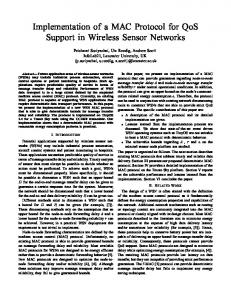
General introduction Approximately every five or ten years we are blessed with the implementation of a new technology that can have a major bearing upon how we live and work. Figure 1 presents a non-exhaustive list of the most implemented cellular telecommunications systems. The development of cellular networks can be classified in different classes (grouped together by technology), each class is known as a generation:

1G  

2G  

3G  

tel-00538837, version 1 - 23 Nov 2010

2.5G   2.75G  

•   AMPS   •   TACS   •   NMT   •   …  

•   GSM   •   CDMA-­‐one   •   PDC   •   PHS   •   …  

•   UMTS   •   CDMA2000   •   …  

•   GPRS   •   EDGE   •   …  

4G  

3.5G   3.75G   •   HSPA   •   EV-­‐DO  /  DV   •   WiMAX   •   …  

•   LTE   •   WiMAX   •   Femto-­‐cell     •   Fexible  radio   •   ?   All-­‐IP  core  

Orthogonal  codes  multiplexing  

Time  and  frequency  multiplexing  

Frequency  multiplexing/FDD  

1980  

Time  

1990  

2000  

2010  

Figure 1: Evolution of Telecommunication systems and rise of network heterogeneity.

1G : Voice communication through analog FM transmission. Frequency Division Multiple Access/Frequency Division Duplexing (FDMA/FDD) was used to accommodate multiple users and channels (1980’s). Advanced Mobile Phone System (AMPS), Total Access Communication System (TACS) and Nordic Mobile Telephony (NMT) were the most used 1G networks. 2G : Were purely digital networks using digital modulation and Time Division Multiple Access (TDMA) or Code Division Multiple Access (CDMA). This generation supports voice, text messaging (SMS) and circuit-switched data communication (1990’s). The two most implemented examples of 2G networks are Global System for Mobile communication (GSM) and Interim Standard 95 (IS-95). Forward error correction (FEC) and encryption are also supported by this generation. Some additional standards were developed to increase the data speeds of 2G networks, including 2.5G General Packet Radio Service (GPRS) and 2.75G Enhanced Data Rates for GSM Evolution (EDGE). 3G : Provides data rates up to 2 Mbps using wideband modulation techniques with increased user capacity (2000’s). Services like Internet, e-mail, multimedia stream27

ing, video telephony and instant messaging are all services available to 3G devices (this includes mobile handsets and computers). The two main 3G standards are Wideband Code Division Multiple Access (WCDMA) and Multi Carrier CDMA (MC-CDMA). Improvements on the 3G standard include 3.5G High Speed Downlink Packet Access (HSDPA) and 3.75G High Speed Uplink Packet Access (HSUPA).

tel-00538837, version 1 - 23 Nov 2010

4G : Higher data rates (up to 1 Gbps) will be supported through the use of an all-IP futuristic network (2010). The multiple access technology used by this generation will be OFDM (Orthogonal Frequency Division Multiplexing), e.g., LTE and WiMAX. The application layer services like mobile video will be provided. There will be seamless integration between all generation networks, which gives rise to interoperable heterogeneous wireless networking. 5G : A recent discussion and research trend on this topic, let imagine a software highly improvement of 4G networks. This generation will mainly base on how a resource should be used and in particular take benefit from the newly concept of virtual Multiple In Multiple Out (MIMO). The idea here is to consider all devices around as virtual antennas in order to improve the instantaneous throughput. Flexible radio called also Software Defined Networks is the most known 5G candidate. The aim behind this successive generations is to facilitate our productivity, and even enhances our recreational capability. In the past we witnessed the PC revolution, the advent of the PDA, and the growth in the use of wireless LANs. Moreover, with the rapid growth in the number of wireless applications, services and devices, using a single wireless technology such as a second generation (2G) and third generation (3G) wireless system would not be efficient to deliver high speed data rate and Quality-ofService (QoS) support to mobile users in a seamless way, see [75]. The next generation wireless systems (also sometimes referred to as Fourth generation (4G) systems) are being devised with the vision of heterogeneity in which a mobile user/device will be able to connect to multiple wireless networks (e.g., WLAN, cellular, WMAN, Mesh) simultaneously. For example, IP-based wireless broadband technology such as IEEE 802.16/WiMAX (i.e., 802.16a, 802.16d, 802.16e, 802.16g) and 802.20/MobileFi will be integrated with 3G mobile networks, 802.11-based WLANs, 802.15-based WPANs, and wireline networks to provide seamless broadband connectivity to mobile users in a transparent fashion. Rather than being an inconvenience, these new heterogeneous networks must indeed be regarded as a new challenge/solution to offer to the users an efficient and ubiquitous radio access, by means of a coordinate use of the available Radio Access Technologies (RATs). In this way, not only the user can be served through the RAT that fits better to the terminal capabilities and service requirements, leading to the “connected everywhere, anytime, anyhow” experience, but also a more efficient use of the available radio resources can be achieved from the operator’s point of view. Now, the heterogeneous network becomes transparent to the final user and the so-called Always Best Connected (ABC) paradigm [56, 75, 116], which claims for the connection to the 28

tel-00538837, version 1 - 23 Nov 2010

RAT that offers the most efficient radio access at each instant, can be achieved. Heterogeneous wireless systems will achieve efficient wireless resource utilization, seamless handoff, global mobility with QoS support through load balancing and tight integration with services and applications in the higher layers. After all, in such a heterogeneous wireless access network, a mobile user should be able to connect to the Internet in a seamless manner. The wireless resources need to be managed efficiently from the service providers point of view for maximum capacity and improved return on investment. The convergence of the different wireless technologies is a contiguous process. With each passing day, the maturity level of the mobile user and the complexity level of the cellular network reach a new limit. Current networks are no longer “traditional” GSM networks, but a complex mixture of 2G, 2.5G, and 3G technologies. Furthermore, new technologies beyond 3G (e.g., HSPA, WiMAX, LTE) are being utilized in these cellular networks. Existence of all these technologies in one cellular network has brought the work of design and optimization of the networks to be viewed from a different perspective. We no longer need to plan GSM, GPRS, or WCDMA networks individually. The cellular network business is actually about dimensioning for new and advanced technologies, planning and optimizing 4G networks, while upgrading 3G/3.5G networks.

Figure 2: Illustrative example of a heterogeneous Wireless Mesh Network.

Protocol engineering and architecture design for broadband heterogeneous wireless access systems is an emerging research area. Load balancing and network selection, resource allocation and admission control, fast and efficient vertical handoff mechanisms, and provisioning of QoS on an end-to-end basis are some of the major research issues related to the development of heterogeneous wireless access networks. This thesis covers different aspects of analysis, design, deployment, and optimization of protocols and architectures for heterogeneous wireless access networks. In particular, the topics include challenges and issues in distributed algorithms design and provision29

tel-00538837, version 1 - 23 Nov 2010

ing of a QoS framework for heterogeneous wireless access networks, architectures and protocols for optimal spectrum utilization in multihop ad hoc wireless networks, network selection in heterogeneous wireless access networks, modeling and performance analysis of heterogeneous mobile networks, quality-oriented multimedia streaming in heterogeneous/multihop ad hoc wireless networks, and extensive simulations.

30

tel-00538837, version 1 - 23 Nov 2010

Motivation and general overview In the near future, multitude of wireless communication network based on a variety of radio access technologies and standards will emerge and coexist. The availability of multiple access alternatives offers the capability of increasing the overall transmission capacity, providing better service quality, dealing with health problems of wireless systems and reducing the deployment costs for wireless access. This way, practically all existing technologies will become simple RATs (e.g., GSM, UMTS, CDMA2000, HSPA, WLANs, WiMAX, LTE, etc.) to access the real network which is henceforth mandatory heterogeneous. In order to exploit this potential multiaccess gain, it is required that different RATs are managed in a cooperative fashion. In the design of such a cooperative network, the main challenge will be bridging between different networks technologies and hiding the network complexity and difference from both application developers and subscribers and provide the user seamless and QoS guaranteed services. The trend will also bring about a revolution in almost all fields of wireless communications, such as network architecture, protocol model, radio resource management, and user terminal as well. As wireless networks grew larger, it became evident that centralized control would be impractical for coordinating all elements of the network, and in particular end-user transmissions. The celebrated Aloha protocol was designed at the early 70’s [2] as a distributed mechanism which can allow efficient media sharing. This protocol and its variants, such as slotted aloha [125] CSMA-CD and tree-algorithms [25], are cooperative in the sense that each user is committed to perform his part of the protocol.

Clearly, modern wireless network protocols are often based on Aloha-related concepts (for example, the 802.11 and 802.16 standards [36, 146, 147, 148]). The design of such protocols raises novel challenges and difficulties, as the wireless arena becomes more involved. The most studied issue is the under-utilization of aloha medium access method (18% using pure aloha and 37% using slotted aloha). The basic underlying assumption in legacy slotted aloha protocols is that any concurrent transmission of two or more users causes all transmitted packets to be lost [10, 13, 25, 125]. However, this model does not reflect the actual situation in many practical wireless networks where some information can be received correctly from a simultaneous transmission of several packets. Therefore, this assumption has been subjected to some improvements in literature. The first improvement is called the capture effect: The packet with the strongest power level can be received successfully (captured) in the presence of contending transmissions if its power level is sufficiently high. It occurs in networks with single packet reception capability where packets arrive at the common receiver with different power levels due to near-far effect, shadowing or fading. The effect of capture on Aloha [3, 18, 87, 89, 112, 132, 136, 169, 170] and on IEEE 802.11 protocol (Carrier Sense Multiple Access-Collision Avoidance (CSMA/CA)) [69, 100, 114] has been studied extensively in the literature and new MAC protocols for channels with capture have been proposed [37]. Despite of the bounty of works and efforts investigated in analyzing aloha-like protocols with capture effect our approach is different. We propose to consider a random choice of a power level and fine-tune the transmit probability in or31

tel-00538837, version 1 - 23 Nov 2010

der to maximize the objective function. Through the first part of this thesis we define a stochastic game where mobiles are assumed to be selfish and develop many distributed schemes with several power level setups. Moreover, the researchers community usually focuses on saturated users, i.e., users have all the time packets to be transmitted. Here, we analyze the non saturated case with an infinite buffer capacity. In contrast to saturated users with a fixed throughput demand, two equilibria may exist [104]. This issue is then to be addressed when relaxing the saturation assumption. Hajek et al. [70] provided asymptotic results on the capture probability in the limit of infinite number of users, see also [34] and references therein for detailed overview. The other major improvement to the original protocol, known as multipacket reception capability, assumes that a subset of the collided packets can be received successfully. The impact of the multipacket reception capability on MAC protocols has received limited attention to date. Ghez et al. [63, 64] proposed a channel model for networks with multipacket reception capability and studied stability properties of slotted aloha in such a setting. Tong et al. have proposed MAC protocols based on multipacket reception capability [106, 107, 167, 168] using the channel model suggested in [63]. The protocols developed in [167, 168] maximize the normalized throughput by controlling the set of users who are allowed to transmit in each slot. However, these protocols require a centralized controller and hence are impractical for large distributed networks. [122] presents a pseudo PHY/MAC cross-layered approach for multipacket reception. Despite its advantages, the cellular concept (or infrastructure-based wireless networks, to be more general), has its drawbacks: it is of relatively low bandwidth, similar in many ways to wired dial-up access, and it generally takes time and potentially high cost to set up the necessary infrastructure [65]. Moreover, even if costs were reduced and efficiency improved, infrastructure-based networks may not always be possible, scalable, appropriate, or even desirable in many of the envisaged scenarios for ubiquitous and pervasive computing/communications. To fulfill the vision of ubiquitous computing/communications, wireless networks need to evolve beyond the current infrastructure-type of networks. Fortunately, because of significant advances in hardware technology in the past decades - most notably in the areas of processing capability and storage capacity- it has now been possible to include more “intelligence” into smaller devices with significant reductions in power consumption and higher performances. As a consequence, the deployment of wireless networks without any preexistent infrastructure ( the so-called wireless ad hoc networks) are now becoming possible. Although derived from military research into mobile networks1 , the emergence of multihop ad hoc and Mobile ad hoc networking (MANET, [66, 67]) has its greatest potential in the commercial marketplace and is the one of key points of this dissertation. Each node operates not only as a host but also as a router, forwarding packets on behalf of other nodes that may not be within direct wireless transmission range of their desti1

Initial interest in ad hoc networks emerged within the military arena with the Packet Radio Network project funded by the Defense Advanced Research Projects Agency in 1972, followed by the Survivable Radio Networks project in 1983, and DARPA’s Global Mobile Information Systems program in 1994 [58].

32

tel-00538837, version 1 - 23 Nov 2010

nations. In recent years, the research in ad hoc networks becomes more and more dedicated to specialized network applications like Wireless Mesh Networks (WMN) [5, 76], opportunistic networks, Wireless Sensor Networks (WSN) and vehicular ad hoc networks (VANET). This kind of ubiquitous networks are dynamically self-organized and self-configured, with the nodes in the network automatically establishing and maintaining mesh connectivity among themselves (creating, in effect, an ad hoc network). This feature brings many advantages such as low up-front costs, easy network maintenance, robustness, and reliable service coverage. However, the main contribution of “general” ad hoc networks research consists on the understanding of the constraints and limitations of such wireless networks [39, 50]. The multi-hop nature of such networks and the broadcast nature of wireless channel are responsible of many challenges and hard issues. Since the current design of ad hoc networks is based on the standard OSI layered approach, significant research was occupied to propose new protocols at different layers independently to combat the network limitations. Despite the flexibility and the simplicity of layered model, it leads to poor performance and thus a cross-layer protocol design is needed. In a cross-layer design an information in a given layer is made available to protocols in different layers which enable resource optimization and therefore promises more efficient performance improvement. Moreover, carrier sensing is widely adopted in wireless communication to protect data transfers from possible collisions. e.g., distributed coordination function (DCF) in IEEE 802.11 standard renders a node to defer its communication if it senses the medium busy. However, even if the carrier signal is detected to be greater than the threshold, both ongoing and a new communication can be simultaneously successful depending on their relative positions in the network or equivalently, their mutual interference level. Therefore, supporting multiple concurrent communications is important in multihop ad hoc networks in order to maximize the network performance and improve the reuse factor of the common channel. However, it is largely ignored in DCF of the 802.11 standards because it is primarily targeted at single-hop wireless LANs [144]. This latter point justifies the need to adapt/design dedicated protocols for multihop communications instead of reusing infrastructure-based standards. In [21], the authors achieved a high throughput and low delay in ad hoc networks. El Gamal et al. [59] analyzed the optimal delay-throughput scaling for different wireless network topologies. In the static random network with n nodes, they obtained an optimal tradeoff between throughput and delay. A plenty of other trials concerning the stability, capacity and delay in ad hoc networks were performed, see e.g. [62, 91, 108, 162].

33

tel-00538837, version 1 - 23 Nov 2010

Our contributions This dissertation focuses on the developing new version of slotted aloha like random access protocols and ad hoc networks performance using multi-layer parameters and forwarding capability. The performance metrics of interest are throughput, delay, stability of forwarding queues and energy consumption. The chapters are organized in three parts. The first part deals with the under utilization problem of wireless collision channels. In the second part, we based our study on performance evaluation of a WiMAX/ad hoc integrated network. We developed an analytical model using a new cross-layer approach with a weighted fair queueing scheduler. We are then able to differentiate between packets to be forwarded and new entering packets. Tracking traffic is now easy and very comprehensive. The last part is dedicated to extending the previous model to IEEE 802.11e DCF/EDCF. We indeed integrate APPLICATION, NETWORK, MAC and PHY layers in a unified cross-layered model. This way, the modeling framework focuses on the interactions between several layers, and on the impact that each node has on the dynamics of every other node in the network. A key feature of our model is that nodes can be modeled individually, i.e., it allows a per-node setup of many layer-specific parameters. Moreover, no spatial probability distribution or special arrangement of nodes is assumed; the model allows the computation of individual (per-node/per-path) performance metrics for any given network topology and radio channel model. This later feature gives very important insight to judiciously set each parameter taking into account the information coming from other layers. Our main contributions and the outline of the chapters content are the following Chapter 1 : Slotted Aloha with Random Power Level Selection and Capture Effect. We consider the uplink case of a cellular system where m bufferless mobiles transmit over a common channel to a base station, using the slotted aloha medium access protocol. The novelty here is the consideration of several power differentiation schemes. Indeed, we consider a random set of selectable transmission powers and further study the impact of priorities given either to new arrival packets or to the backlogged ones. Later, we address a general capture model where a mobile transmits successfully a packet if its instantaneous SINR (signal to interferences plus noise ratio) is lager than some fixed threshold. Under this capture model, we analyze both the cooperative team in which a common goal is jointly optimized as well as the noncooperative game problem where mobiles seek to optimize their own objectives. Furthermore, we derive the throughput and the expected delay and use them as the objectives to optimize and provide a stability analysis as an alternative study. Exhaustive performance evaluations are performed, we showed that schemes with power differentiation improve significantly the individual and the global performances.They also could eliminate in some cases the bi-stable nature of slotted aloha. Chapter 2 : Sustaining Partial Cooperation in Hierarchical Wireless Collision Channels. In a spirit similar to that of Chapter 1, we consider a wireless system composed of one central receiver and several selfish transmitters communicating via the 34

tel-00538837, version 1 - 23 Nov 2010

slotted aloha protocol. The set of users is split into two classes: Leaders and Followers. Then, we study the induced non-cooperative hierarchical game based on the Stackelberg equilibrium concept. Each user seeks to maximize his own throughput or to minimize the expected delay experienced by its backlogged packets. Those utility functions are clearly depending on the individual transmission probability and the transmission probabilities of all other concurrent users in the network. Using a 4D Markovian model, we compute the steady state of the system and derive the average throughput and the expected delay as well. We start by discussing the protocol design and propose a controlled slotted aloha using a virtual controller that make the channel lossy to reduce the channel access of concurrent users. Later, we investigate the impact of introducing hierarchy in such a random access protocol and discuss how to distribute leader/follower roles. Furthermore, exhaustive performance evaluations are carried out, we show that the global performance of the system is improved compared to standard slotted aloha system. However, a slight performances slow-down may be observed for the followers group small number of users.

Chapter 3 : Learning Constrained Nash Equilibrium in Wireless Collision Channels. We consider a finite number of users, with infinite buffer storage, sharing a single channel using the aloha medium access protocol. This is an interesting example of a non saturated collision channel. We investigate the uplink case of a cellular system where each user will select a desired throughput. The users then participate in a non cooperative game wherein they adjust their transmit rate to attain their desired throughput. We show that this game, in contrast to the saturated case where two equilibria may exist, either has no Nash Equilibrium or has infinitely many Nash Equilibria. Further, we show that the region of NE coincides with an appropriate ’stability region’. We also discuss the efficiency of the equilibria in term of energy consumption and congestion rate. Next, we propose two learning algorithms using a stochastic iterative procedure that converges to the best Nash equilibrium. For instance, the first one needs partial information (transmit rates of other users during the last slot) which can be estimated by observing enough the system behavior. The second is an information-less and fully distributed scheme. We approximate the control iterations by an equivalent ordinary differential equation in order to prove that the proposed stochastic learning algorithm converges to the desired Nash equilibrium even in the absence of any coordination or extra information. Extensive numerical examples and simulations are provided to validate our results.

Chapter 4 : Performance Evaluation of WiMAX and Ad hoc Integrated Networks. Current mobile users are often equipped with several network interfaces, which may be of different access technologies. Each access technology has specific characteristics in terms of coverage area and technical characteristics (bandwidth, QoS, etc.) and provides diverse commercial opportunities for the operators. It seems likely that these various technologies have to coexist and, from then, solutions of integration and interoperability will be necessary to deal with the technological diversity. We consider in this chapter the WiMAX and ad hoc integrated networks. A user who needs to estab35

tel-00538837, version 1 - 23 Nov 2010

lish a high reliable service prefers to use WiMAX network and another who needs to transmit Best Effort traffic with high rate but delay tolerant prefers to connect ad-hoc network that is assumed to have access to Internet. We aim through this combination to locally extend the coverage of the WiMAX cell and to study the stability of involved nodes, in particular, gateway nodes. Under stability condition, our main result is characterization of the end-to-end throughput and delay using the rate balance equation and a G/G/1 queueing model. Through numerical results, we demonstrate the utility and efficiency of our approach.

Chapter 5 : Asymptotic Delay in Wireless Ad hoc Networks with Asymmetric Users. In this chapter, we present an analytical model for an approximate calculation of the end-to-end delay performance in multihop wireless ad hoc networks. In contrast to literature that largely focuses on average delay, our work focuses on the distribution of end-to-end delay. Now, we assume that each source injects packets in the network, which traverse intermediate relay nodes until they reach the final destination. Firstly, we employ discrete-time queueing theory to derive the expressions for the queue length and the delay in terms of probability generating functions. Secondly, in order to improve the control routing and transmission scheduling, we adopt a new architecture that allows information sharing across different layers for efficient utilization of network resources, and meeting the end-to-end performance requirements of demanding applications. Thirdly, we propose a cross-layered packet admission control scheme based on delay timeout mechanism. This guarantees quality of service for multimedia applications such as voice and video streaming. Finally, we conduct extensive simulations in order to verify and assist our analytical results.

Chapter 6 : A Cross-layered Modeling of IEEE 802.11-Operated Ad hoc Networks. Performance of IEEE 802.11 in multi-hop wireless networks depends on the characteristics of the protocol itself, and on those of the upper layer routing protocol. We are interested here in modeling the IEEE 802.11e enhanced distributed coordination function (EDCF) networks. We investigate the intricate interactions between several PHY, MAC and Network layer parameters, including the carrier sense threshold, the contention window size, limit number of retransmissions, multi rates, routing protocols and the network topology. In fact, we are focusing to study the effect of cooperation and PHY/MAC parameters on the stability and the throughput of ad hoc networks. We extend the results of [166] to a multi-hop ad hoc network with asymmetric topology and asymmetric traffic loads using a cross-layer architecture. We develop an analytical model that predicts the throughput of each connection as well as the stability of forwarding queues of intermediate nodes. Performance of such a system is also evaluated via simulations. To the best of our knowledge, our work is the first to consider asymmetric topology of the network and asymmetric parameters in PHY/MAC layers. We show that the performance measures of MAC layer are affected by the intensity of traffic of a connection that an intermediate node forwards. More precisely, the attempt rate and the collision probability are now dependent on the traffic flows, topology and routing. 36

tel-00538837, version 1 - 23 Nov 2010

Chapter 7 : Fountain Code-based Fair IEEE 802.11-Operated Ad hoc Networks. Our objective in this chapter is to study a class of transmission mechanisms that include coding in order to improve the probability of successful delivery within a multihop ad hoc network. We propose an analytical approach that allows to quantify tradeoffs between throughput and fairness. We study the effect of coding on the performance of the network while optimizing parameters that govern NETWORK, MAC and PHY layers. In other words, this chapter extends the multi-layered model discussed in the previous chapter. We present a solution based on coding packets at MAC layer before transmitting them over the common channel. To the best of our knowledge, we are the first to use Fountain codes at MAC layer level. Indeed, coding packets is usually studied at APPLICATION [51, 53, 95, 140] or TRANSPORT layers, see e.g., [86]. In standard IEEE 802.11, whenever a collision occurs the whole packet is lost and needs to be retransmitted after the random backlog period. Our solution uses an incremental combination of all previous copies of a backlogged packet to improve the decoding probability and therefore to correctly recover the original packet. As we expected, using Fountain code in our context increase the Jain’s Fairness index over the network. It indeed improves the throughput on paths that suffer from high collision probability. However unfortunately, it may decrease the throughput on the other paths. This is due to the injected redundancy in coded packets and its negative effect that reduces the channel idle period seen by concurrent users.

37

38

tel-00538837, version 1 - 23 Nov 2010

tel-00538837, version 1 - 23 Nov 2010

Part I

On Improving Wireless Collision Channels Utilization

39

tel-00538837, version 1 - 23 Nov 2010

Chapter 1

tel-00538837, version 1 - 23 Nov 2010

Slotted Aloha with Random Power Level Selection and Capture Effect Contents

1.1

1.1

Introduction . . . . . . . . . . . . . . . . . . . . . . . . . . . . . . . . . .

41

1.2

Problem formulation . . . . . . . . . . . . . . . . . . . . . . . . . . . . .

44

1.3

The Team Problem . . . . . . . . . . . . . . . . . . . . . . . . . . . . . .

46

1.4

Game problem . . . . . . . . . . . . . . . . . . . . . . . . . . . . . . . .

56

1.5

Numerical investigation . . . . . . . . . . . . . . . . . . . . . . . . . . .

59

1.6

Concluding remarks . . . . . . . . . . . . . . . . . . . . . . . . . . . . .

70

Introduction

Aloha [2] and slotted aloha [125] have long been used as randomly distributed medium access protocols for radio channels. They are used in satellite networks and cellular telephone networks for the sporadic transfer of data packets. In these protocols, packets are transmitted sporadically by various users. If packets are sent simultaneously by more than one user then they collide. After a packet is transmitted, the transmitter receives the information on whether there has been a collision (and retransmission is needed) or whether it has been well received. All colliding packets are assumed to be corrupted which get backlogged and are retransmitted after some random time. We focus on the slotted aloha [25], in which time is divided into units. At each time unit a packet may be transmitted, and at the end of the time interval, the sources get the feedback on whether there was zero, one or more transmissions (collision) during the time slot. A packet that arrives at a source is immediately transmitted. Packets that are involved in a collision are backlogged and are scheduled for retransmission after a random time.

41

tel-00538837, version 1 - 23 Nov 2010

Chapter 1. Slotted Aloha with Random Power Level Selection and Capture Effect

Interest has been growing in recent years in studying competition of networking in general, access to a common medium in particular, within the frame of non-cooperative game theory, see e.g. the survey paper [11]. Various game formulations of the standard Slotted Aloha (with a single power) have been derived and studied in [12, 9, 8, 81, 98, 99] for the non-cooperative choice of transmission probabilities. In [9, 12, 13, 44], authors consider slotted Aloha system as both cooperative (where a common objective is jointly optimized) and non cooperative game, where each users fine-tunes its transmit probability to maximize its payoff, with partial information and power diversity. In [81], the authors discuss the equilibrium of a non-cooperative game for Aloha protocols. In their game formulation, Users are heterogeneous and each one fine-tunes its transmit probability in order to guarantee its demand. Mackenzie et al. [99] discusse the stability of slotted Aloha with selfish users behavior and perfect information. The authors showed the existence of an equilibrium and characterized it. In [110] it is shown that the system capacity could be increased from 0.37 to 0.53 if one class of terminals always uses high power and the other always uses low power level. In [87], power diversity is studied with the capture model that we use as well as with another capture model based on signal to noise ratio. [133] studies power diversity under three types of power distribution between the power levels and provides also a detailed stability analysis. [96] proposes a model and evaluates the throughput that can be achieved in a system of N mobiles using generalized aloha like protocols where the mobiles transmit data using a two-state decision system. For cooperative systems, it gives the throughput bounds and explores the tradeoff between throughput and short-term fairness. But our proposal is different here, we address the effect of randomization in power levels for both cooperative and non-cooperative setups. When multiple users share a common channel and contend for access, a typical conflict problem arises. Recently, the selfish behavior of users in MAC protocols has been widely analyzed using game theory with all its powerful solution concepts. It was shown in [8, 13, 44] and [115] that the users selfish behavior likely leads to a network collapse, where a typical prisoners dilemma situation occurs. This illustrates, in fact, that Nash equilibrium1 (NE) is not efficient in some situations. This way, full system utilization requires coordination among users using explicit message exchanges or presence of an arbitration mechanism [10], which may be impractical given the distributed nature and arbitrary topology change (due to mobility, ended calls, new calls, environment, ...) of wireless networks. To achieve a better performance without coordination schemes, users need to sustain cooperation or priority. It is beneficial to design a set of users whose mission is to provide incentives for other users to behave cooperatively as well as respect the defined priority, this mechanism may limit the aggressiveness level (access to the channel) and resolve the contention/random problem. Another way to reduce the access contention is to introduce a transmission cost. Indeed, it was shown in [101] that costs have a stabilizing effect; being rational, users will defer packet transmissions when congestion develops and the cost for successful 1

A Nash equilibrium of a game is a strategy profile such that no player can improve its reward by changing its strategy, assuming the complementary strategies of the other players stay the same. The strategies here are said to be “mutual best responses”.

42

tel-00538837, version 1 - 23 Nov 2010

1.1. Introduction

transmission becomes high. This way, users will drop packets when the total transmission costs are high which can cause a huge delay and then the analysis seems to be not applicable to delay-sensitive traffic. Authors in [128], showed that introducing users hierarchy improve the performances of the whole system and the enhancement depends on the offered load. At low load, this improvement is due to the fact that users (both of leaders and followers) retransmit with high probability at low load, hence the backoff time is reduced. At average and high loads, leaders turn to be generally less aggressive than Nash equilibrium case. This way, the collision probability is reduced and then the performance of the hierarchical scheme are enhanced. A pretty phenomena, when the number of followers becomes larger than the number of leaders, is that those latter users become more friendly and reduce their retransmission probability, whereas the followers become very aggressive and transmit at probability close to 1. Here, we extend the model first proposed in [8] and introduce new schemes in which multiple power levels are used for transmission. When several packets are sent simultaneously, one of them can often be successfully received due to the power capture effect. In this chapter, we consider a general capture model where a mobile transmits successfully a packet if his instantaneous SINR (signal to interferences plus noise ratio) is lager than the fixed threshold. In particular, we introduce the differentiation between new packets and backlogged packets allowing prioritization of one or the other in terms of transmit power. We study and compare the following schemes: 1. The first scheme considers the power diversity but defines no prioritization in transmission or retransmission. This scheme will mainly show the effect of power diversity on system performances; 2. In the second scheme, each new packet is immediately transmitted with the lowest power, whereas backlogged packets are sporadically retransmitted at a random power selected among N − 1 larger distinct levels; 3. Here, new packets are transmitted with the highest power, and backlogged packets are retransmitted at a random power level picked from N − 1 lower distinct levels; 4. This scheme Gives more priority to new arrivals. Indeed,backlogged packets are retransmitted with the lowest power level and a new packet is transmitted at a random power selected among N − 1 larger distinct levels. 5. All previous schemes are compared with standard slotted aloha taken as reference, this allows to compare and analyze performances of each scheme. The capture model used in [8] is not realistic, authors assume therein that when a unique mobile chooses the highest power, compared to other mobiles, its transmission is succeeded independently of the other mobiles and their respective choices. This assumption could not be always true. Indeed, the aggregate signal of other mobiles may jam the signal of the tagged mobile, i.e., whose power level is the highest, therefore no successful transmission exists. Now, a terminal succeeds its transmission if it chooses the most elevated power level compared to other mobiles and its instantaneous SINR 43

tel-00538837, version 1 - 23 Nov 2010

Chapter 1. Slotted Aloha with Random Power Level Selection and Capture Effect

is greater than a given threshold γth . Under more general capture model, we study the team problem in which we optimize transmission probabilities for the various schemes so as to achieve the maximum throughput or to minimize the expected delay. We discover however that in heavy load, the optimality is obtained at the expense of huge expected delay of backlogged packets (EDBP). We therefore consider the alternative objective of minimizing the EDBP. We study both the throughput as well as the delay performance of the global optimal policy. We also solve the multi-criteria problem in which the objective is a convex combination of the throughput and the EDBP. This allows in particular, to compute the transmission probabilities that maximize the throughput under a constraint on EDBP, which could be quite useful for delay-sensitive applications (e.g., Video streaming, Voice, VoD, ...). We show that schemes with priority do not only improve the average performances considerably but they are also able in some cases to eliminate the bi-stable nature of the slotted aloha. Furthermore, we study the game problem in which each mobile chooses its transmission probability selfishly in order to optimize its own objective. This gives rise to a game theoretic model in which we study the equilibrium properties (Nash equilibrium). We show that the power diversity and the prioritization profit to mobiles also in this competitive scenario even if the advantage is less notorious than in the team’s behavior.

1.2

Problem formulation

We consider a collision channel used by one central receiver and m mobiles without buffer, i.e., mobiles do not generate new packet till the current one is successfully transmitted. This assumption can have realistic application in the context of signaling. Indeed, it is natural to assume that a source does not start generating a new signaling packet (e.g., a new reservation) as long as the current signaling packet is not transmitted successfully. Here, the process of attempts to retransmit a new packet from a source after the previous packet has been successfully transmitted corresponds well with our bufferless model. At the beginning of any slot, each mobile can transmit a packet using a power level among N available levels P = { p1 , p2 , ..., p N }. We consider a general capture model where a packet transmitted by a mobile i is received successfully when and only when its instantaneous SINR is larger than some given threshold γth . Let pi be the transmit power chosen by mobile i in the current slot, and σ2 be the spectral density of the background noise which is assumed to be AWGN and time-independent. Let us denote by gi the gain experienced by mobile i over the channel. It depends on the distance between the mobile and the AP, but it is also impacted by the reflective paths. The instantaneous SINR of mobile i received by the central receiver is given by γi =

gi p i k

∑ g j p j I ( j) + σ

j =1

44

, 2

(1.1)

1.2. Problem formulation

tel-00538837, version 1 - 23 Nov 2010

where I ( j) is indicator of the event that at the current slot, user j is transmitting. We address here a random power selection fashion where transmit powers are selected according to a probability distribution X = [ x1 , x2 , ..., x N ], i.e., power level p j is chosen with probability x j . The impact of selection probability distribution will be discussed in Subsection 1.5. In particular, we propose to discuss the case of 1) uniform distribution; 2) high power levels are prioritized and; 3) the case where low power levels are prioritized. We extend here the Markovian model first described by Altman et al. [8, 9, 13] in order to incorporate the instantaneous capture effect. The arrival probability of the packets to the source i follows a Bernoulli process with parameter q a (i.e., at each time slot, there is a probability q a of a new arrival at a source, and all arrivals are independent). As long as there is a packet at a source (i.e., as long as it is not successfully transmitted) new packets to that source are blocked and lost (because we consider sources without buffer). The arrival processes of different sources are assumed to be independent. Similarly, we consider that a backlogged packet at source i is retransmitted with probability qri . We should restrict in our control and game problems to simple policies in which qri does not change in time. We also will be interested in the case of symmetric sources, we should then find a symmetric optimal solution, i.e., a retransmission probability qr which does not depend on i. Next, we consider as a state of the system the stochastic process representing the number of backlogged packets in the beginning of a slot, we denote it n. For any choice of values qri ∈ (0, 1] , the state process is a Markov chain that contains a single ergodic chain (and possibly transient states as well). Define q¯ r to be j the vector of retransmission probabilities for all users (whose jth entry is qr ). We note the transition matrix of the Markov chain by P(q¯ r ). Let π¯ (q¯ r ) be the corresponding vector of the steady-state probabilities where its nth entry πn (q¯ r ) denotes the probability of n backlogged mobiles. When all entries of q¯ r are the same, say q, we shall write (with some abuse of notation) π¯ (q) instead of π¯ (q¯ r ). We introduce further notation, assume that there are n backlogged packets, and all use the same value qr for retransmission rate. We denote by Qr (i, n) the probability that i mobiles out of the n backlogged packets retransmit at the current slot. Then   n Qr (i, n) = (1 − qr ) n −i ( qr ) i . (1.2) i Let Q a (i, n) be the probability that i unbacklogged mobiles transmit packets in a given slot (i.e., that i arrivals occurred at mobiles without backlogged packets). We have   m−n Q a (i, n) = (1 − q a ) m − n −i ( q a ) i . (1.3) i Let Qr (i, 0) = 0 and Q a (i, m) = 0. For ease of reading, we summarize the assumptions of our contention model as follows 45

Chapter 1. Slotted Aloha with Random Power Level Selection and Capture Effect

• A finite set of m bufferless mobiles interacts over a single collision channel. • Time is divided into multiple equal and synchronized slots. Transmission feedback (success or collision) are received in the end of the current slot. • Each user i is assumed to be non saturated, packets arrive from higher layers according to a Bernoulli process with parameter q a . • Each user i retransmits, in every slot, its packets with probability qri .

tel-00538837, version 1 - 23 Nov 2010

• The average throughput or minus expected delay of backlogged packets are the objective functions to maximize. Remark 1.2.1. Quite frequently one uses the ALOHA protocol for sporadic transmissions of signaling packets such as packets for making reservation for a dedicated channel for other transmissions (that do not use ALOHA), see e.g. the description of the SPADE on demand transmission protocol for satellite communications in [135]. In the context of signaling, it is natural to assume that a source does not start generating a new signaling packet (e.g. a new reservation) as long as the current signaling packet is not transmitted. In that case, the process of attempts to retransmit a new packet from a source after the previous packet has been successfully transmitted coincides with our no buffer model.

1.3

The Team Problem P(n-1,n+2) P(n-1,n+1)

¬

P(n,n+1)

P(n-1,n) n-1

n

P(n+1,n+2) n+1

P(n,n)

n+2

¬

P(n+2,n+1)

P(n+1,n)

P(n,n-1) P(n-1,n-1)

P(n,n+2)

P(n+1,n+1)

P(n+2,n+2)

Figure 1.1: Markov chain for the team problem. The state of the system is the backlog, it can decrease by at most one per transition but can increase by an arbitrary amount less than or equal m − n.

We first study slotted aloha in a team problem point of view, i.e., all mobiles optimize the same objective function (maximize the system throughput or minimize the average delay). Here, we analyze the case when there exists a central entity (base station, dedicated device, ...) that computes the optimal strategy profile and broadcasts it to operating mobiles. This entity should know the total number of mobiles and their individual new arrivals intensity q a . Next, we allow prioritization by incorporating a selective transmit power allocation mechanism. On the beginning of each slot, each mobile picks a power level from the N available power levels and decides to transmit/retransmit its packet. The corresponding Markov chain is depicted in figure 1.1. Based on power allocation fashion, we analyze the following four schemes. 46

1.3. The Team Problem

1.3.1

Scheme 1 : Random power levels without priority

tel-00538837, version 1 - 23 Nov 2010

We assume that there is no preference between new packets or backlogged ones. A mobile chooses to transmit using randomly a power level among N available levels. In case all mobiles attempt the channel with the same probability q, the transition probabilities of the system are given by

Pn,n+i =

 n   Q ( m − n, n ) a  ∑ Qr ( j, n)(1 − A j+m−n ), i = m − n, i ≥ 2   j =0    n     Q a (i, n) ∑ Qr ( j, n)(1 − A j+i )    j =0    n    + Q ( i + 1, n ) Qr ( j, n) A j+i+1 , 2 ≤ i < m−n  a ∑    j =0   n     Q ( 1, n ) Qr ( j, n)(1 − A j+1 ) a  ∑  j =1

n    + Q a (2, n) ∑ Qr ( j, n) A j+2 ,    j =0    n    Q ( 0, n )[ Q ( 0, n ) + Qr ( j, n)(1 − A j )]  a r ∑    j =2   n     + Q ( 1, n ) a  ∑ Qr ( j, n) A j+1 ,    j =0   n      Q a (0, n) ∑ Qr ( j, n) A j ,

i=1

i=0 i = −1

j =1

where Ak is the probability of a successful transmission among k ≥ 2. Denote by aik the event that transmission of some tagged mobile i is successful when having k − 1 other simultaneous transmissions. It can be derived by the following decomposition aik = N

∑ P(mobile i transmits with power level pt

∩ other mobiles transmit with powers less than pt

t =2

∩ SINR of mobile i is greater than the threshold γth ). Sine mobiles are assumed to be symk

metric, then Ak =

∑ aik = k.aik , it follows that

i =1

N −2 k −1 k −1

Ak = k

∑ ∑ ∑

k −1

···

l =0 k 1 =0 k 2 =0

·u

∑

k N − l −1 = 0

p N −l ∑sN=−1l −1 ps k s + σ2 /g

x1k1 ·

k x2k2 · · · x NN−−ll −−11

· x1N −l · δ k − 1 −

!

N − l −1

∑

ks

s =1

!

− γth ,

(1.4)

with A0 = 0 and A1 = 1. xs denotes the probability that a user (with new arrival or backlogged packet) (re)transmits using power level ps . p N −l is the power level chosen by the terminal whose transmission maybe potentially succeed, i.e., it’s corresponding to the highest power selected in the current slot. Whereas k s denotes the number of 47

Chapter 1. Slotted Aloha with Random Power Level Selection and Capture Effect

terminals those choose the power level ps . δ(t) (Dirac distribution) and u(t) (unite echelon) are defined as following



tel-00538837, version 1 - 23 Nov 2010

δ(t) =

1 0

if



t=0 else

u(t) =

1 0

if

t≥0 else

(1.5)

Computing the success probability is a very hard issue. The difficulty in formula (1.4) is to consider one single transmitting mobile at the highest power level and list all the cases where the k − 1 remaining mobiles transmit at lower power. This corresponds exactly to the set of partitions 2 of the positive integer k − 1 considering all possible permutations. Generating all the partitions of an integer is widely studied in the literature and several algorithms were proposed, e.g., see [16] and [124]. The computational complexity of such algorithms is very high and may takes long time to list the set of all partitions as well as their permutations. However, in our model the success probability depends on none of the following: the instantaneous backlog of the system n; the arrival probability q a ; and, the retransmission probability qr . Henceforth, success probability matrix A = ( Ak ), k = 1 · · · m can be calculated once and reused to derive the transition matrix.

1.3.2

Scheme 2 : Retransmission with more power

Now, backlogged packets are assumed to have more priority; a tagged mobile having a backlogged packet retransmits it using a random power level among the N available, while a mobile with a new arrived packet uses always the lowest power level (p1 ). A successful capture is occurred when a backlogged packets is transmitted at a power level larger than those chosen by all other transmitters and the AP experiences an SINR larger than the threshold γth , or a single new arrival occurs and there is no retransmission attempt by any backlogged users. The transition probabilities are then given

2

A partition of a positive integer n is a way of writing n as a sum of positive integers.

48

1.3. The Team Problem

by

tel-00538837, version 1 - 23 Nov 2010

Pn,n+i =

 n   Q ( m − n, n ) Qr ( j, n)(1 − Bj,m−n ), i = m − n, i ≥ 2 a  ∑   j =1    n     Q a (i, n) ∑ Qr ( j, n)(1 − Bj,i )    j =0    n    + Q ( i + 1, n ) Qr ( j, n) Bj,i+1 , 2 ≤ i < m−n  a ∑    j =1   n     Q ( 1, n )  ∑ Qr ( j, n)(1 − Bj,1 )  a j =1

n    + Q ( 2, n ) a ∑ Qr ( j, n) Bj,2 ,    j =1    n    Q ( 0, n )[ Q ( 0, n ) +  a r ∑ Qr ( j, n)(1 − Bj,0 )]    j =2   n     + Q a (1, n) ∑ Qr ( j, n) Bj,1 ,     j =0   n      Q a (0, n) ∑ Qr ( j, n) Bj,0 ,

i=1

i=0 i = −1

j =1

where the probability of a successful transmission among k retransmissions and k0 new arrival packets (k + k0 ≥ 2) is given by

N −2 k −1

Bk,k0

= k

∑ ∑

l =0 k 1 =0

·u

···

k −1

N − l −1

k N − l −1 = 0

i =1

∑

∏

xiki

·

x1N −l

!

N − l −1

·δ k−1−

∑

ks

s =1

!

p N −l ∑sN=−1l −1 ps k s + k0 p1 + σ2 /g

− γth ,

(1.6)

with B0,0 = 0, B0,1 = 1 and B1,0 = 1.

1.3.3

Scheme 3 : Retransmission with less power

New arrivals are now transmitted at the highest power level , i.e., p N , whereas mobiles having backlogged packets attempt new retransmission using a random power picked 49

Chapter 1. Slotted Aloha with Random Power Level Selection and Capture Effect

from N − 1 distinct lower power levels. The transition matrix is summarized as

Pn,n+i =

 Q a (i, n), 2≤i    n    Q a (1, n) ∑ Qr ( j, n)(1 − Cj,1 ), i=1     j = 1   n     Q a (0, n)[ Qr (0, n) + ∑ Qr ( j, n)(1 − Cj,0 )] j =2

 n     + Q ( 1, n ) a ∑ Qr ( j, n)Cj,1 ,    j =0    n    Q ( 0, n )  ∑ Qr ( j, n)Cj,0 ,  a

i=0 i = −1

tel-00538837, version 1 - 23 Nov 2010

j =1

where the probability of a successful transmission when k ≥ 1 mobiles attempt retransmissions is given by the following expression k −1 k −1

Ck,1 = k

∑ ∑

k −1

···

k 1 =0 k 2 =0

·u

N −1

∑ ∏

k N −1 = 0 i = 1

xiki

· x1N −l · δ k −

!

N −1

∑

ks

s =1

pN − γth N −1 ∑s=1 ps k s + σ2 /g

! .

(1.7)

Similarly, the probability of a successful retransmission among k ≥ 2 simultaneous retransmissions is given by N −2 k −1 k −1

Ck,0 = k

∑ ∑ ∑

···

l =1 k 1 =0 k 2 =0

·u

whereas

1.3.4

Ck,k0 = 0

k −1

N − l −1

k N − l −1 = 0

i =1

∑

∑sN=−1l −1 ps k s + σ2 /g K 0 ≥ 2,

·

x1N −l

!

N − l −1

·δ k−1−

∑

ks

s =1

!

p N −l

if

∏

xiki

− γth ,

C0,1 = 1

and

(1.8)

C1,0 = 1.

Scheme 4 : Retransmission with the lowest power

In this last proposal, a new transmitted packet uses a power among N − 1 higher available power levels. Mobiles having backlogged packet retransmit with the lowest power 50

1.3. The Team Problem

level, i.e., p1 . The transition matrix of the Markov chain is given by

tel-00538837, version 1 - 23 Nov 2010

Pn,n+i

 n    Q ( m − n, n ) Qr ( j, n)(1 − D j,m−n ), i = m − n, i ≥ 2 a ∑    j =0    n    Q ( i, n ) Qr ( j, n)(1 − D j,i )  a ∑    j =0   n     + Q ( i + 1, n ) Qr ( j, n) D j,i+1 , 2 ≤ i < m−n  a ∑    j =0   n    Q (1, n) Qr ( j, n)(1 − D j,1 ) a ∑ = j =1   n    + Q a (2, n) ∑ Qr ( j, n) D j,2 , i=1     j =0   n     Q ( 0, n )[ Q ( 0, n ) +  a r ∑ Qr ( j, n)(1 − Dj,0 )]    j =2   n     + Q a (1, n) ∑ Qr ( j, n) D j,1 , i=0    j =0    Q a (0, n) Qr (1, n), i = −1

where Dk,k0 represents the probability of a successful new transmission among k backlogged packets and k0 new packets such that k0 + k ≥ 2. The value Dk,k0 is given by Dk,k0

= k

0

N −2 k −1

∑ ∑

···

l =0 k01 =0

·u

k 0 −1

N − l −1

k0N −l −1 =0

i =1

∑

∏

k0 xi i

·

x1N −l

0

·δ k −1−

N − l −1

∑

p l =1

! k0pl

!

p N −l − l −1 pl k0pl + kP1 + σ2 /g ∑N p l =1

− γth ,

(1.9)

where D0,0 = 0, D0,1 = 1 and D1,0 = 1

1.3.5

Performance metrics

We now turn to present the performance measures (average throughput and expected delay) of interest for optimization as a function of the steady-state probabilities of the Markov chain. Let us denote by πn (q) the equilibrium probability that the network is in state n (number of backlogged packets at the beginning of a slot). Hence the equilibrium state equations are  π¯ (q) = π¯ (q) · P(q)    m ∑ πn (q) = 1    n =0 πn (q) ≥ 0, n = 0, 1, ..., m 51

(1.10)

Chapter 1. Slotted Aloha with Random Power Level Selection and Capture Effect

System (1.10) yields the equilibrium probabilities vector. The average number of backlogged packets can then simply be calculated by m

S(q) =

∑ πn (q) · n.

(1.11)

n =0

Similarly, the system throughput (defined as the sample average of the number of packets that are successfully transmitted) is given almost surely by the constant  m m−n n    Scheme 1  ∑ ∑ ∑ πn (q)Qa (i, n)Qr ( j, n) A j+i ,    n=0 i=0 j=0"  #   m m−n n    π ( q ) Scheme 2  ∑ n ∑ ∑ Qa (i, n)Qr ( j, n) Bj,i + Qa (1, n)Qr (0, n) ,    n = 0 i = 0 j = 1  " #  

tel-00538837, version 1 - 23 Nov 2010

m

                   

∑ πn (q)

n =0 m

∑

n =0 m

n

n

Q a (0, n) ∑ Qr ( j, n)Cj,0 + Q a (1, n) ∑ Qr ( j, n)Cj,1 , j =1 j =0 " #

Scheme 3

m−n n

πn (q)

∑ ∑ Qa (i, n)Qr ( j, n) Dj,i + Qa (0, n)Qr (1, n)

,

Scheme 4

i =1 j =0

∑ πn (q) [Qa (0, n)Qr (1, n) + Qa (1, n)Qr (0, n)] .

Same power

n =0

Using the rate balance equation (i.e., input=output) at the steady state, the throughput satisfies (and thus can be computed more easily through) m

thp(q) = q a

∑ πn (q)(m − n) = qa (m − S(q)).

(1.12)

n =0

Indeed, the throughput is the expected number of arrivals at a time slot (which actually enter the system), and this is expressed in the equation for thp(q) by conditioning on n. The throughput should be equal to the expected number of departures (and thus the throughput) at stationary regime, which is expressed in (1.12). The expected delay of transmitted packets denoted by D (q), is defined as the average time, in slots, that a packet takes from its source to the receiver. It can easily be derived by Little’s result (see [93] for detailed overview and theorem proof), namely D (q) = 1 +

S(q) S(q) = 1+ . thp(q) q a (m − S(q))

(1.13)

Analyzing equations (1.12) and (1.13), it is easy to show that maximizing the global throughput is equivalent to minimizing the average delay of transmitted packets. We shall therefore restrict in our numerical investigation to maximize average the throughput. However, we shall consider the delay of backlogged packets as another objective to minimize. This latter metric has a great interest, in particular while addressing the support of real-time or more generally delay sensitive applications. 52

1.3. The Team Problem

tel-00538837, version 1 - 23 Nov 2010

1.3.6

Performance measures for backlogged packets

Let us denote by ∆ the throughput of new arrivals, i.e., the amount of arrivals whose the first transmission attempt is successful. Therefore, the throughput of backlogged packets for each scheme is given almost surely by: thpc (q) = thp(q) − ∆, where ∆ is calculated from Markov chain and given by  m m−n n  i   Scheme 1  ∑ ∑ ∑ i + j πn (q)Qa (i, n)Qr ( j, n) Ai+ j ,    n = 0 i = 1 j = 0    m    π (q) Q a (1, n) Qr (0, n), Scheme 2   ∑ n  n = 0   n  Q a (1, n) ∑ Qr ( j, n)Cj,1 , Scheme 3 (1.14)  j =0    m m−n n     ∑ ∑ ∑ πn (q) Q a (i, n) Qr ( j, n) D j,i , Scheme 4    n =0 i =1 j =0    m    πn (q) Q a (1, n) Qr (0, n). Same power  ∑  n =0

The expected delay of backlogged packets D c , which is defined as the average time, in slots, that a backlogged packet takes to go from the source to the receiver, can also be calculated by applying Little’s result. Hence D c (q) = 1 +

S(q) . thpc (q)

(1.15)

Team problem resolution : The optimal solution of the team problem is obtained by resolving the following optimization problem:  π¯ (q) = π¯ (q) · P(q)    m max objective(q) s.t. ∑ πn (q) = 1 q    n =0 πn (q) ≥ 0, n = 0, 1, ..., m

(1.16)

where objective(q) is replaced by the average throughput or minus expected delay. We note that the solution can be obtained by computing recursively the steady-state probabilities, as Problem 4.1 in [25]. Singularity at q = 0 : The only point where the Markov chain P does not have a single stationary distribution is at q = 0, where it has two absorbing states: n = m and n = m − 1. All remaining states are transient (for any q a > 0), and the probability to end at one of the absorbing states depends on the initial distribution of the Markov chain. We note that if the state m − 1 is reached then the throughput is q a w.p. 1. However, if the state m is reached then the throughput is certainly 0, which means that it is a deadlock state. For q a > 0 and qr = 0, the deadlock state is reached with positive probability 53

Chapter 1. Slotted Aloha with Random Power Level Selection and Capture Effect

from any initial state other than the absorbing state m − 1, We shall therefore exclude the case of qr = 0 and optimize only on the range e < qr ≤ 1. Existence of a solution : The steady-state probabilities π¯ (q) are continuous over 0 < q ≤ 1. This is not a closed interval, therefore a solution needs not to exist. However, as we restrict to the closed interval [e, 1], where e > 0, an optimal solution indeed exists. Therefore for any δ > 0, there exists some q∗ > 0 which is δ-optimal. q > 0 is said to be δ-optimal for the throughput maximization if it satisfies thp(q∗ ) ≥ thp(q) − δ for all q ∈ [e, 1]. A similar definition holds for any objective function (e.g., delay minimization).

tel-00538837, version 1 - 23 Nov 2010

1.3.7

Stability

Another qualitative way to compare schemes is the stability characteristics of the protocol. Slotted aloha is known to have a bi-stable behavior, we hence shall check whether this is also the case in our four schemes, if the answer is yes, under which conditions ? Let us denote psucc the expected number of successful transmissions in the current slot n having n backlogged packets. Based on the derived Markov chains, the probability of a successful transmission is given by  m−n n    Scheme 1  ∑ ∑ Qa (i, n)Qr ( j, n) A j+i ,    i = 0 j = 0   m−n n     Scheme 2  ∑ ∑ Qa (i, n)Qr ( j, n) Bj,i + Qa (1, n)Qr (0, n),    i =0 j =1 n n psucc n (q) =  Q ( 0, n ) Q ( j, n ) C + Q ( 1, n ) a a j,0 ∑ r ∑ Qr ( j, n)Cj,1 , Scheme 3    j = 1 j =0    m−n n     Scheme 4 ∑ ∑ Qa (i, n)Qr ( j, n) Dj,i + Qa (0, n)Qr (1, n),    i =1 j =0    Q a (0, n) Qr (1, n) + Q a (1, n) Qr (0, n). Slotted aloha Define now the drift Dn in state n, as the expected change in backlog from one slot to the next slot, which is the expected number of arrivals, i.e., q a (m − n), less the expected number of successful departures psucc n , that is Dn = q a (m − n) − psucc n .

(1.17)

For standard slotted aloha it has been shown that three equilibria may exist. System equilibrium points occur where the curves psucc and the straight line q a (m − n) intern sect. When the drift, which represents the difference between the straight line and the curve, is positive the system state tends to increase, because the system input rate becomes greater than its output rate. Whereas it decreases when the drift is negative. This explains why the middle equilibrium point is definitely unstable and the other two are stable. A bi-stable situation as in the standard aloha is hence undesirable since it means, 54

1.3. The Team Problem

0.7

0.6

0.6

0.5

0.4

0.3

Scheme 1 Scheme 2 Scheme 3 Scheme 4 Slotted aloha Arrival rate

0.2

0.1

0

0

5

10

0.5

0.4

0.3

0.2

0 15

20

25

(a)

30

35

40

Scheme 1 Scheme 2 Scheme 3 Scheme 4 Slotted aloha Arrival rate

0.7

0.1

backlogged packets n

tel-00538837, version 1 - 23 Nov 2010

0.8

Scheme 1 Scheme 2 Scheme 3 Scheme 4 Slotted aloha Arrival rate

Arrival and departure rate

0.7

Arrival and departure rate

Arrival and departure rate

in practice, that the system spends long time in each of the stable equilibria, including the one with large backlog n corresponding to a congestion situation (low throughput and large delay).

0.6

0.5 0.4 0.3 0.2 0.1

0

5

10

15

20

25

backlogged packets n

(b)

30

35

40

0

0

5

10

15

20

25

30

35

backlogged packets n

(c)

Figure 1.2: Stability of slotted aloha with random power selection algorithms: Probability of success transmission versus backlogged packets n for all the schemes. We consider γth = 10 dB, transmit powers P = [1, 5, 25, 125, 625] mW, arrival probability q a = 0.01 and different retransmission probabilities (aggressiveness levels) qr = 0.1 (sub-figure a), qr = 0.25 (sub-figure b) and qr = 0.5 (sub-figure c).

Let us now examine the stability behavior of slotted aloha and our new schemes for m = 40 mobiles, γth = 10dB, arrival probability q a = 0.01 and N = 5 selectable powers, see figure 1.2. We note that no scheme suffers from the bi-stability problem under low aggressiveness qr = 0.1, where the departure rate of our schemes is, all the time, greater than the arrival rate; It follows that slotted aloha under our algorithms is stable and the average number of backlogged packets is very low (which decreases significantly the expected delay). Under qr = 0.25 slotted aloha and scheme 4 become unstable whereas other schemes with random power keep stability whatever the average number of backlogged packets. In contrast to standard slotted aloha and through simple computation of equilibria, the expected number of backlogged packets for schemes 1-4 can be approximated by the desired stable equilibrium which provides a very interesting feature. That means that in the bi-stability case for schemes 1-4, the system spends most of the time at that desired equilibrium. Next, we note that success probability Pnsucc decreases with n and vanishes for all schemes for qr > 0.5, where all schemes acquire a bi-stable behavior; It follows that the stability region is tightening with transmission rate qr . Indeed slotted aloha and all other schemes become instable when mobiles retransmit aggressively. Then the collision probability is close to 1 and the departure rate becomes less than the arrival rate which causes absorption of the system by the undesired equilibrium point. Under this situation the average number of backlogged packets can be approximated by the non-desired equilibrium. Here, the system spends most of the time at that equilibrium. The observed bipolar behavior of slotted aloha as well as in our schemes can be avoided by decreasing the probability of retransmission. Yet, decreasing qr expands the departure rate curve which removes all intersections with arrival straight line but the desired stability point. The drawback is that expected delay increases since a packet will 55

40

Chapter 1. Slotted Aloha with Random Power Level Selection and Capture Effect

wait longer at a backlogged node before a successful transmission and the maximum throughput decreases slightly.

tel-00538837, version 1 - 23 Nov 2010

1.4

Game problem

Implementation of a centralized system is a real issue since it needs a high technology, advanced software performances, extra signaling protocol and full information about mobiles and their instantaneous QoS (Quality of Service) requirements. This way, a high amount of bandwidth should be reserved for signaling. Moreover, mobile users are not forced to cooperate and may act in a selfish way. We derive in this section an alternative framework which is decentralized. We shall then formulate a distributed model using game theory tools. Yet, the decentralized model is more powerful, more appropriate for slotted aloha and has high interest for analyzing random access games as well. Naturally, the Nash equilibrium concept will replace the optimality concept used in the team problem. It possesses a robustness property: At equilibrium and assuming rationality of mobiles, no mobile has incentive to deviate. The elements of our contention game are listed bellow • A finite set of m + 1 bufferless users interacts over a single collision channel. • Each user i retransmits, in every slot, its packets with probability qri . The open interval qri ∈ (0, 1] corresponds to the set of all possible actions of tagged user i. • There is no cost of (re)transmitting packets. • The individual throughput or minus expected delay of backlogged packets are the utility functions to maximize. For any instance of the game, we denote the policy vector of retransmission probabilij ties of all users by q¯ r whose jth entry is qr . Define (qr−i , qri ) to be a retransmission policy at a slot, where user i retransmits with probability qri and any other user j retransmits j with probability qr for all j 6= i. Each user i seeks to maximize his own objectivei (q¯ r ), either each mobile maximizes its own throughput or maximizes minus expected delay. We are interested here to find a symmetric equilibrium policy q¯ r∗ = (qr , qr , ..., qr ) such that for any user i and any retransmission probability qri for that user,   objectivei (q¯ r∗ ) ≥ objectivei [q¯ r∗ ]−i , qri .

(1.18)

Without any loss of generality, we restrict to symmetric policy q¯ r∗ where all mobiles are balanced-payoff. We shall also identify it (with some abuse of notation) with the actual transmission probability which is the same for all users. We first note that due to symmetry, to see whether q¯ r∗ is an equilibrium it suffices to check (1.18) for a single player. We shall thus assume that m users retransmit with a given probability [q¯ r ]−(m+1) = (qro , qro , ..., qro ) and the user m + 1 retransmits with probability qrm+1 . Define 56

1.4. Game problem

the set Qm+1 (q¯ ro ) as the set of best response strategies of user m + 1, it can be written as    Qm+1 (q¯ ro ) = argmax objectivem+1 [q¯ ro ]−(m+1) , qrm+1 , (1.19) qrm+1 ∈[e,1]

where q¯ ro denotes the policy where all users retransmit with probability q0r and the maximization is taken with respect to qrm+1 . Then q¯ r∗ is a symmetric equilibrium if q¯ r∗ ∈ Qm+1 (q¯ r∗ ) .

(1.20)

To compute the performance measures of interest, we introduce again a Markov chain with a two dimensional state, see figure 1.3. The first state component corresponds to the number of backlogged packets among users 1, ..., m, and the second component is the number of backlogged packets (either 1 or 0) of tagged user m + 1.

P(n,0),(n+2,0)

P(n-1,0),(n+1,0) P(n,0),(n+1,0)

n,0

n+1,0

¬

P(n,0),(n,1)

P(n,0),(n+1,1)

P(n-1,0),(n,1)

P(n-1,0),(n+1,1)

P(n-1,1),(n,1) n-1,1

P(n,1),(n+1,1) n,1

P(n,1),(n-1,1)

n+2,0

¬

P(n+1,0),(n+2,1) P(n,0),(n+2,1)

P(n+1,1),(n+2,1) n+1,1

n+2,1

¬

P(n+2,1),(n+1,1)

P(n+1,1),(n,1)

P(n-1,1),(n-1,1) P(n-1,1),(n+1,1)

P(n+2,0),(n+2,1)

P(n+1,0),(n,0)

P(n,1),(n,0)

P(n-1,0),(n-1,1)

P(n,0),(n-1,0)

P(n+2,0),(n+2,0)

P(n+2,0),(n+1,0) P(n+2,1),(n+2,0)

n-1,0

P(n+1,0),(n+2,0)

P(n+1,0),(n+1,1)

¬

P(n-1,0),(n,0)

P(n+1,1),(n+1,0)

P(n-1,0),(n-1,0)

P(n-1,1),(n-1,0)

tel-00538837, version 1 - 23 Nov 2010

P(n-1,0),(n+2,0)

P(n,1),(n+2,1)

P(n+2,1),(n+2,1)

P(n-1,1),(n+2,1) Figure 1.3: Bi-dimensional Markov chain for the game setting. The state of the system is the backlog vector; the first component corresponds to the number of backlogged packets for m first mobiles whereas the second component indicates the number of backlogged packets of the tagged mobile m + 1 (either 0 or 1).

1.4.1

Scheme 1 : Random power without priority

We first consider the setting in which packets are transmitted/retransmitted with a random power selected randomly with the probability vector X = [ x1 , x2 , ..., x N ]. In 57

Chapter 1. Slotted Aloha with Random Power Level Selection and Capture Effect

this scheme, there is no priority between classes of packets. The transition probabilities when a tagged mobile uses qrm+1 and the m other mobiles use q0r are given in Appendix F.

1.4.2

Scheme 2 : Retransmission with more power

We consider now, the proposal in which each backlogged packet is retransmitted with a random power picked from N − 1 high levels. A new arrival packet is always transmitted with the lowest power level, i.e., p1 . The transition probabilities when m mobiles use q0r and the tagged mobile m + 1 transmits at a rate qrm+1 are detailed in Appendix G.

tel-00538837, version 1 - 23 Nov 2010

1.4.3

Scheme 3 : Retransmission with less power

In this scheme, we assume that new arrivals always transmit over the channel using the highest power level p N . Whereas backlogged packets attempt retransmission with a random power picked from remaining N − 1 lower levels. The corresponding transition matrix whose elements are p(n,a),(n+i,b) is summarized in Appendix H.

1.4.4

Scheme 4 : Retransmission with the lowest power

We finally consider the non-cooperative scenario where backlogged packets are retransmitted with the lowest power level p1 . Here, new arrival packets are transmitted with a power selected among N − 1 distinct higher levels. The transition matrix of this scheme is given in Appendix I.

1.4.5

Performance metrics

Let πn,a be the steady-state of the Markov chain where n is the actual number of backlogged packets among the m first mobiles and a is the binary-valued number of backlogged packets of user m + 1. The average number of backlogged packets of source m + 1 is written as Sm+1 ([q¯ ro ]−m+1 , qrm+1 ) =

m

∑ πn,1 ([q¯ ro ]−(m+1) , qrm+1 ),

(1.21)

n =0

and the average throughput of user m + 1 is almost surely given by thpm+1 ([q¯ ro ]−(m+1) , qrm+1 ) = q a

m

∑ πn,0 ([q¯ ro ]−(m+1) , qrm+1 ).

(1.22)

n =0

Thus, the expected delay of transmitted packets at source m + 1 for all schemes verifies (Little’s result) Dm+1 ([q¯ ro ]−(m+1) , qrm+1 ) = 1 +

58

Sm+1 ([q¯ ro ]−(m+1) , qrm+1 ) . thpm+1 ([q¯ ro ]−(m+1) , qrm+1 )

(1.23)

1.5. Numerical investigation

Performance measures for backlogged packets. Let us denote the throughput of backlogged packets (i.e., packets that arrive and become backlogged) at source m + 1 by thpcm+1 (qm+1 ) =

m

m

∑ ∑ 0

p(n,0),(n0 ,1) (qm+1 )πn,0 (qm+1 ).

(1.24)

n =0 n =0

Thus, the expected delay of backlogged packets at source m + 1 is Dm + 1 ( q m + 1 ) = 1 +

tel-00538837, version 1 - 23 Nov 2010

1.5

S m +1 (qm +1 ) . thpcm+1 (qm+1 )

(1.25)

Numerical investigation

We conduct here an extensive numerical investigation of the discussed cooperative and non-cooperative frameworks of slotted aloha under power diversity, packets priority and capture effect. We fix throughout this section e = 10−4 , i.e., the solution q∗ will be searched in the closed interval [e, 1] instead of ]0, 1], see Subsection 1.3.6 for detailed explanation.

1.5.1

Impact of system parameters

In the following we investigate the impact of each parameter on the protocol performance. For illustrative purpose, we use scheme 1 and yield similar results for other schemes. We also focus on the throughput as a measurement metric, other metrics such as delay provide similar trends. We plot the throughput as a function of arrival probability when changing the number of available power levels, figure 1.4(a). We note that the throughput is improved when increasing the number of power levels. This is quite intuitive since mobiles will have larger choices and then high chance to decode correctly the received signal by the central receiver. Next we depict the average throughput for different values of threshold SINR γth , see figure 1.4(b). The system performances are deteriorated while increasing γth . When the access point requires a high signal quality (i.e., high value of γth ) to decode correctly the received signals, the loss probability becomes very high and therefore the throughput decreases. Furthermore, we note that the best performances are obtained when the available power levels follow a geometric progression (see figure 1.5(a)) whereas same power scenario (the case of standard slotted aloha) provides the lowest performance. This can be explained by the distance between power levels and its strong impact on the instantaneous SINR value. For a tagged mobile i, with geometric or more rapid progression, only successive power levels may interfere significantly with the chosen power pil , whereas all other power levels have high interfering capability on transmitted packet when using arithmetic progression. It is also interesting to show that performances are improved when increasing the geometric step. Another parameter which influences 59

0.9

0.9

0.8

0.8

0.7

0.7

Throughput

Throughput

Chapter 1. Slotted Aloha with Random Power Level Selection and Capture Effect

0.6

0.5 0.4

m=4, γth=10db, P=[1 5] mW

0.3

m=4, γth=10db, P=[1 5 25] mW

0.2

0

0.1

0.2

0.3

0.4

0.5

0.6

0.7

0.8

0.4

m=4, P=[1 5 25 125] mW, γth=6db

0.3

m=4, P=[1 5 25 125] mW, γth=14db

0.9

m=4, P=[1 5 25 125] mW, γth=20db m=4, P=[1 5 25 125] mW, γth=34db

0.1

m=4, γth=10db, P=[1 5 25 125 1OOO] mW 0

0.5

0.2

m=4, γth=10db, P=[1 5 25 125] mW

0.1

0.6

0

1

0

0.1

0.2

0.3

Arrival probability qa

0.4

0.5

0.6

0.7

0.8

0.9

1

Arrival probability qa

(a)

(b)

on the whole performances is the probability distribution X = [ x1 , x2 , · · · , x N ] to select transmit powers. Figure 1.5 (b) shows that uniform distribution (i.e., xi = 1/N) is the best, whereas prioritizing high power levels provides the lowest performances. Yet, prioritizing some power levels leads the system to behave as an equivalent system with less number of available power levels, which explains the observed decrease of performance. When available power levels are uniformly distributed, they all have the same chance to be used and henceforth that fashion outperforms other distributions. 0.9

0.9

0.8

0.8

0.7

0.7

Throughput

Throughput

tel-00538837, version 1 - 23 Nov 2010

Figure 1.4: Impact of the number of available power levels (a) and threshold SINR γth (b) on the global throughput under scheme 1.

0.6

0.5

0.4

0.3

0.6 0.5 0.4 0.3

m=4, γth=10db, Uniform distribution

m=4, γth=10db, P=[1 5 25 125] mW 0.2

m=4, γth=10db, P=[5 10 15 20] mW

0.1

m=4, γth=10db, P=[25 25 25 25] mW

0

0.2

m=4, γth=10db, High power levels are prioritized

0.1

m=4, γth=10db, Low power levels are prioritized

0 0

0.1

0.2

0.3

0.4

0.5

0.6

0.7

0.8

0.9

1

0

0.1

0.2

0.3

0.4

0.5

0.6

0.7

0.8

0.9

1

Arrival probability qa

Arrival probability qa

(b)

(a)

Figure 1.5: This figure shows the impact of power levels (a) and selection probabilities distribution (b) on the global throughput under scheme 1.

1.5.2

Team problem

Aggregate throughput maximization In the following, we are interested in the symmetric solution that maximizes the global throughput. We depict in figure 1.6-1.8 the throughput, expected delay of backlogged packets (EDBP) and optimal retransmission probability for all addressed schemes. 60

1.5. Numerical investigation

First, we evaluate the system performance in terms of aggregate throughput for 4 mobiles. In figure 1.6, we plot the global throughput as a function of arrival probability q a . At very low load (q a < 0.1), all schemes have likely same performance which can be approached by a linear function in q a . For low load (0.1 < q a < 0.24), scheme 2 seems to perform slightly better than other schemes. When arrival rate is average (between 0.24 and 0.6), scheme 2 performs better and provides higher throughput. This is due to the fact that scheme 2 prioritizes the retransmission of backlogged packets exploiting the fact that there is few new arrivals. But at high load the throughput of scheme 4 becomes the highest because it prioritizes new arrivals. Clearly, new arrival packets have an extended choice of power levels and therefore benefit from prioritization and power diversity. 1

Expected delay of backlogged packets

5

0.9 0.8

Throughput

0.7 0.6 0.5 0.4

m=4, N=5, γth=10db, scheme 1 m=4, N=5, γth=10db, scheme 2

0.3

m=4, N=5, γth=10db, scheme 3

0.2

m=4, N=5, γth=10db, scheme 4

0.1

m=4, slotted aloha 0

0

0.1

0.2

0.3

0.4

0.5

0.6

0.7

0.8

0.9

10

m=4, N=5, γth=10db, scheme 1 m=4, N=5, γth=10db, scheme 3 m=4, N=5, γth=10db, scheme 4

3

10

m=4, slotted aloha

2

10

1

10

0

10

1

m=4, N=5, γth=10db, scheme 2

4

10

0

0.1

0.2

0.3

Arrival probability qa

0.4

0.5

0.6

0.7

0.8

0.9

1

Arrival probability qa

(a)

(b)

Figure 1.6: Aggregate throughput and expected delay of backlogged packets for 4 mobiles under the team problem and throughput maximization. 5

1

Expected delay of backlogged packets

10

0.9 0.8 0.7

Throughput

tel-00538837, version 1 - 23 Nov 2010

We fix the threshold SINR to γth = 10dB and consider five selectable power levels P = [1, 5, 25, 125, 625] mW for all schemes. Note that slotted aloha can be obtained from scheme 1 using same power policy and infinite value of γth .

0.6 0.5 0.4

m=10, N=5, γth=10db, scheme 1

0.3

m=10, N=5, γth=10db, scheme 2

0.2

m=10, N=5, γth=10db, scheme 3

0.1

m=10, N=5, γth=10db, scheme 4 m=10, slotted aloha

0

0

0.1

0.2

0.3

0.4

0.5

0.6

0.7

0.8

m=10, N=5, γth=10db, scheme 1 m=10, N=5, γth=10db, scheme 2

4

10

m=10, N=5, γth=10db, scheme 3 m=10, N=5, γth=10db, scheme 4

3

10

m=10, slotted aloha

2

10

1

10

0

0.9

10

1

0

0.1

0.2

0.3

0.4

0.5

0.6

0.7

0.8

0.9

1

Arrival probability qa

Arrival probability qa

(b)

(a)

Figure 1.7: Aggregate throughput and expected delay of backlogged packets for 10 mobiles under the team problem and throughput maximization.

We remark that scheme 3 (retransmission with less power) which is the same as the one 61

Chapter 1. Slotted Aloha with Random Power Level Selection and Capture Effect

In terms of expected delay of backlogged packets, at low and average load and for all schemes (see figure1.6(b)), we obtain a slightly increasing function of the arrival probability, it can be approached by a semi-constant value. For instance, the average backoff duration of schemes 1-4 and slotted aloha can be approximated by d1 ' 7, d2 ' 4, d3 ' 10, d4 ' 4 and d0 ' 11 slots respectively. It is clear that schemes 3 and 4 are the best either in terms of throughput and delay. At heavy and very heavy loads (0.75 < q a ), delay of schemes 1-3 and slotted aloha increases exponentially. Whereas scheme 4 holds a semi-constant value for expected delay. Under scheme 4, backlogged packets have extended choices (all power levels indexed as p1 , p2 , ..., p N −1 ), this gives advantage to retransmissions when there is no new arrival. Hence,latter fashion provides a very good amount of successful transmission under a low delay tradeoff. The dramatic huge of delay of other schemes decreases significantly the system reliability by causing very large backoff stage. Then schemes 1-3 and slotted aloha are not recommended for the delay sensitive applications such real time services (e.g., voice, streaming ...) elsewhere the system reliability and QoS guaranteeing become a hard issue. Whereas scheme 4 seems to be perfectly adapted to support these classes of services since its respective backoff stage is strongly reduced. 1

1

m=4, N=5, γth=10db, scheme 1

0.9

Optimal retransmission qr

Optimal retransmission probability qr

tel-00538837, version 1 - 23 Nov 2010

first proposed in [8] presents the least performance compared to other schemes. This is due to the negative effect of large choice of power levels reserved to backlogged packets and in particular to the penalizing capture effect. This way, the instantaneous SINR of new arrival becomes strongly noised by backlogged packets. However, we note that all schemes with random power selections and capture effect outperform standard slotted aloha.

m=4, N=5, γth=10db, scheme 2

0.8

m=4, N=5, γth=10db, scheme 3

0.7

m=4, N=5, γth=10db, scheme 4

0.6

m=4, slotted aloha

0.5 0.4 0.3 0.2

m=10, N=5, γth=10db, scheme 1

0.8

m=10, N=5, γth=10db, scheme 2

0.7

m=10, N=5, γth=10db, scheme 3

0.6

m=10, N=5, γth=10db, scheme 4 m=10, slotted aloha

0.5 0.4 0.3 0.2 0.1

0.1 0

0.9

0 0

0.1

0.2

0.3

0.4

0.5

0.6

0.7

0.8

0.9

1

0

0.1

0.2

0.3

0.4

0.5

0.6

0.7

0.8

0.9

1

Arrival probability qa

Arrival probability qa

(c)

(e)

Figure 1.8: Optimal retransmission probability for schemes 1-4 and slotted aloha versus arrival rate q a for both 4 mobiles and 10 mobiles when throughput is maximized.

Next we plot the optimal retransmission probability versus offered load. We remark that for m = 4, see figure 1.8(a), all schemes optimal retransmission probabilities qr are decreasing with q a until to be semi-annulled (qr ' 10−4 = e because we only consider solutions in [e, 1] ) for schemes 1-3 and slotted aloha. This explain the huge EDBP seen for these schemes: each backlogged packet stays a long time in the system. Whereas retransmission rate keeps a constant value (around 0.3) for scheme 4 (for q a over 0.5) because it prioritizes new packets and then it hurts not from backlogged packets. This 62

1.5. Numerical investigation

later scheme seems to be the most fair since both new arrivals as well as backlogged packets take advantage from a high throughput, low delay and then may meet a good channel utilization. For m = 10, see figure 1.7(a-b) and figure 1.8(b), we observe similar trends in terms of throughput and delay for all schemes. In fact even if the number of mobiles becomes large, a good whole performance is handled by decreasing retransmission rates so as to avoid/reduce potential collisions. We remark that at heavy load the base station asks mobiles to decrease their retransmission probabilities to avoid collisions, therefore the system keeps a very good amount of successful departure. Henceforth an optimal value of throughput is achieved and is much better compared to slotted aloha.

When maximizing the global throughput, we observed a huge EDBP for all schemes 1-3 and slotted aloha, in particular at heavy load, whereas scheme 4 keeps a constant low delay. This may be very harmful for many applications which are delay-sensitive (real-time applications). Now we shall investigate the problem of minimizing EDBP and the impact of this optimization (figure 1.9(a) and (b)) on the throughput performance. We note in particular that throughput performance in the four schemes improves considerably with respect to slotted aloha. Scheme 1 is slightly better in terms of throughput only at light load, scheme 2 is almost better at medium load whereas scheme 4 outperforms remarkably all other schemes at high (0.55 < q a ) and very high loads. The case of 10 mobiles provides similar trends, (figure 1.10. 2

1

Expected delay of backlogged packets

10

0.9 0.8 0.7

Throughput

tel-00538837, version 1 - 23 Nov 2010

Delay minimization

0.6 0.5 0.4

m=4, N=5, γth=10db, scheme 1

0.3

m=4, N=5, γth=10db, scheme 2 m=4, N=5, γth=10db, scheme 3

0.2

m=4, N=5, γth=10db, scheme 4

0.1

m=4, slotted aloha 0

0

0.1

0.2

0.3

0.4

0.5

0.6

0.7

0.8

m=4, N=5, γth=10db, scheme 1 m=4, N=5, γth=10db, scheme 2 m=4, N=5, γth=10db, scheme 3 m=4, N=5, γth=10db, scheme 4 m=4, slotted aloha 1

10

0

0.9

10

1

0

0.1

0.2

0.3

0.4

0.5

0.6

0.7

0.8

0.9

1

Arrival probability qa

Arrival probability qa

(a)

(b)

Figure 1.9: Aggregate throughput and expected delay of backlogged packets for 4 mobiles under the team problem. The objective is to minimize the expected delay of backlogged packets.

When EDBP is minimized, for m = 4 and N = 5, retransmission probability decreases with q a , so standard aloha and scheme 4 have optimal retransmission probability of around 0.3 at heavy load whereas algorithms 1-3 have much higher retransmission probabilities (figure 1.11(a)). For larger mobile population m = 10 (figure 1.11(b)), we 63

Chapter 1. Slotted Aloha with Random Power Level Selection and Capture Effect

2

1

10

Expected delay of backlogged packets

0.9 0.8

Throughput

0.7 0.6 0.5 0.4

m=10, N=5, γth=10db, scheme 1

0.3

m=10, N=5, γth=10db, scheme 2

0.2

m=10, N=5, γth=10db, scheme 3

m=10, N=5, γth=10db, scheme 1 m=10, N=5, γth=10db, scheme 2 m=10, N=5, γth=10db, scheme 3 m=10, N=5, γth=10db, scheme 4

m=10, N=5, γth=10db, scheme 4

0.1 0

1

10

m=10, slotted aloha

m=10, slotted aloha 0

0.1

0.2

0.3

0

0.4

0.5

0.6

0.7

0.8

0.9

10

1

0

0.1

0.2

0.3

Arrival probability qa

0.4

0.5

0.6

0.7

0.8

0.9

1

Arrival probability qa

(a)

(b)

observe that optimal retransmission rate falls down rapidly for all schemes. Numerically, when traffic is high, slotted aloha mobiles retransmit with probability around 0.13, around 0.1 for scheme 4, and around 0.19 for schemes 1-3 at average and heavy load. In the team problem we note that the optimal retransmission probability qr decreases when increasing arrival probability q a and viceversa. This means that mobiles have to cooperate (adapt their retransmission probabilities according to the load) to reach the best performance either when maximizing global throughput or minimizing EDBP. 1

1

m=4, N=5, γth=10db, scheme 1

0.9

m=4, N=5, γth=10db, scheme 2

Optimal retransmission qr

Optimal retransmission probability qr

tel-00538837, version 1 - 23 Nov 2010

Figure 1.10: Aggregate throughput and expected delay of backlogged packets for 10 mobiles under the team problem. The objective is to minimize the expected delay of backlogged packets.

m=4, N=5, γth=10db, scheme 3

0.8

m=4, N=5, γth=10db, scheme 4 m=4, N=5, γth=10db, slotted aloha

0.7

0.6

0.5

0.4

0.3

0.2

m=10, N=5, γth=10db, scheme 1

0.9

m=10, N=5, γth=10db, scheme 2

0.8

m=10, N=5, γth=10db, scheme 3

0.7

m=10, N=5, γth=10db, scheme 4

0.6

m=10, slotted aloha

0.5 0.4 0.3 0.2

0

0.1

0.2

0.3

0.4

0.5

0.6

0.7

0.8

0.9

0.1

1

Arrival probability qa

0

0.1

0.2

0.3

0.4

0.5

0.6

0.7

0.8

0.9

1

Arrival probability qa

(a)

(b)

Figure 1.11: The optimal retransmission probability for schemes 1-4 and slotted aloha as function of arrival rate q a for both 4 mobiles and 10 mobiles when throughput is maximized.

Discussion and remarks In previews simulations we considered the extreme cases of maximizing independently the throughput and minimizing the EDBP. Radunovic and Le Boudec [117] suggest that considering the total throughput as a performance objective may not be a good objective, this yields also for delay. In practice it may be more interesting to have a multi-criteria optimization in which a convex combination of both the throughput and EDBP is optimized. We consider the following objective αthp(q) + (1 − α)/D c (q), 0 ≤ α ≤ 1. This allows in particular handling QoS constraints: By varying α one can find ap64

1.5. Numerical investigation

propriate tradeoff between the throughput and the expected delay, so that the throughput be maximized while keeping the EDBP bounded by some constant. This improves considerably the system reliability and makes the system able to support several kind of services with different QoS requirements.

Expected delay of backlogged packets

0.7

Throughput

0.65

m=4, N=5, γth=10db, qa=0.3, scheme 1 m=4, N=5, γth=10db, qa=0.3, scheme 2

0.6

m=4, N=5, γth=10db, qa=0.3,scheme 3 m=4, N=5, γth=10db, qa=0.3, scheme 4 0.55

tel-00538837, version 1 - 23 Nov 2010

0.5 0

0.1

0.2

0.3

0.4

0.5

α

0.6

0.7

0.8

0.9

m=4, N=5, γth=10db, qa=0.3, scheme 1 m=4, N=5, γth=10db, qa=0.3, scheme 2

0.9

10

m=4, N=5, γth=10db, qa=0.3, scheme 3 m=4, N=5, γth=10db, qa=0.3, scheme 4

0.8

10

0.7

10

0.6

10

0

1

(a)

0.1

0.2

0.3

0.4

0.5

α

0.6

0.7

0.8

0.9

1

(b)

Figure 1.12: Joint throughput and delay convex optimization. This figures shows the impact of multi-criteria factor α on aggregate throughput and expected delay of backlogged packets at low load q a = 0.3.

At low load (q a = 0.3) and under schemes 2 and 4, see figure 1.12(a and b), the optimal throughput and EDBP are slightly constant, so insensitive to the values of the weight α under different loads. Because optimal retransmission probabilities under separated objectives (maximizing throughput or minimizing delay) are so close. This means that for schemes 2 and 4, when throughput is maximized, the EDBP is also optimized which corroborates previous result in figure 1.9 and figure 1.10. At high load, when we give more weight to the throughput (by increasing α), throughput and EDBP for scheme 1 (without prioritization) and scheme 3 (retransmission with less power) increase slightly. In figure 1.13(a and b) we plot the performance when N = 5, m = 4 and γth = 10dB at high load (q a = 0.9), we note that, for schemes 1 and 3, the throughput improves when increasing α whereas it decreases a little for scheme 4. Although this hybrid optimization, a huge delay is seen for schemes 1 and 3 while schemes 2 and 4 keep constant value because of prioritization and large power randomization given to backlogged packets.

We note, through simulations, that our algorithms perform much better than the standard slotted aloha, and remark that schemes behavior is changing with the offered load. Yet, scheme 2 is generally more efficient at average load whereas scheme 4 seems to be the most performing at high and very high loads. These remarks motivate us to 65

Chapter 1. Slotted Aloha with Random Power Level Selection and Capture Effect

5

0.85

Throughput

0.8 0.75 0.7 0.65 0.6 0.55

m=4, N=5, γth=10db, qa=0.9, scheme 1

0.5

m=4, N=5, γth=10db, qa=0.9, scheme 2 m=4, N=5, γth=10db, qa=0.9, scheme 3

0.45 0.4

m=4, N=5, γth=10db, qa=0.9, scheme 4 0

0.1

0.2

0.3

0.4

0.5

α

0.6

0.7

0.8

0.9

Expected delay of backlogged packets

10

0.9

m=4, N=5, γth=10db, qa=0.9, scheme 1 m=4, N=5, γth=10db, qa=0.9, scheme 2

4

10

m=4, N=5, γth=10db, qa=0.9, scheme 3 m=4, N=5, γth=10db, qa=0.9, scheme 4

3

10

2

10

1

10

0

10

1

0

0.1

0.2

(a)

0.3

0.4

0.5

α

0.6

0.7

0.8

0.9

1

(b)

tel-00538837, version 1 - 23 Nov 2010

Figure 1.13: Impact of multi-criteria factor α on aggregate throughput and expected delay of backlogged packets at heavy load q a = 0.9.

propose a load adaptive algorithm described as follows  π¯ (q) = π¯ (q) · P(q),    m  q∗ = max max objective(q) s.t. ∑ πn (q) = 1,  scheme=1···4  q   n =0 πn (q) ≥ 0, n = 0, 1, · · · , m. 

  . 

(1.26)

Our mixed algorithm can be implemented in practice as: The SP (Service Provider) is continuously monitoring the state of its radio system and then can estimate the instantaneous load as well as the number of communicating mobiles and the average number of backlogged packets. Here, one can use history statistics or any adapted algorithm such the Pseudo-Bayesian Algorithm described in Problem 4.2 in [25]. Having this information, the SP will be capable to judiciously switch its system to the best scheme and therefore take advantage from collected data. However, the base station should integrate a powerful software coupled with a high technology measurement devices.

1.5.3

Game problem

Throughput maximization Figures 1.14 (a) and (b) show the variation of Nash equilibrium throughput and expected delay of backlogged packets versus the offered load for 4 mobiles. The throughput of slotted aloha increases with the arrival rate till achieving a maximum throughput of thpmax = 0.34 at q a ' 0.14, then it decreases till getting annulled for q a ≥ 0.32. This throughput collapse causes a huge delay for slotted aloha. Scheme 1 and 3 have similar behavior but keep a constant value of throughput although the arrival rate continues to increase. We have respectively thp1max = 0.38 at q a ' 0.15 and thp3max = 0.53 at q a ' 0.23. Under these parameters values, an interesting feature occurs. In contrast to [8] where scheme 3 seems to achieve a performance close to the team problem, the throughput obtained for scheme 2 in the game setting matches closely the throughput 66

1.5. Numerical investigation

10

10

0.8

10

Expected delay of backlogged packets

0.9

m=3, N=3, γth=10db, scheme 1 0.7

m=3, N=3, γth=10db, scheme 2 m=3, N=3, γth=10db, scheme 3

Throughput

0.6

m=3, N=3, γth=10db, scheme 4 0.5

m=3, slotted aloha

0.4

0.3

0.2

0.1

0

9

8

10

m=3, N=3, γth=10db, scheme 1

7

10

m=3, N=3, γth=10db, scheme 2

6

10

m=3, N=3, γth=10db, scheme 3 5

m=3, N=3, γth=10db, scheme 4

10

m=3, slotted aloha

4

10

3

10

2

10

1

10

0

0

0.1

0.2

0.3

0.4

0.5

0.6

0.7

0.8

0.9

10

1

0

0.1

0.2

0.3

(a)

0.5

0.6

0.7

0.8

0.9

1

(b)

Figure 1.14: Nash equilibrium throughput and EDBP for 4 mobiles when the payoff function is the individual throughput.

30

0.5

10

Expected delay of backlogged packets

0.45

0.4

0.35

Throughput

tel-00538837, version 1 - 23 Nov 2010

0.4

Arrival probability qa

Arrival probability qa

0.3

0.25

m+1=10, N=5, γth=10db, scheme 1

0.2

m+1=10, N=5, γth=10db, scheme 2

0.15

m+1=10, N=5, γth=10db, scheme 3 m+1=10, N=5, γth=10db, scheme 4

0.1

m+1=10, slotted aloha 0.05

0

m+1=10, N=5, γth=10db, scheme 1 m+1=10, N=5, γth=10db, scheme 2

25

10

m+1=10, N=5, γth=10db, scheme 3 m+1=10, N=5, γth=10db, scheme 4

20

m+1=10, slotted aloha

10

15

10

10

10

5

10

0

0

0.1

0.2

0.3

0.4

0.5

0.6

0.7

0.8

0.9

10

1

Arrival probability q

0

0.1

0.2

0.3

0.4

0.5

0.6

0.7

0.8

0.9

Arrival probability q

a

a

(a)

(b)

Figure 1.15: Nash equilibrium throughput and EDBP for 10 mobiles when the payoff function is the individual throughput.

67

1

Chapter 1. Slotted Aloha with Random Power Level Selection and Capture Effect

1

Retransmission probability qr

Retransmission probability qr

of the team setting. Here, scheme 3 turns to perform less better than our schemes 1, 2 and 4. This shows that prioritizing backlogged packets rather than new arrival can be a good policy and constitutes a tradeoff to support services with different QoS requirements. 0.95

1

0.9

0.9

m=3, N=3, γth=10db, scheme 1

0.85 0.8

m=3, N=3, γth=10db, scheme 2

0.75

m=3, N=3, γth=10db, scheme 3

0.7

0

0.1

0.2

0.3

0.4

0.5

0.6

0.7

0.8

0.9

m+1=10, N=5, γth=10db, scheme 3 m+1=10, N=5, γth=10db, scheme 4

0.6

m=3, slotted aloha

0.6

m+1=10, N=5, γth=10db, scheme 2

0.7

m=3, N=3, γth=10db, scheme 4

0.65

m+1=10, N=5, γth=10db, scheme 1

0.8

0.5

1

Arrival probability q

m+1=10, slotted aloha 0

0.1

0.2

0.3

0.4

0.5

0.6

0.7

0.8

0.9

1

Arrival probability qa

a

(b)

(a)

tel-00538837, version 1 - 23 Nov 2010

Figure 1.16: Retransmission rate (Nash equilibrium strategy) when maximizing individual throughput for 4 and 10 mobiles.

Behavior under large mobile population - When the population size becomes large, we note that the throughput is only improved at low load for schemes 1-3 compared to slotted aloha, figure 1.15 (a) and figure 1.17. An interesting result is that scheme 4 outperforms all other schemes and does not suffer from throughput collapse in average and high loads, the throughput falls exponentially only at very high load. This behavior can be explained by the fact that new arrival are prioritized and can succeed their transmissions even if backlogged mobiles become very aggressive (retransmission probability close to 1). In term of EDBP, at low load scheme 4 seems to outperform all other schemes. Whereas it performs less better than schemes 1-3 when the load becomes average or high (figure 1.15 (b) and figure 1.17 (b)), indeed schemes 1-3 keep a constant value of EDBP (scheme 2 that prioritizes backlogged packets is the best). Plotting the retransmission probability in figure 1.16 shows why the throughput vanishes and the expected delay becomes huge. Contrary to the small population size case where mobiles become aggressive only at heavy load, here, users are very aggressive and transmit at probability close to 1 at average and high loads. One can note that schemes 1 and 2 are similar and provide same average throughput, however a slight difference is seen in terms of EDBP where scheme 2 performs a bit better. Scheme 3 seems to perform bad at large population but still slightly better than slotted aloha, in particular by providing a smaller expected delay. Delay minimization

When the expected delay of backlogged packets is minimized, see figure 1.18 and figure 1.19, we obtain similar behavior as when maximizing the individual throughput. We note that in some cases the throughput obtained when minimizing the delay is better than the corresponding one when throughput is maximized. This situation is similar to the prisoners dilemma, it shows in fact that Nash equilibrium is not efficient in some situations (very known result in the literature). 68

1.5. Numerical investigation

0.7

70

10

Expected delay of backlogged packets

m+1=40, N=4, γth=10db, scheme 1 m+1=40, N=4, γth=10db, scheme 2

0.6

m+1=40, N=4, γth=10db, scheme 3 m+1=40, N=4, γth=10db, scheme 4

0.5

Throughput

m+1=40, slotted aloha 0.4

0.3

0.2

0.1

0

m+1=40, N=4, γth10db, scheme 1 60

m+1=40, N=4, γth10db, scheme 2

10

m+1=40, N=4, γth10db, scheme 3 m+1=40, N=4, γth10db, scheme 4

50

10

m+1=40, slotted aloha 40

10

30

10

20

10

10

10

0

0

0.02

0.04

0.06

0.08

0.1

0.12

0.14

0.16

0.18

10

0.2

0

0.1

0.2

0.3

0.4

0.5

0.6

0.7

0.8

0.9

1

Arrival probability qa

(a)

(b)

Figure 1.17: Nash equilibrium throughput and EDBP for 40 mobiles when maximizing individual throughput.

10

0.9

Expected delay of backlogged packets

10

0.8

m=3, N=3, γth=10db, scheme 1

0.7

m=3, N=3, γth=10db, scheme 2 m=3, N=3, γth=10db, scheme 3

0.6

Throughput

tel-00538837, version 1 - 23 Nov 2010

Arrival probability qa

m=3, N=3, γth=10db, scheme 4 0.5

m=3, slotted aloha

0.4

0.3

0.2

0.1

0

9

10

8

10

7

10

m=3, N=3, γth=10db, scheme 1 m=3, N=3, γth=10db, scheme 2

6

10

m=3, N=3, γth=10db, scheme 3

5

10

m=3, N=3, γth=10db, scheme 4

4

m=3, slotted aloha

10

3

10

2

10

1

10

0

0

0.1

0.2

0.3

0.4

0.5

0.6

0.7

0.8

0.9

1

10

0

0.1

0.2

0.3

0.4

0.5

0.6

0.7

0.8

0.9

Arrival probability qa

Arrival probability qa

(b)

(a)

Figure 1.18: Throughput and delay when minimizing EDBP for 4 mobiles under the game problem.

69

1

Retransmission probability qr

Retransmission probability qr

Chapter 1. Slotted Aloha with Random Power Level Selection and Capture Effect

1

1

0.95

0.95 0.9

0.9

0.85

0.85

m=3, N=3, γth=10db, scheme 1

0.8

m=3, N=3, γth=10db, scheme 2

0.75

m=3, N=3, γth=10db, scheme 3

0.7

0.6

0.1

0.2

0.3

0.4

0.5

0.6

0.7

0.8

m+1=10, N=5, γth=10db, scheme 2 m+1=10, N=5, γth=10db, scheme 3 m+1=10, N=5, γth=10db, scheme 4

0.6

m+1=10, slotted aloha

0.55

m=3, slotted aloha 0

m+1=10, N=5, γth=10db, scheme 1

0.7

0.65

m=3, N=3, γth=10db, scheme 4

0.65

0.8

0.75

0.9

1

0.5

0

0.1

0.2

0.3

Arrival probability qa

0.4

0.5

0.6

0.7

0.8

0.9

1

Arrival probability qa

(a)

(b)

Figure 1.19: Retransmission probability when minimizing EDBP for 4 and 10 mobiles under the game problem. 400

14

350

12

300

tel-00538837, version 1 - 23 Nov 2010

Gain (db)

Gain (db)

10

8

m=4, m=4, m=4, m=4,

6

N=5, N=5, N=5, N=5,

scheme scheme scheme scheme

1 2 3 4

250

200

150

m=3, N=3, γth=10db, scheme 1

4

m=3, N=3, γth=10db, scheme 2

100

m=3, N=3, γth=10db, scheme 3

2

0

50

0

0.1

0.2

0.3

0.4

0.5

0.6

0.7

0.8

0.9

1

0

m=3, N=3, γth=10db, scheme 4 0

0.1

0.2

0.3

0.4

0.5

0.6

0.7

0.8

0.9

1

Arrival probability qa

Arrival probability qa

(a)

(b)

Figure 1.20: The throughput gain when the payoff function is the individual throughput for 4 mobiles, under both optimization (a) and game settings (b).

1.6

Concluding remarks

We define the throughput gain by Gi = 20 log(thpi /thps ), i = 1 · · · 4, where thpi is the throughput of scheme i and thps is the corresponding throughput of slotted aloha. Figures 1.20 (a) and (b) show that priority and power control improve considerably the system performance both in terms of throughput and delay. This gain becomes more important, in particular, at high load where congestion situation may be efficiently avoided or attenuated using our new schemes. The gain function looks like an S-shaped function and can be divided into two regions. The first region corresponds to low load where throughput is slightly improved and the average and high loads where throughput is considerably improved (throughput vanishes for slotted aloha under game problem) as well as expected delay. Our schemes improve the channel utilization and allows the system to support several services requiring different QoS. The team formulation examines the case when coordination between users and control of their retransmission probabilities are possible. This needs some cognition capabilities and therefore requires to upgrade the already existent access points to support power control and coordination mechanisms. This solution consumes valuable bandwidth and requires advanced devices with complex computing capability, this is why we studied the game problem. Latter setting requires no coordination between the central access point and mobile users and represents well 70

1.6. Concluding remarks

tel-00538837, version 1 - 23 Nov 2010

the nature of aloha system; each mobile optimizes its own objective function according to the other users strategies and its collected information such as estimated value of the instantaneous backlog of the system. We found that performance indicators obtained at Nash equilibrium are, in general, less than those of the team setting. The experienced SINR is increasing as the number of available power levels is large as well as the distance between two consecutive power levels is larger. We also showed that introducing power differentiation and priority may improve the stability of the protocol. However unfortunately, for large mobiles population and such slotted aloha, our schemes may also suffer from bi-stability and experience a throughput break down causing thereby a huge delay as the offered load becomes heavy. This is visible in particular under game setting. This is due to the fact that contention becomes very important and then mobiles are more aggressive. Controlling the retransmission probability qr as in team setting seems to be an efficient way to stabilize the slotted aloha system and reach high performance. The idea behind this is to reduce the collision probability by decreasing the aggressiveness of communicating mobile users. Here, each mobile has to estimate the instantaneous backlog state n based on its feedback; There are many learning solutions, e.g. see [71] and [105], based on the following statement: increase qr when experiencing an idle slot and decrease qr when a collision occurs. One can also reduce the expected delay by limiting the number of retransmissions per packet, note that each packet is then definitively dropped after K retransmissions. The problem of throughput collapse in overload condition can also be resolved using a dynamic retransmission control which fine-tunes the retransmission limit according to the instantaneous backlog state. By means of game theory, one can also shrink mobiles aggressiveness by adding a (re)transmission cost to reduce access contention and then improve the stability of the system. Finally, it should be noted that aloha’s characteristics are still not much different from those experienced today by CSMA/Wi-Fi, and similar contention-based systems that have no carrier sense capability. Indeed, there is a certain amount of inherent inefficiency in this family of systems. For instance 802.11b sees about a 2-4 Mbit/s effective throughput with a few stations talking, versus its theoretical maximum of 11 Mbit/s. These remarks show that our presented result can be extended to other contention systems. In the next chapter, we reconsider a similar model, i.e. modeling slotted aloha as a stochastic game with partial information. However and without any loss of generality, we restrict to the case where all user transmit at the same transmit power. We introduce a priority/preference scheme by using defining two classes of users, then we derive a hierarchical model and analyze it by the mean of the Stackelberg solution concept.

71

tel-00538837, version 1 - 23 Nov 2010

Chapter 1. Slotted Aloha with Random Power Level Selection and Capture Effect

72

tel-00538837, version 1 - 23 Nov 2010

Chapter 2

Sustaining Partial Cooperation in Hierarchical Wireless Collision Channels Contents

2.1

2.1

Introduction . . . . . . . . . . . . . . . . . . . . . . . . . . . . . . . . . .

73

2.2

Model and problem formulation . . . . . . . . . . . . . . . . . . . . . .

75

2.3

Overview on the non-cooperative game . . . . . . . . . . . . . . . . . .

75

2.4

Virtual controller and protocol design . . . . . . . . . . . . . . . . . .

78

2.5

Hierarchical game formulation of slotted aloha . . . . . . . . . . . . .

80

2.6

Numerical investigation . . . . . . . . . . . . . . . . . . . . . . . . . . .

84

2.7

Concluding remarks . . . . . . . . . . . . . . . . . . . . . . . . . . . . .

90

Introduction

In the OSI hierarchical layers model, there is no doubt that the Medium Access Control layer plays the most important role in any wireless communication chain. ALOHA protocol [2] is the first random access protocol described in the literature for MAC layer. When a mobile terminal has a newly arrived packet, it transmits it sporadically on the common channel. If there is no other mobile accessing the channel at the same time, the packet is correctly received, otherwise, all packets sent simultaneously will collide and become backlogged. A backlogged packet needs to be retransmitted after some random time. This protocol is pretty simple to implement, but suffers from high amount of collisions. This results in low channel utilization (at most 1/2e of the available bandwidth with infinite users population and Poisson arrivals). An improved version of aloha is slotted aloha [125], here the time is divided into equal time units, say slots. At the beginning of each time slot, a packet may be transmitted, and at the end of the time 73

Chapter 2. Sustaining Partial Cooperation in Hierarchical Wireless Collision Channels

tel-00538837, version 1 - 23 Nov 2010

interval, the sources get the feedback on whether there was zero, one or more transmissions (collision) during the time slot. Packets that are involved in a collision are backlogged and are scheduled for retransmission after a random number of time slots. The achievable throughput is then seen to be increased to 1/e [25]. One note that due to synchronization constraint, packets overlap is now either completely or not at all. Aloha-like protocols are still nowadays, used in cellular telephone systems (e.g. slotted aloha is used in UMTS for dedicated channel reservation) and satellite networks for the sporadic transfer of data packets.

When multiple users share a common channel and contend for access, a typical conflict problem arises. Recently, the selfish behavior of users in MAC protocols has been widely analyzed using game theory with all its powerful solution concepts. It was shown in [13], [8], [44] and [115] that the users selfish behavior likely leads to a network collapse, where a typical prisoners dilemma situation occurs. This illustrates, in fact, that Nash equilibrium is not efficient in some situations and more appropriate solution concepts need to be considered. This way, full system utilization requires coordination among users using explicit message exchanges or presence of an arbitration mechanism [10], which may be impractical given the distributed nature and arbitrary topology changes of wireless collision channels. To achieve a better performance without coordination schemes, users need to sustain cooperation. It is promising to introduce a set of special users whose mission is to provide incentives for other users to behave cooperatively, this mechanism may limit the aggressiveness level (access to the channel).

Despite of the bounty of works and efforts investigated in analyzing aloha-like protocols, Aloha is still an ideal tool to understand wireless behavior and users selfishness. This will lead to design more robust protocols in the future. The main objective of this work is to improve the performance of slotted aloha-like protocols by introducing a hierarchy mechanism between users. The main principle of our new scheme is the following: users are split into two different groups, the leaders and the followers. The game is played sequentially such that the followers play knowing the decision of the leaders. Moreover, the leaders choose their strategy knowing that the followers will play depending on their chosen strategy (best response). This class of bi-level games is called a Stackelberg game [11]. It is widely used in economy, and recently used for studying performance of communication systems [28]. Specifically, the application of that kind of mechanism in a power control game has proved many promising improvements compared to the Nash game [72]. Authors in [115] analyzed collision channel access game and proposed a methodology that transforms the noncooperative game into a Stackelberg game, this allows to overcome the deficiency of the Nash equilibria of the original game. The authors associate to an additional user, called “Manager” or also leader, an administrating role based on the intervention function. This function is simply the effective transmission rate of the manager. It is used to regulate the access probabilities of competitors users and make them transmitting at some target transmission rate vector defined by the manager. 74

tel-00538837, version 1 - 23 Nov 2010

2.2. Model and problem formulation

Conceptually, the system is split into two non-cooperative and coupled sub-games : The first game concerns the set of leaders and the second implies the followers group. But, the two sub-games are implicitly interdependent; The followers game is played after the leaders game, and its outcome depends on the strategies profile of that latter. In our setting, the base station has an important role to play. Indeed, the first role of the base station is to decide the set of users that should be leaders, this decision may be taken based on the QoS of users (e.g., users requiring high rate or having hard constraints on throughput/delay would be selected as leaders). Then, the base station computes the optimal decision vector of the leaders and communicates it to the followers group. Using this hierarchical mechanism, we observe an improvement of the global throughput of the slotted aloha protocol. It is also possible to improve the performance by introducing an admission control mechanism. Yet, we observe that the more the system is saturated (the probability of new arrival is important), the more users become aggressive, and then the performance of the system is reduced.

2.2

Model and problem formulation

We consider a collision channel used by one central receiver (e.g., base station) and m users without buffer, similar to that one user in Chapter 1. The arrival flow of packets to source i follows a Bernoulli process with parameter q a (i.e., at each time slot, there is a probability q a of a new arrival at a source, and all arrivals are independent). As long as there is a packet at a source (i.e., as long as it is not successfully transmitted) new packets to that source are blocked and lost1 . The arrival processes are all independent for all sources. Whereas a backlogged packet at source i is retransmitted with probability qri . We shall restrict in our game problem to simple policies in which qri does not change in time. Since sources are symmetric, we shall further restrict to finding a symmetric Nash equilibrium, that is retransmission probabilities qri that do not depend on i . Indeed, slotted aloha protocol is usually built for medium access or sporadic data transfer, the assumption of symmetric sources is then justified

2.3

Overview on the non-cooperative game

We formulate here the distributed scheme of slotted aloha using a game theoretic formulation. For a given policy vector qr of retransmission probabilities for all users j (whose jth entry is qr ). Define ([qr ]−i , qˆri ) to be a retransmission policy where user j j retransmits at the current slot with probability qr for all j 6= i and where user i retransmits with probability qˆri . Each user i seeks to maximize his own throughput Ti 1

Considering the number of packets in the system, this assumption is equivalent to say that a source does not generate new packets as long as the previous packet is not successfully transmitted.

75

Chapter 2. Sustaining Partial Cooperation in Hierarchical Wireless Collision Channels

considered as the objective function. We summarize the assumptions of our contention model as • A fixed set of m bufferless users interact over a single collision channel. • Time is divided into multiple equal slots, and slots are synchronized. Transmission feedback (success or collision) are received in the end of the current slot. • Saturation assumption is relaxed; Packets arrive from higher layers of source node i following a Bernoulli process with parameter q a . • Each user i retransmits its packets with probability qr in every slot. • (Re)Transmissions are cost free.

tel-00538837, version 1 - 23 Nov 2010

• The individual throughput (or alternatively the expected delay) is considered as the objective function to maximize. The problem we address is then to find a symmetric equilibrium policy q∗r = (qr , qr , .., qr ) such that for any user i and any retransmission probability qri for that user, we obtain   Ti (q∗r ) ≥ Ti [q∗r ]−i , qri

for all qri ∈ [e, 1].

(2.1)

The point q∗r is the Nash equilibrium of the non-cooperative game. We consider the interval [e, 1] instead of the non closed interval (0, 1] to guarantee the existence of a solution. Since we restrict to the symmetric case q∗r , we shall also identify it (with some abuse of notation) with the actual transmission probability (which is the same for all users). Next we show how to obtain an equilibrium policy. We first note that due to symmetry, to see whether q∗r is an equilibrium it suffices to check (2.1) for a single player. For ease of notation, we assume that the first m − 1 users retransmit with a given (m) probability qr −(m) = (qro , .., qro ) and user m retransmits with probability qr . Define the set   (m) Qm (qor ) = argmax Tm [qor ]−(m) , qr , (m)

qr

∈[e,1]

where qor denotes (with some abuse of notation) the policy where all users retransmit (m) with probability qro , and where the maximization is taken with respect to qr . Then qr∗ is a symmetric equilibrium if qr∗ ∈ Qrm (qr∗ ) . (m)

To compute the throughput of tagged user m noted by Tm ([qor ]−(m) , qr ), we introduce a Markov chain with a two dimensional state. The first state component corresponds to the number of backlogged packets among the users 1,...,m − 1, and the second component is the number of backlogged packets (either 1 or 0) of user m. The transition probabilities are given by 76

2.3. Overview on the non-cooperative game

(m)


tel-00538837, version 1 - 23 Nov 2010

P(n,i),(n+k,j) qro , qr

=

                                                            

Q a (k, n) (1 − q a )1− j (q a ) j−i , h  i (m) Q a (1, n) 1 − Qr (0, n) 1 − qr , Q a (1, n)[1 − Qr (0, n)](1 − q a ), Q a (1, n)q a ,

i≤j

o

2 ≤ k ≤ m−n−1

 i=j=1   i=j=0   i = 0, j = 1

(1 − q a ) Z + q a Q a (0, n) Qr (0, n), i=j=0 q a Q a (0, n)[1 − Qr (0, n)], i = 0, j = 1 (m) qr Q a (0, n) Qr (0.n),   i = 1, j = 0 (m) qr (1 − Qr (0, n)) Q a (0, n) + 1 − qr Z, i = j = 1   (m) Q a (0, n) Qr (1, n) 1 − qr ,

i=j=1

Q a (0, n) Qr (1, n)(1 − q a ),

i=j=0

0,

k=1

    

k=0

   

) k = −1 otherwise.

where Z = Q a (1, n) Qr (0, n) + Q a (0, n) [1 − Qr (1, n)] and where Q a and Qr are given by (m)
(1.3) and (1.2), respectively (with qro replacing qr ). Let πn,n0 [qro ]−(m) , qr be the steady state of the system. The throughput of the m-th user, defined as the sample average number of packets successfully transmitted, is given by     m −1 (m) (m) . = q a ∑ πn,0 [qro ]−(m) , qr Tm [qor ]−(m) , qr

(2.2)

n =0

As mentioned in [13] and [44], the Nash equilibrium (NE) in such games can be inefficient and may provide bad performance. Indeed, we see that the users become more and more aggressive as the arrival probability increases which explains the dramatic decrease in the system’s aggregate throughput. Moreover, the equilibrium retransmission quickly increases to 1 when the number of users increases. We note that a similar aggressive behavior at equilibrium has been observed in [42] in the context of flow control by several competing users that share a common drop tail buffer. However in that context, the most aggressive behavior (of transmission at maximum rate) is the “equilibrium” solution for any arrival rate, and not just at high rates as in our case. We may thus wonder why retransmission probabilities of 1 are not an equilibrium in our slotted Aloha problem (in the case of light traffic). An intuitive reason could be that if a mobile deviates and retransmits with probability one, (while other continue to retransmit with the equilibrium probability q∗ < 1) the congestion level in the system (i.e., the number of backlogged users) increases; this provokes more retransmissions from other users which then causes sufficiently more collisions of packets from the deviating mobile so as to cause a decrease in its throughput. 77

Chapter 2. Sustaining Partial Cooperation in Hierarchical Wireless Collision Channels

tel-00538837, version 1 - 23 Nov 2010

2.4

Virtual controller and protocol design

The Stackelberg formulation arises naturally in many context of practical interests such as service differentiation or traffic priority. In order to reduce the congestion of slotted aloha operated networks, we propose a simple mechanism based on introducing some kind of hierarchy/differentiation between users. Then, we develop a methodology that transforms the original non-cooperative game into a hierarchical Stackelberg game. We start in this section by describing the Stackelberg game with one single leader and analyze the general case where several leaders may exist in the next section. Clearly, to apply this approach to the medium access problem, signals need to be conveyed from a mediator to all users to distribute leader/follower roles as well as making communication between the two subgames (leaders game and followers game), and users need to know the correct meanings of the observed signals as well. We focus now on the protocol design and consider a single leader with several followers. Then, we deal with the engineering issue of our new protocol and discuss how it can be exploited in real systems.

Figure 2.1: Hierarchical slotted aloha protocol design.

For that aim, we introduce a special user called Controller that will play the role of the leader. It is a fictitious/virtual user that can be any additional user or the base station itself. The main role of the controller is to control the retransmission probabilities of m concurrent users also considered as followers. With judicious choice of control decision, the controller can shape the incentives of the followers in such a way that their selfish behavior results in nearly cooperative outcomes. Naturally and based on transmissions history, the base station can measure the aggregate success rate over the network, see figure 2.1. This information is used to decide if the followers should keep their actual retransmission policy or should change it according to the congestion level of the network. The controller knows the response of the follower to their decisions correctly, i.e., he knows that a Nash equilibrium between followers will be played. Let λ and γ denote, respectively, the arrival probability and the retransmission probability of the 78

2.4. Virtual controller and protocol design

controller, theses couple of parameters will be referred as the intervention level of the controller. Therefore, having the network congestion level, the base station computes the optimal intervention level (λ∗ , γ∗ ) of the controller. Then the variation of (λ and γ) will induce an immediate reaction by the group of followers and then a variation on their retransmission probabilities in order to decrease the system congestion and then to improve the average throughput. In other words, the transmissions of the controller only makes the channel lossy but it does not provide incentives for users not to choose the maximum possible transmission probability, i.e., transmission w.p. 1. Hence, in order to provide an incentive to choose a smaller transmission probability, the controller needs to vary his intervention level depending on the transmission probabilities of the followers. Let q (λ, γ) be the response policy of the followers when the controller parameters are (λ, γ). We define the utility function of the controller as the aggregate m

throughput over the network, i.e., T (λ, γ, q (λ, γ)) =

∑ Ti (λ, γ, q (λ, γ)).

The con-

i =1

tel-00538837, version 1 - 23 Nov 2010

troller problem can be expressed as the following Controller problem:

(λ∗ , γ∗ ) ∈ argmax T (λ, γ, q (λ, γ)) .

(2.3)

λ,γ

Since we restrict to symmetric equilibria, let us define q¯ = (q, q, · · · , q) as the transmission policy where the followers tagged from 1 to m − 1 transmit with same probability q. Then the problem of the tagged follower m is : Follower problem:   qr∗ ∈ argmax Ti λ∗ , γ∗ , q, p f .

(2.4)

pf

It follows that (λ∗ , γ∗ , q∗ ) is a symmetric Stackelberg equilibrium iff 1) (λ∗ , γ∗ ) ∈ argmax T (λ, γ, q∗ ), and λ,γ   ∗ 2) q ∈ argmax Ti λ∗ , γ∗ , q∗ , p f . pf

For performance metrics derivation, we introduce a 3-dimensional Markov chain. The state of the system is a vector (n, a, i ) where n is the number of backlogged packets among first m − 1 sources, a is the number of backlogged packets of the m-th user (either 0 or 1) and i is the number packets of the controller (either 0 or 1).  of backlogged  Let us denote by P(n,a,i),(n+k,b,j) q, p f , γ, λ the transition probability from state (n, a, i )

to state  (n + k, b,j), see Appendix I for detailed derivation of the transition matrix. Let πn,a,i γ, λ, q, p f

denotes the steady probability that the Markovian system is in state

(n, a, i ). The average throughput of source m is given by     m −1 1 Tm γ, λ, q, p f = q a ∑ ∑ πn,0,i γ, λ, q, p f . n =0 i =0

79

(2.5)

Chapter 2. Sustaining Partial Cooperation in Hierarchical Wireless Collision Channels

Similarly, the average number of backlogged packets at source m is Sm (γ, λ, q, p f ) =

m −1 1

∑ ∑ πn,1,i (γ, λ, q, p f ).

(2.6)

n =0 i =0

The average number of packets in the system, at the beginning of any slot, is exactly Tm (·) + Sm (·). It follows by Little’s result that the expected delay of transmitted packets ca be written as

tel-00538837, version 1 - 23 Nov 2010

EDTPm = 1 +

S f (γ, λ, q, p f ) T f (γ, λ, q, p f )

.

(2.7)

Altruistic behavior of the virtual controller : As common in some wireless settings, e.g., tactical mobile ad hoc networks (MANETs), network nodes may engage in cooperative, coalitional, or simply altruistic behavior with respect to some of their peers. Altruistic action can be for the purposed of routing, medium access, etc. According to the objective function, we note that the virtual controller maximizes the utility of concurrent users in the network, which is clearly a purely altruistic behavior. If we consider that the controller is built on the base station itself, then the maximization of aggregate throughput is plausible. Otherwise, it will be more suitable for the controller to maximize a linear combination of its own utility Tc (·) and the aggregate utility of other users T (·). We define η as the altruism degree, then the controller problem becomes ∗



∗



(λ , γ ) ∈ argmax (1 − η ) Tc (λ, γ, q (λ, γ)) + ηT (λ, γ, q (λ, γ)) .

(2.8)

λ,γ

Note that η = 0 corresponds to a purely selfish controller (this case will be addressed in next section) and η = 1 corresponds to a purely altruistic controller which is analyzed above. Furthermore, one can fine-tune the degree of altruism for better performances and potential tradeoff between individual and overall performances.

2.5 2.5.1

Hierarchical game formulation of slotted aloha Markov chain and Stackelberg solution

We extend in this section our approach to the general case where several leaders may exist. It is plausible to consider that the base station only broadcasts common messages and the corresponding amount of additional signaling is reasonable. We propose a Stackelberg formulation of the slotted aloha where ml users are chosen as the leaders whereas m f others act as the followers. We label each leader with an integer number i = 1, .., ml . Similarly, each follower is labeled with an integer number j = 1, .., m f . Conceptually, the followers play a noncooperative game with each other, given the decision of the leaders group.

80

2.5. Hierarchical game formulation of slotted aloha

Let N ∗ (q¯ l ) be the set of Nash equilibria of the followers subgame given the leaders strategy q¯ l = (q1l , .., qlml ), where qil is the retransmission probability of the leader i. In other words, the leaders maximize their utility function which depends on the Nash equilibrium q f ∈ N ∗ (q¯ l ) of the followers. The definition of a Stackelberg equilibrium in this context is the following. Definition 2.5.1.1 (Stackelberg equilibrium). A policies vector q = (ql , qf ) is called a Stackelberg equilibrium (SE) if q f ∈ N ∗ (ql ) and the strategy profile ql is the Nash equilibrium for the group of leaders, i.e, qil maximizes the utility function of user i for i = 1, .., ml . Namely      (−i ) l f l (−i ) l , q q˜i , (q ) . qi ∈ argmax Ti q˜i , q

tel-00538837, version 1 - 23 Nov 2010

q˜i

Existence of a solution – The only point where the associated Markov chain does not have a single stationary distribution is when the retransmissions vector is such that (q¯ l , q¯ f ) = 0. The steady state probabilities are continuous over 0 < ql ≤ 1 and 0 < q f ≤ 1. Since this is not a closed domain, a solution needs not exist. However, as we restrict to the closed domain (ql , q f ) ∈ [e, 1]2 where e > 0, an optimal solution indeed exists. Therefore for any δ > 0, there exists some (ql ∗ , q f ∗ ) > 0 which is δ-optimal. (ql , q f ) > 0 is said to be δ-optimal for the throughput maximization if it

satisfies T (ql ∗ , q f ∗ ) ≥ T ql , q f + δ for all (ql , q f ) ∈ [e, 1]2 . A similar definition holds for any objective function (e.g., delay minimization). For detailed discussion, this optimality concept is discussed in [13] and [8].

Since we restrict to symmetric (ql , q f ), we shall also identify ql (resp. q f ) with the actual transmission probability which is the same for all leaders (resp. followers). Next we show how to obtain an equilibrium policy. We first note that due to symmetry, to see whether a retransmission policy is a Stackelberg equilibrium or not, it suffices to check for a single user among followers and a single user among leaders. We shall thus assume that the first m f − 1 followers retransmit with a given probaf bility (q f )−(m ) = (q f , .., q f ) whereas tagged user m f retransmits with probability p f . Similarly, we assume that the first ml − 1 leaders retransmit with a given probability l (ql )−(m ) = (ql , .., ql ) whereas tagged leader ml retransmits with probability pl . Define the following sets (best responses of tagged leader ml and follower m f )   h i (m f ) Qf q f , ql , pl = argmax T f q f , ql , pl , p˜ f ,

(2.9)

p˜ f ∈[e,1]

(ml )

Ql

(q f , ql , p f ) = argmax Tl

h

q f , ql , p f , p˜ l

i

.

(2.10)

p˜ l ∈[e,1]

Then the policy profile (q¯ l , q¯ f ) is a symmetric Stackelberg equilibrium iff     (m f ) (ml ) q¯ f ∈ Q f q¯ f , q¯l , q¯l and q¯l ∈ Ql q¯ f , q¯l , q¯ f . 81

(2.11)

Chapter 2. Sustaining Partial Cooperation in Hierarchical Wireless Collision Channels

To compute the throughput of leaders and followers, we introduce a Markov chain P with four dimensions state. The first state component corresponds to the number of backlogged packets among the ml − 1 leaders, and the second component is the number of backlogged packets among the m f − 1 followers, the third component is the number of backlogged packets (either 1 or 0) of the tagged leader m f and the last component is the number of backlogged packets (either 1 or 0) of the tagged follower m f . Replacing f f q a and qr in expressions (1.3) and (1.2) (respectively) by (qla , qrl ) and (q a , qr ), we get the arrival and retransmission flows for both leaders and followers groups. The transition matrix M is an ml × m f × 2 × 2 square matrix. It is composed of ml × ml matrix blocks of 4m f × 4m f each one and has the following form   A0,0 ··· A0,ml −1   .. .. .. M= , . . .

tel-00538837, version 1 - 23 Nov 2010

Aml −1,0 · · · Aml −1,ml −1 where each matrix block An,n+k is a m f × m f -dimensional matrix of blocks given by   B0,0 ··· B0,m f −1   .. .. .. An,n+k =  . . . . B(m− 1,0 · · · Bm f −1,m f −1 A matrix block B(n,n0 )(n+k,n0 +k0 ) is a 2 × 2-dimensional matrix of blocks, it is expressed by   C0,0 · · · C0,1 . B(n,n0 )(n+k,n0 +k0 ) = C(1,0 · · · C1,1 The fourth abstraction level of the matrix M is a 2 × 2-dimensional matrix. Block Ci,j is of the form   P(n,n0 ,i,0),(n+k,n0 +k0 ,j,0) P(n,n0 ,i,0),(n+k,n0 +k0 ,j,1) C(n,n0 ,i)(n+k,n0 +k0 ,j) = , P(n,n0 ,i,0),(n+k,n0 +k0 ,j,1) P(n,n0 ,i,1),(n+k,n0 +k0 ,j,1) where P(n,n0 ,i,a),(n+k,n0 +k0 ,j,b) is the probability that the system transits from the actual state vector (n, n0 , i, a) to the state (n + k, n0 + k0 , j, b). The transition probabilities are provided in appendix E.

2.5.2

Individual performance metrics

We now look at the calculation of the average throughput and the expected delay of backlogged packets for both the tagged leader ml and the tagged follower m f . Let πn,n0 ,i,a (q¯l , q¯ f , pl , p f ) denotes the equilibrium probability vector when the system is in state (n, n0 , i, a). We define the throughput of a node as the sample average of the number of packets that are successfully transmitted by this node. Based on the balance rate 82

2.5. Hierarchical game formulation of slotted aloha

equation, i.e., at equilibrium the arrival and departure rates of each node are balanced, the average throughput of the tagged leader ml is given by l

l

f

f

Tl (q¯ , p , q¯ , p ) =

qla

m l −1 m f −1 1

∑ ∑ ∑ πn,n0 ,0,a (q¯l , pl , q¯ f , p f ). 0

(2.12)

n =0 n =0 a =0

Similarly, the average throughput of the tagged follower m f can be derived as l

l

f

f

T f (q¯ , p , q¯ , p ) =

f qa

m l −1 m f −1 1

∑ ∑ ∑ πn,n0 ,i,0 (q¯l , pl , q¯ f , p f ). 0

(2.13)

tel-00538837, version 1 - 23 Nov 2010

n =0 n =0 i =0

The average number of backlogged packets for the tagged leader node ml and the tagged follower node m f are, respectively, given by  m l −1 m f −1 1   l l f f l l f f    Sl (q¯ , p , q¯ , p ) = ∑ ∑ ∑ πn,n0 ,1,a (q¯ , p , q¯ , p ),   l l f f    S f (q¯ , p , q¯ , p ) =

n =0 n 0 =0 a =0 m l −1 m f −1 1

∑ ∑ ∑ πn,n0 ,i,1 (q¯ , p , q¯ l

l

f

(2.14)

f

, p ).

n =0 n 0 =0 i =0

By Little’s formula, we easily obtain the corresponding expected delay of transmitted packets (at tagged nodes ml and m f respectively) given by EDTPl = 1 +

Sl (q¯l , pl , q¯ f , p f ) Tl (q¯l , pl , q¯ f , p f )

and

EDTPf = 1 +

S f (q¯l , pl , q¯ f , p f ) . T f (q¯l , pl , q¯ f , p f )

(2.15)

Another important objective function is to evaluate the performance of our new hierarchical scheme using only backlogged packets, i.e., packets which become backlogged due to simultaneous transmissions. This gives a promising insight to evaluate the behavior of the system to serve backlogged packets. In particular, this will show the ability to support delay-constrained services (Voice, VoD, Streaming, ...). The average throughput of a backlogged packet at the tagged leader source, respectively at the tagged follower source, is given by equations (2.16) and (2.17). Therefore, the expected delay of backlogged packets (the average time from the instant the packet reaches the MAC layer of the source to the instant it is successfully transmitted) at the tagged leader source ml , respectively at the tagged follower source m f , is
Sl q¯l , pl , q¯ f , p f EDBPl = 1 + b l l f f
Tl q¯ , p , q¯ , p

and

83

EDBPf = 1 +

S f q¯l , pl , q¯ f , p f T fb q¯l , pl , q¯ f , p f



.

(2.18)

Chapter 2. Sustaining Partial Cooperation in Hierarchical Wireless Collision Channels

Tlb (q¯l , pl , q¯ f , p f ) =

m l −1 m l −1 m f −1 m f −1 1

∑ ∑ ∑ ∑ ∑

1

    l l f f l f l f 0 0 0 ¯ ¯ ¯ ¯ P q , p , q , p π q , q , p , p ∑ (n1 ,n1 ,0,a),(n2 ,n2 ,1,b) n1 ,n1 ,0,a

n1 =0 n2 =0 n10 =0 n20 =0 i =0 j=0

(2.16)

T fb (q¯l , pl , q¯ f , p f ) =

m l −1 m l −1 m f −1 m f −1 1

∑ ∑ ∑ ∑ ∑

1

    l l f f l f l f 0 0 0 ¯ ¯ ¯ ¯ P q , p , q , p π q , q , p , p ∑ (n1 ,n1 ,i,0),(n2 ,n2 ,j,1) n1 ,n1 ,i,0

n1 =0 n2 =0 n10 =0 n20 =0 i =0 j=0

(2.17)

tel-00538837, version 1 - 23 Nov 2010

2.6

Numerical investigation

We turn now to investigate the performance of our proposed hierarchical slotted aloha in term of average throughput, retransmission probabilities (equilibrium policy) and expected delay of backlogged packets. We illustrate the impact of introducing a virtual controller in the network and depict the performance metrics. Later we discuss how the leader/follower role should be distributed and what is the optimal size of each group of users. We consider the throughput and delay as objective functions, we obtain similar trends with better performances of our scheme compared to standard slotted aloha medium access method.

2.6.1

Symmetric Stackelberg solution

We recall that we restrict in this paper to the symmetric Nash and Stackleberg solutions. Indeed, if users are asymmetric then the computation of the system steady state becomes intractable and consequently the evaluation of throughput and delay will not be possible. A symmetric Stackelberg equilibrium is computed in three steps as follows: 1) The set of leaders deicide to select a retransmission profile. 2) The base station broadcasts the transmission policy of the leaders to the followers group. The best response, which results naturally in a symmetric Nash equilibrium, of the followers is then computed. 3) Getting feedback of followers decision, the leaders group checks their selected profile; if it is not a symmetric Nash equilibrium, they should update their strategies profile by unilateral deviation till getting absorbed by a symmetric equilibrium. Remark 2.6.1.1. Studying an asymmetric network numerically requires one to consider all possible combinations of the network parameters. Since the degree of freedom (the parameters to choose) are usually very large in asymmetric networks, such a numerical study is not carried out generally.

84

2.6. Numerical investigation

Sustaining cooperation by introducing a virtual controller

We perform here simulations with m = 4 and 10 users, and a central receiver which itself plays the role of a virtual controller. Each user maximizes its own throughput whereas the virtual controller is purely altruistic and maximizes the aggregate throughput. We depict in figure 2.2 and figure 2.3, respectively, the aggregate throughput and the expected delay of hierarchical slotted aloha taking slotted aloha as reference. We note that either in terms of average throughput or expected delay of backlogged packets, hierarchical scheme outperforms the standard slotted aloha for all loads. An important result is that the expected delay is efficiently reduced and tends to remain constant for all loads. Another important result is the resolution of the throughput collapse. At Stackelberg equilibrium, we note that users are less aggressive. Indeed, at low load, our scheme behaves as slotted aloha, but at average and high loads, the controller make the channel lossy and retransmits w.p. 1, see figure 2.4. A surprising behavior is that when the users experience a bad channel (mainly due to regulating transmissions of the controller), they reduce their retransmission probabilities to 0.5 independently of the number of concurrent users. This has a positive impact and explains, first the throughput improvement, and second the efficient delay limitation. This is not the case for standard slotted aloha where an exponential increase of average delay is obtained due to bad collisions resolution. The optimal arrival probability of the controller is depicted in figure 2.5, it is clear that a saturated controller (λ = 1) is not optimal. Indeed, we note that when users tends to become aggressive and then transmit w.p. 1, the controller turns to transmit w.p. 1. which results in a zero throughput and infinite delay. 0.3

Normalized average throughput

Stackelberg solution Nash solution

0.3

Normalized average throughput

tel-00538837, version 1 - 23 Nov 2010

2.6.2

0.25

0.2

0.15

0.1

0.05

0

0

0.1

0.2

0.3

0.4

0.5

0.6

0.7

Follower arrival probability qa

0.8

0.9

0.2

0.15

0.1

0.05

0

1

Stackelberg solution Nash solution

0.25

0

0.02

0.04

0.06

0.08

0.1

0.12

0.14

Follower arrival probability qa

0.16

0.18

0.2

(b)

(a)

Figure 2.2: Aggregate throughput versus the arrival probability q a of the followers, under intervention of a virtual controller for 4 (a) and 10 (b) users.

2.6.3

Stackelberg equilibrium Vs Nash equilibrium

We plot in figure 2.7 the individual throughput of a leader (figure a) and a follower (figure b) for different repartition of the users in each group. We note that many properties are fulfilled. 85

Expected delay of backlogged packets (in slots)

Expected delay of backlogged packets (in slots)

Chapter 2. Sustaining Partial Cooperation in Hierarchical Wireless Collision Channels

7

10

Stackelberg solution Nash solution

6

10

5

10

4

10

3

10

2

10

1

10

0

10

0

0.1

0.2

0.3

0.4

0.5

0.6

0.7

Follower arrival probability qa

0.8

0.9

1

Stackelberg solution Nash solution

20

10

15

10

10

10

5

10

0

10

0

0.1

0.2

0.3

0.4

(a)

0.6

0.7

0.8

0.9

1

(b)

1 0.9

Equilibrium Retransmission probability

Equilibrium retransmission probability

Figure 2.3: Expected delay of backlogged packets versus the arrival probability q a of the followers, under intervention of a virtual controller for 4 (a) and 10 (b) users.

Controller Follower Nash

0.8 0.7 0.6 0.5 0.4 0.3 0.2 0.1 0

0

0.1

0.2

0.3

0.4

0.5

0.6

0.7

Follower arrival probability qa

0.8

0.9

1

1 0.9

Controller Follower Nash eq.

0.8 0.7 0.6 0.5 0.4 0.3 0.2 0.1 0

0

0.1

0.2

0.3

0.4

0.5

0.6

0.7

Follower arrival probability qa

0.8

0.9

1

(b)

(a)

Figure 2.4: Retransmission probability at Stackelberg equilibrium versus the followers arrival probability q a of the followers for 4 (a) and 10 (b) users. Optimal arrival probability λ

0.7

Optimal arrival probability λ

tel-00538837, version 1 - 23 Nov 2010

0.5

Follower arrival probability qa

0.6 0.5 0.4 0.3 0.2 0.1 0

0

0.1

0.2

0.3

0.4

0.5

0.6

0.7

Follower arrival probability qa

0.8

0.9

1

0.9 0.8 0.7 0.6 0.5 0.4 0.3 0.2 0.1 0

0

0.1

0.2

0.3

0.4

0.5

0.6

0.7

Follower arrival probability qa

0.8

0.9

(b)

(a)

Figure 2.5: Optimal arrival probability of the controller as a function of the followers arrival probability q a of the followers for 4 (a) and 10 (b) users.

86

1

2.6. Numerical investigation

• A first result is that the throughput of any player, leader or follower at the Stackelberg equilibrium, is larger than the throughput of this player at the Nash equilibrium taken as reference. This result is particularly interesting for the follower case, indeed it is somehow surprising that a follower improves his utility in a context of a Stackelberg game compared to a Nash game (this result is obviously true for a leader). We observe also on figure 2.9 that any users (leader or follower) experience less expected delay than the Nash game.

tel-00538837, version 1 - 23 Nov 2010

• A second result is that the throughput of any leader is always higher than any follower for every repartition scheme. We observe the same behavior of the throughput for the Nash game and for the Stackelberg game depending on the arrival rate. • The competition between the leaders has an impact on the performance of the system. Indeed, we observe that the throughput of any player is decreasing function depending on the number of leaders. We depict in figure 2.11 (a) and figure 2.11 (b) the retransmission probabilities of any player at the Stackelberg equilibrium. This metric shows the level of aggressiveness and we observe two different behaviors for a leader depending if the number of leaders is higher than the number of followers. The hierarchy mechanism induces that any follower becomes quickly totally aggressive (probability of retransmission is close to 1) even if the group of followers is small. This aggressiveness is due to our free-cost model. Indeed, the followers have to compete between them and also with the leaders. For the leaders, the competition between followers is taking into account for their optimal decision and we obtain that they should be non-aggressive at the equilibrium (when the number of leaders is less than the number of followers) which is not the case for the Nash game. This explains the lower collision rate and the enhancement of the leader’s throughput. In terms of EDBP, we note that at low, average and high loads , for every repartition schemes, the hierarchy mechanism outperforms slotted aloha (see figure 2.9). At very high load (0.85 ≤ q a ), the EDBP of a leader or a follower can be larger than that one of Nash equilibrium. This heavy load situation leads to very bad performance of the system, the individual throughput is null. One solution to solve this problem is to introduce an admission control such that the load of the system can not exceed some threshold.

2.6.4

Optimal repartition

Through numerical examples, we come out that performances (in term of throughput and delay) are generally improved with a lower number of leaders. Hence the case with only one leader outperforms all other schemes. One can intuitively predict this result since the scheme with only one leader has the following behavior: Followers are competing over the shared resource whereas the leader is a maximizer of the game, i.e., the decision of the latter is the retransmission probability that maximizes its utility.

87

Chapter 2. Sustaining Partial Cooperation in Hierarchical Wireless Collision Channels

0.09

0.12

ml=3, mf=1

ml=2, mf=2 Follower individual throughput

Leader individual throughput

l

f

m =1, m =3 Nash equilibrium

0.08

ml=3, mf=1

0.08

ml=2, mf=2

0.1

0.06

0.04

0.07

l

f

m =1, m =3 Nash equilibrium

0.06 0.05 0.04 0.03 0.02

0.02

0.01 0

0

0.1

0.2

0.3

0.4

0.5

0.6

0.7

0.8

0.9

0

1

0

0.1

0.2

0.3

0.4

Arrival rate qa (packets/slot)

0.5

0.6

0.7

0.8

0.9

1

Arrival rate qa (packets/slot)

(a)

(b)

Figure 2.6: Individual throughput of a leader (figure a) and a follower (figure b) versus the arrival probability q a , under different number of leaders. The total number of users is 4. 0.03

l

f

l

f

0.03

ml = 8, mf = 2 ml = 7, mf = 3

ml = 6, mf = 4

0.025

Follower individual throughput

Leader individual throughput

m = 7, m = 3 ml = 5, mf = 5 l

f

m = 4, m = 6

0.02

ml = 3, mf = 7 ml = 2, mf = 8 10 mobiles, Nash eq.

0.015

0.01

0

ml = 6, mf = 4

0.025

ml = 5, mf = 5 ml = 4, mf = 6

0.02

ml = 3, mf = 7 l

f

0.14

0.16

m = 2, m = 8 10 mobiles, Nash eq.

0.015

0.01

0.005

0.005

0

0.02

0.04

0.06

0.08

0.1

0.12

0.14

0.16

0.18

0

0.2

0

0.02

0.04

0.06

0.08

0.1

0.12

0.18

0.2

Arrival rate qa (packets/slot)

Arrival rate qa (packets/slot)

(b)

(a)

Figure 2.7: Individual throughput of a leader (figure a) and a follower (figure b) versus the arrival probability q a , under different number of leaders. The total number of users is 10. 6

6

0.35

f

Aggregate throughput gain

l

m =3, m =1 0.3

Aggregate throughput

tel-00538837, version 1 - 23 Nov 2010

m = 8, m = 2

ml=2, mf=2 ml=1, mf=3 Nash equilibrium

0.25

0.2

0.15

0.1

l

f

m =3, m =1 ml=2, mf=2

5

ml=1, mf=3 4

3

2

1

0.05

0

x 10

0

0.1

0.2

0.3

0.4

0.5

0.6

0.7

0.8

0.9

0

1

0.3

Arrival rate qa (packets/slot)

0.4

0.5

0.6

0.7

0.8

0.9

Arrival rate q (packets/slot) a

(a)

(b)

Figure 2.8: Subfigure (a) shows the total throughput of the hierarchical slotted aloha taking Nash equilibrium point as reference. Bellow q a = 0.3, the two systems has equivalent performances in term of throughput. For the moderate and heavy loads, the hierarchical scheme outperforms slotted aloha for all repartitions of leaders and followers. Subfigure (b) depicts the aggregate throughput gain versus the arrival probability q a for 4 users. The gain is notable at average and high loads, we also see that the hierarchical system is performing better as the number of leaders is small.

88

1

2.6. Numerical investigation

30

30

10

ml = 8, mf = 2

Follower expected delay of backlogged packets

Leader expected delay of backlogged packets

10

ml = 7, mf = 3

25

10

ml = 6, mf = 4 ml = 5, mf = 5 ml = 4, mf = 6

20

10

ml = 3, mf = 7 ml = 2, mf = 8 10 mobiles, Nash eq.

15

10

10

10

5

10

0

10

l

f

m = 8, m = 2 ml = 7, mf = 3

25

10

l

f

l

f

m = 6, m = 4 m = 5, m = 5 ml = 4, mf = 6

20

10

l

f

l

f

m = 3, m = 7 m = 2, m = 8 10 mobiles, Nash eq.

15

10

10

10

5

10

0

0

0.1

0.2

0.3

0.4

0.5

0.6

0.7

0.8

0.9

10

1

0

0.1

0.2

0.3

Arrival rate qa (packets/slot)

0.4

0.5

0.6

0.7

0.8

0.9

1

Arrival rate qa (packets/slot)

(b)

(a)

1

Follower retransmission probability

Leader retransmission probability

We observe also that the optimal repartition for maximizing the leader’s throughput depends on the arrival rate. When the arrival rate increases, the optimal repartition is to have more and more leaders. The competition between the leaders takes up the load of the system. 1

0.95

0.9

l

f

m =3, m =1

0.8

ml=2, mf=2

0.7

l

0.9

ml=3, mf=1

0.85

ml=2, mf=2 ml=1, mf=3 Nash equilibrium

0.8

0.75

f

m =1, m =3

0.7

0.65

Nash equilibrium

0.6

0.6

0.55

0.5 0

0.1

0.2

0.3

0.4

0.5

0.6

0.7

0.8

0.9

1

0.5 0

0.1

0.2

0.3

0.4

0.5

0.6

0.7

0.8

0.9

1

Arrival rate q (packets/slot)

Arrival rate qa (packets/slot)

a

(b)

(a)

Figure 2.10: Optimal retransmission probability of a leader (figure a) and a follower (figure b) versus the arrival probability q a for 4 users. 1

0.9

ml=8, mf=2

0.8

ml=7, mf=3

0.7

ml=6, mf=4

Follower retransmission probability

1

Leader retransmission probability

tel-00538837, version 1 - 23 Nov 2010

Figure 2.9: Expected delay of backlogged packets of a leader (figure a) and a follower (figure b) versus the arrival probability q a for 10 users, when changing the number of leaders in the network.

ml=5, mf=5 10 mobiles, Nash eq.

0.6 0.5 0 0.9

0.1

0.2

0.3

0.4

0.5

0.6

0.7

0.8

0.9

1

0.8

ml=4, mf=6

0.7

ml=3, mf=7 l

f

m =2, m =8

0.6

0.9

ml=8, mf=2

0.8

ml=7, mf=3

0.7

ml=6, mf=4 ml=5, mf=5 10 mobiles, Nash eq.

0.6 0.5 1

0

0.1

0.2

0.3

0.4

0.5

0.6

0.7

0.9

0.8

l

0.9

1

f

m =4, m =6

0.8 0.7

ml=3, mf=7

0.6

ml=2, mf=8

0.5

0.5 0

0.1

0.2

0.3

0.4

0.5

0.6

0.7

0.8

0.9

0

1

0.1

0.2

0.3

0.4

0.5

0.6

0.7

0.8

0.9

Arrival rate qa (packets/slot)

Arrival rate qa (packets/slot)

(b)

(a)

Figure 2.11: Optimal retransmission probability of a leader (figure a) and a follower (figure b) versus the arrival probability q a for 10 users.

89

1

Chapter 2. Sustaining Partial Cooperation in Hierarchical Wireless Collision Channels

2.6.5

Stability of hierarchical aloha

Finally, we observe through the simulations that the average throughput (total throughput divided by the number of users) is improved whatever the load of the system. This implies that the success probability is also enhanced. Therefore we can deduce that the stability region of our hierarchical scheme is larger than that one of standard slotted aloha. Depending on the arrival rate and retransmission policies, one can also have some cases where the protocol does not suffer from the bi-stability2 problem, i.e., the new protocol will only have one equilibrium which is the desired one.

tel-00538837, version 1 - 23 Nov 2010

2.7

Concluding remarks

We have proposed a hierarchical scheme for slotted aloha based on a Stackelberg game. The performance, either in terms of throughput and delay of any player is improved compared to a system without hierarchy (Nash game). The gain depends on the load of the system. At low load, one can explain this improvement by the fact that users (either leaders and followers) are more aggressive at low load, hence the backoff time is reduced. At average and high loads, leaders turn to be generally less aggressive than Nash equilibrium case. This reduce the collision probability and then increases the performance of the hierarchical scheme. We have seen a pretty phenomena when the number of followers becomes larger than the number of leaders. Those latter players become more friendly and reduce their retransmission rate, whereas the followers become very aggressive and transmit at probability close to 1. This way, the throughput vanishes drastically and a huge of delay is observed. In order to support delay sensitive services, instead of maximizing individual throughput, one can consider the average delay as an alternative objective function. Moreover, a more sophisticated objective such as αT + (1 − α)/EDBP (see Chapter 1) where α is a weight that can define the preference level to either maximize the throughput or minimize the delay, can be adopted. We also discussed the protocol design and how our scheme can be implemented in real systems. We proposed a hierarchy mechanism based on the virtual controller concept. According to the congestion level of the channel, the virtual controller introduces some noisy transmissions to make the channel lossy. This result in a decrease of retransmission probabilities of the concurrent users and then a distributed sustain of partial cooperation. An efficient delay limitation is then obtained (the delay is almost constant compared to exponential increase under slotted aloha) as well as avoidance of the well known throughput collapse, in particular at average and high loads. 2

System equilibrium points occur where the curve of success probability and the straight line representing arrival rate (m − n)q a intersect. m is the total number of users and n is the number of backlogged packets (see Chapter 1 for more details).

90

2.7. Concluding remarks

tel-00538837, version 1 - 23 Nov 2010

In the next chapter, we revisit the system based on slotted aloha protocol. Each user has some QoS requirement and the transmit with some probability to achieve this later. We analyze the constrained Nash equilibrium which seems to be the most appropriate solution concept for this kind of problems. Furthermore, we discuss the uniqueness issue as well as the stability region of the protocol. We also propose two algorithms to converge to the desired equilibrium point. The first one needs a partial information, but the second algorithm is fully distributed and then it doesn’t needs any external knowledge.

91

tel-00538837, version 1 - 23 Nov 2010

Chapter 2. Sustaining Partial Cooperation in Hierarchical Wireless Collision Channels

92

tel-00538837, version 1 - 23 Nov 2010

Chapter 3

Learning Constrained Nash Equilibrium in Wireless Collision Channels Contents 3.1 3.2 3.3 3.4 3.5 3.6 3.7

3.1

Introduction . . . . . . . . . . . . . . . . . . . . Model description and Problem formulation Stability region and rate balance equation . . Nash equilibrium analysis . . . . . . . . . . . Stochastic ’CNE’ Learning Algorithms . . . . Numerical investigation . . . . . . . . . . . . . Concluding remarks . . . . . . . . . . . . . . .

. . . . . . .

. . . . . . .

. . . . . . .

. . . . . . .

. . . . . . .

. . . . . . .

. . . . . . .

. . . . . . .

. . . . . . .

. . . . . . .

. . . . . . .

. . . . . . .

. . . . . . .

. 93 . 95 . 96 . 97 . 101 . 103 . 108

Introduction

Modern wireless networks protocols are often based on Aloha-related concept. For our analysis, we use the standard slotted Aloha model. Slotted Aloha and its unslotted version (pure Aloha) has been central to the understanding of random access networks. These two protocols have over the years evolved into a rich family of medium access control schemes, most notably CSMA/CD, the Ethernet standard, and CSMA/CA which is the basis of the IEEE 802.11 protocol. All results presented in this chapter are easily extended to CSMA and CSMA/CD via the concept of virtual slot concept that we will detail in following chapters. A major challenge in designing such protocol is how to provide quality of service (QoS) guarantees to various multimedia applications. Quality of Service (QoS) is defined as the ability to provide a level of assurance for data delivery over the network. Hence the required throughput of a node may be dictated by its application (such as video or voice).

93

tel-00538837, version 1 - 23 Nov 2010

Chapter 3. Learning Constrained Nash Equilibrium in Wireless Collision Channels

We reconsider in this chapter a shared uplink in the form of a collision channel, where a users’s transmission can be successful only if no other user attempts transmission simultaneously. Packets those are involved in a collision are backlogged and are scheduled for retransmission after a random time. The determination of the above random time can be considered as a stochastic control problem. We study this control problem in a noncooperative framework: each user has a fixed throughput demand and it dynamically adapts its transmission probability in order to obtain its required demand. For such game, we need to reuse the important and robust concept of Nash equilibrium. Authors in [103] studied the propriety of Nash equilibrium (NE) under saturated users, i.e., each user has always packets ready to send. Unfortunately, the saturation assumption is unlikely to be valid in most real networks. Data traffic such as web browsing and email are typically bursty in nature while streaming traffic such as voice operates at relatively low rates and often in an on-off manner. Hence, for most real traffic the demanded transmission rate is variable with significant idle periods, e.g., CSMA and its variants. In [10, 159], authors assumed that users are independently active with some given probability. Our first main result is then to show the inaccuracy of the independence assumption used by those latter works. Our second aim is to derive a mathematical model that allows us to study an important example of non saturated case, the slotted aloha system with infinite buffer queues. More precisely, a user has in general a limited information to transmit, hence it will stop using network when it succeeds all its transmissions. Here, we analyze the system equilibria without this assumption. We consider a more realistic model in which users transmit only during their activity period. Yet the activity duration depends on the volume of information the user needs to send and the required transmit rate. We show that this new approach enlarges the existence condition of the Nash equilibrium. In contrast to [103] for this non saturated case we establish the possible existence of infinitely many NE.

In addition to discussing some properties of the Nash equilibrium, we also propose two discrete stochastic learning transmission control algorithms which converge to the efficient Nash equilibrium. The first one is based on the Best Response algorithm in which all users iteratively updates their transmission probability through a given rule. But in this algorithm, all users should be able to obtain good estimates of the idle probability. We finally propose another learning algorithm using a stochastic iterative procedure. We approximate the control iterations by an equivalent Ordinary Differential Equation (ODE) to prove that the proposed stochastic learning algorithm converges to a Nash equilibrium even in the absence of any extra information.

A stochastic learning technique has been successfully used in wireless network [19, 134, 164]. In [164], the authors propose a stochastic learning algorithms for distributed discrete power control game in wireless network. At each iteration, the only information needed to update the power strategies for individual terminal users is the feedback (payoff) from the base station. The convergence and stability of the learning algorithm are theoretically studied in detail for a two-user two-power-level case. 94

3.2. Model description and Problem formulation

tel-00538837, version 1 - 23 Nov 2010

3.2

Model description and Problem formulation

We consider a finite user population m users those transmit to a common base station over a shared channel. We identify each one by a unique i.d. number between 1 and m. We assume that time is slotted and all packets have the same length. Since we are interested in collision channels (such Aloha-like systems), a successful transmission occurs when only one user transmits in the current slot. We note that packets those are involved in a collision are backlogged and are scheduled for retransmission after a random time. Each user i handles a buffer Qi (see figure 3.1) that carries packets arriving from high layers. Assume that packets arrive to the buffer Qi according to a Bernoulli process with fixed parameter λi . Hence λi represents the normalized throughput demand (in number of packet per slot) for the user i needed to hold the service reliability. Until we contraindicate, we assume that the buffers Qi have infinite capacity of storage, hence the loss probability due to buffer overflow is null. In the rest of the chapter we refer to the vector of throughput demands by λ = (λ1 , λ2 , ..., λm ).

!"# &"#

&%#

!%#

&$# !$#

Figure 3.1: One central receiver and multiple transmitters. Each transmitter i handles an infinitecapacity buffer and requires some minimum QoS λi .

Remark 3.2.1. As mentioned already, this kind of systems are not analyzed in game theoretic framework before and we are trying to consider one important example of a non saturated system here. Indeed, a slotted aloha system with infinite buffer is non saturated as the users may not be busy in the beginning of each slot. The underlying assumption of our user model is that users are selfish and do not cooperate in any manner in order to obtain their required throughput demands. We note clearly that the transmission rate of each users affects the throughput of other users. Each user i fine-tunes its transmit probability so as to maximize its throughput (cannot exceed λi ); A non cooperative game is then established. A user is said to be active if it has, in its buffer, at least one packet ready to be transmitted. Let qi denotes the probability that a user i transmits on a given time slot and denote by q = (q1 , q2 , ..., qm ) the transmit probabilities vector. We characterize the state of the system by an m-dimensional vector. Let M = {0, 1}m represents the set of all 2m subsets of 1, 2..., m. At each time slot, a subset Z of users is assumed to be active. The instantaneous number of active 95

Chapter 3. Learning Constrained Nash Equilibrium in Wireless Collision Channels

m

users is given by |Z (t)| =

∑ Zi (t) which is the Hamming weight of Z [10]. The average

i =1

throughput of user i is then given by: ρ i ( q ) = q i ζ ( ei )

∑

Z ∈N \{i }

ζ (Z ) ∏ (1 − q j ),

(3.1)

j∈Z

The analysis of this system is quite complicated because of the complex nature of the formula (3.1). Even in symmetric user case this formula does not simplify to a good extent. In some papers, authors try to approximate this success probability under independence assumption. Under this assumption, the equation (3.1) would have simplified to [159] qi πi (q)Π j6=i (1 − q j π j (q)). (3.2) However unfortunately, this approximation is not good even for symmetric cases (please see figure 3.2). Hence the analysis of this system can not be simplified. This makes this study interesting and we carry out the analysis without independence assumption to obtain the required accurate analysis. We will start this job with first understanding the stability behavior of the system. 0.08

Normalized throughput

tel-00538837, version 1 - 23 Nov 2010

ei is the vector whose all entries equal zero but the ith which equals one and ζ (ei ) = πi is the probability that user i will be active. The equation (3.1) generalizes the throughput formula of collision channels where at most one successful transmission can occur per slot. Indeed, the activity probabilities of users present in the system are correlated, interdependent and still depend on time. Hence we shall write πi (q) instead of πi .

0.07 0.06 0.05 0.04 0.03 0.02

Formula 2

0.01 0

Simulation 0

0.1

0.2

0.3

0.4

0.5

0.6

0.7

0.8

0.9

1

Transmit rate

Figure 3.2: Figure illustrating the error while formula (3.2) based on the independence assumption is approximating the average throughput (success probability) of a symmetric Aloha system. Here, each user is assumed to have a fixed demand λ = 0.05 (packets per slot). Transmit rate of 3 users is fixed to 0.5 whereas it is varying for the 4th user.

3.3

Stability region and rate balance equation

Let Aloha(λ, q) represent the slotted aloha system with arrival rates λ and transmitting probabilities q. An Aloha(λ, q) system is an example of finite number of interacting 96

3.4. Nash equilibrium analysis

queues. An Aloha system is stable whenever parameters related to it like, Buffer sizes etc., does not grow with probability one (please see [151] for exact definition). The stability analysis of such a system has been carried out in literature to a good extent.

tel-00538837, version 1 - 23 Nov 2010

Previously some studies have obtained explicit conditions for stability of Aloha (λ, q) for given values of (λ, q). Some of the interesting results in this direction are : the system is stable if it satisfies the condition (3.5) mentioned in the next section. In most of the other cases ([120], [151]), authors study the stability region, defined for a given transmit probability vector q, as the set of arrival rate vectors λ for which Aloha (λ, q) system is stable. While in some cases (for example [15]), they define the stability region as the set of those arrival rates λ for which there exists a transmit vector q with Aloha (λ, q) system being stable. We are interested in this chapter in a different concept of stability region defined for a given arrival rates λ to be : n o Q(λ) := q ∈ [0, 1]m : Aloha (λ, q) is stable . The reason for this kind of stability region becomes evident in the next section. In the following we obtain an alternative characterization of this stability region. If an infinite buffer queue is stable it satisfies flow balance equations (as there can be no loss of packets): The input flow rate must be equal to the output flow rate. Here the arrival rate is the rate at which packets from higher layers arrives, i.e., λi whereas the departure rate is exactly the success probability of user i denoted by Pisucc . Success probability Pisucc is same as ρi (q) of equation (3.1) and these two terms are used to refer the same quantity. Hence our infinite buffer slotted aloha system is stable whenever λi = Pisucc (q) for all i.

(3.3)

and hence we have: Proposition 3.3.1. The stability region is then given by: n o Q(λ) = q ∈ [0, 1]m : λi = Pisucc (q) for all i .

3.4

Nash equilibrium analysis

As mentioned before, we study this problem using game theoretic frame work. It is interesting to note here that we will actually have a constrained game (will be more clear in the following paras). As a first step, we define the strategies of the underlying non cooperative game.

3.4.1

Feasible strategy

Each user i has a demand in the form of throughput λi . Then, it fine-tunes its instantaneous transmit rate qi in order to fulfill this demand. Let q−i be the strategies vector 97

F-XChange PD

r! ete

ete

r!

F-XChange PD

ch

ra

po u

p dfxchan

ge

Payoff

w.

om

ez

w

r.c

qu

Cli

ge

-f

om

ez

qu

r.c

Cli

-f

p dfxchan

w

w

w.

://

://

w

htt p

htt p

po u

ra

ch

Chapter 3. Learning Constrained Nash Equilibrium in Wireless Collision Channels

i i

Feasible strategies

Strategy (qi)

tel-00538837, version 1 - 23 Nov 2010

Figure 3.3: Feasible strategies of user i under throughput demand λi and average throughput ρi .

of other users. From illustrative example in figure 3.3, one can see that user i has, in general, several strategies that can guarantee the demand λi . Let Γi (q−i ) be the set of all feasible strategies of user i, i.e., all strategies those provide a throughput greater than or equal λi . This requirement of the constraint on the strategies results then in a constrained game. We recall however that the obtained throughput of some given user i cannot exceed its arrival rate λi Definition 3.4.1.1 (Definition 1).  A Nash equilibrium is a profile q∗ of feasible strategies such that no user can improve its utility by deviating unilaterally from its strategy to another chosen from the set of feasible actions Γi (q∗−i ). Namely, (qi∗ , q∗−i ) is a NE if and only if ρi (qi∗ , q∗−i ) ≥ ρi (qi , q∗−i ), ∀qi ∈ Γi (q∗−i ) et ∀i

3.4.2

(3.4)

Constrained Nash Equilibrium (CNE)

We have a m-player constrained noncooperative game with throughputs as the utilities. Let N (λ) represent the region of all Constrained Nash equilibria. The constrained game has a NE q∗ if and only if satisfies (3.3). Hence for the infinite buffer Slotted Aloha system, the region of CNE coincides with stability region, i.e.,

Q(λ) = N (λ).

3.4.3

Existence of CNE

As mentioned in the previous section, for a given arrival rates λ, the transmit rate vector q is a CNE if and only if Aloha (λ, q) is stable. There are many results ([155], [120], [151] etc.) which establish the stability conditions, which thereby give the conditions for existence of NE. One such condition is (Theorem 1, [120]) : An Aloha (λ, q) system is stable if for all i, λ i < q i Π j 6 =i (1 − q j ). Below we establish the existence of infinitely many NE. 98

(3.5)

3.4. Nash equilibrium analysis

Lemma 3.4.3.1. If there exists a NE q∗ , then there exists a ball B(q∗ , e) such that all the vectors in the ball are NE, i.e., B(q∗ , e) ⊂ N . Proof : At NE (if exists, by flow balance equations of the stable systems), λi = Pisucc (q∗ ), the success probability. Let πi∗ represent the activity probability of the system at NE q∗ for all i. A stable system is non saturated, i.e., the activity probability πi∗ < 1 for all i. Hence, by upper bounding using independence upper bound for all i, λi = Pisucc (q∗ ) a

≤ πi∗ qi∗ Π j6=i (1 − π ∗j q∗j )

tel-00538837, version 1 - 23 Nov 2010

< qi∗ Π j6=i (1 − q∗j ). In the above the inequality a is obtained using the following reasoning : Consider a modified system where the packets in queue i are generated with probability πi∗ independently across time as well as mobiles in every slot. No packet is carried over to the next slot, however a successful transmission is declared only if there is no collision. Clearly the probability of successful transmission at mobile i, in this system equals πi∗ qi∗ Π j6=i (1 − π ∗j q∗j ). The probability of two or more buffers being active simultaneously is higher in the original Aloha system in comparison with the changed system. Hence the probability of collisions in the original system is higher and hence we obtain the upper bound a. By continuity of the map    q 7→  

q 1 Π j >1 (1 − q j ) q 2 Π j 6 =2 (1 − q j ) .. . q N Π j < N (1 − q j )

    

we have a ball B(q∗ , e) such that for all q ∈ B(q∗ , e) and for all i, λ i < q i Π j 6 =i (1 − q j ). Hence Slotted Aloha (λ, q) system is stable for each q ∈ B(q∗ , e). Hence B(q∗ , e) ⊂ N .  The above lemma establishes that the NE region N (λ) is either empty or is a open set. Further, using the intermediate results in the lemma and condition (3.5), one can obtain the following alternative characterization of the NE region (when non empty): n o N (λ) = q ∈ [0, 1]m : λi < qi Π j6=i (1 − q j ) for all i .

99

Chapter 3. Learning Constrained Nash Equilibrium in Wireless Collision Channels

3.4.4

Energy Efficient Nash Equilibrium

As seen in the previous section whenever CNE exists, there in fact exist infinitely many of them. From Lemma 3.4.3.1, in fact, the set of CNE, N , is an open set. In this section, we are interested in choosing a vector from N which will be energy efficient. Assume that E is the energy consumed for one single transmission. Hence the expected energy consumption of user i at any given slot is Ei = qi πi E 1

0.6

0.4

0.2

0

0.1

0.2

0.3

0.4

0.5

0.6

0.7

0.8

0.9

1

0.14

λ=0.14 0.8

0.6

0.4

0.2

0

0

0.1

0.2

0.3

0.4

0.5

0.7

0.6

0.8

0.9

1

Transmit rate

Transmit rate

(a)

Apparent transmit rate π.q

λ=0.1

Apparent transmit rate π.q

Apparent transmit rate π.q

tel-00538837, version 1 - 23 Nov 2010

1

0.8

0

(3.6)

0.12

λ1=0.1

0.1

λ2=0.05

0.08

λ3=0.02 0.06

0.04

0.02

0

0

0.1

0.2

0.3

0.4

0.5

0.6

0.7

0.8

0.9

1

Transmit rate

(c)

(b)

Figure 3.4: figure -a and Fig-b show the apparent transmit rate as a function of the effective transmit rate for 3 symmetric users under different throughput demands. Figure (c) shows the apparent transmit rate for 3 users with different throughput demands.

There can be many ways in obtaining such a Energy Efficient NE. Empirically, the quantity πi qi , representing the apparent transmit rate, is increasing with qi (see figure 3.4). We note that when the demand is high the apparent transmit rate tends to be equal to the effective transmit rate qi since users become saturated. In the following we define EEE (Energy Efficient Nash Equilibrium) as the the point where the total energy consumption is minimized. It is given using the most simple objective function possible: EEE

∝ argmin q∈N

N

∏ Ei i =1 N

= argmin q∈N

∏ qi πi E i =1 N

= argmin q∈N

∏ qi

(3.7)

i =1

Whenever the transmit probabilities are less (for all users), the amount of collisions will be less and hence minimizing the above objective function gives us an energy efficient equilibrium. The set N is bounded, by continuity arguments one can obtain an optimal point in the closure of the set N . Even if the optimal point lies in the boundary of N , one can chose a vector in N close to the optimal point so that its energy efficiency is arbitrarily close to that of the optimal point. Hence, there exists a q∗ ∈ N which will be (nearly) energy efficient. 100

3.5. Stochastic ’CNE’ Learning Algorithms

3.5

Stochastic ’CNE’ Learning Algorithms

In this section we will describe two stochastic iterative algorithms which converge to the efficient equilibrium point. Mobiles learn what strategy to adopt in order to obtain their required throughput. The first one is a semi distributed algorithm while the second one is a completely distributed and information less type.

3.5.1

Best Response-based Distributed Algorithm (BRDA)

tel-00538837, version 1 - 23 Nov 2010

In [81] and [103], the authors proposed a best response-based algorithm that allows users to learn the efficient equilibrium point for saturated case. One can extend the same iterative algorithm for non saturated (infinite buffer) case as follows. Let qit , πit respectively represent the transmit probability and activity probability of user i at time slot i. Let

∑

xit (q, π ) :=

Z ∈N \{i }

≈

∏

ζ (Z ) ∏ (1 − qtj ) j∈Z

(1 − π tj qtj )

j 6 =i

be the idle probability of all users but the ith one at time slot t, which is approximated using independence assumption. Also, let eit be the update (learning) step at iteration t. At the beginning of each slot, we assume that the base station broadcasts the information { xit , i ≤ m}. The BRA version for the non saturated users is as below. Algorithm 1 : BRA for i = 1, 2, ..., m. do   1 t 2: πit+1 := πit + eit+1 1t{+i active − π i , }   λi 3: qit+1 := qit + eit+1 − πit+1 qit , xit 1:

1t{i active} is indicator of the event that at tth time slot, user i has a packet to transmit. 5: end for 4:

However the above extension of BRA algorithm has two important problems. It uses independence assumption in calculating idle probability (at BS), which as shown in Figure 3.5 may not be a good approximation. If one were to estimate this quantity accurately, one needs to estimate ζ (Z ), for each possible subset Z , also iteratively as in the case of πi . But this will complicate the algorithm considerably. Further, BRA is not a completely distributed algorithm and it requires the transmit rate information of all the users at every time step. This consumes valuable bandwidth and is also hard to implement. Further, this calls in for cooperation among users to share their private (transmit rate) information. 101

Chapter 3. Learning Constrained Nash Equilibrium in Wireless Collision Channels

3.5.2

Fully Distributed Throughput Predicting Algorithm (FDTPA)

We now turn to develop a new algorithm that is completely distributed. We design an algorithm in which the users does not need any extra information except their own demand. The key idea of the algorithm (2) is the following : • The users can observe the sucess/failure of their own attempt to grab the collision channel. • They can learn the effective throughput achieved by themselves by using the above observations.

tel-00538837, version 1 - 23 Nov 2010

• The users can estimate the deviation of their (current) throughput from their own demand (λi ) and adjusts their attempt/transmit rate to decrease this error to zero. • On convergence, each user’s effective throughput equals their respective demand. Thus the limit point achieves the demand (which is an important property of the CNE). Algorithm 2 : FDTPA 1: 2: 3:

for each node i = 1, 2, ..., m. do ρit+1 := ρit + eit+1 (1t{success i} − ρit ), qit+1 := qit + eit+1 (λi − ρit+1 ),

1t{i success} is indicator of the event that at tth time slot, user i has transmitted the packet successfully. 5: end for

4:

Analysis We use ODE analysis to study the proposed FDTP algorithm. As a first step, we note that one can probably approximate the trajectory of the algorithm with the solution of following ODE1 system :   ρ (t) = Psucc (q(t)) − ρ (t), i i i  q (t) = λ − ρ (t) for all i. i i i

(3.8)

We recall that Pisucc (q) represents the stationary probability of successful transmission at queue i in a slotted Aloha (λ, q). 1

We are currently working towards obtaining the ODE approximation theorem.

102

3.6. Numerical investigation

Attractors : Since the ODE is approximating the trajectory of the FDTP algorithm, its attractors give the limit points2 of the algorithm. From (3.8), any attractor (q∗ , ρ∗ ) of the ODE satisfies: Pisucc (q∗ ) = ρi∗ = λi , for all i. Hence any attractor of the ODE (3.8) is a CNE and hence the limit point of FDTPA is also a CNE.

tel-00538837, version 1 - 23 Nov 2010

Initialization The ODE can have multiple attractors. It is already shown in the above that there exists infinitely many CNEs (Lemma 3.4.3.1). Hence the limit point of the algorithm depends mainly on the initial point. The algorithm converges to an attractor whenever it is initialized with a point close to it (a point in the region of attraction of the corresponding attractor). We are actually interested in converging to an EEE. The desirable EEE has lower value of qi∗ for all users i in comparison with the other attractors. Thus we will converge (with high probability) to the desired EEE if we initialize each q0i with smallest possible value. Further from (3.1) at every NE, qi∗ ≥ λi . Hence the appropriate initialization values for the FDTPA algorithm are q0i = λi and ρ0i = λi for all i.

Projected FDTPA Sometimes FDTPA can diverge because of the second iteration in the algorithm involving the updating of qi ’s. The updated value of qit+1 can go out of the window [0, 1] and this will cause the FDTPA to diverge. This can be taken care by the following projected FDTPA: Algorithm 3 : Projected FDTPA for each node i = 1, 2, ..., m. do 2: ρit+1 := ρit + eit+1 (1t{i success} − ρit ), n n h  io o 3: qit+1 := max min 1, qit + eit+1 λi − ρit+1 ,0 . 4: end for 1:

3.6

Numerical investigation

In the previous sections, we analyzed the Nash throughput for non saturated buffers and characterized the stability region. In the following, we present some analytical as 2

This statement actually needs an asymptotic result for stochastic approximation. However it is widely understood that even without this result the above statement is true to a good extent.

103

Chapter 3. Learning Constrained Nash Equilibrium in Wireless Collision Channels

well as some simulation results. We use among this section a discrete time simulator with Bernoulli process for packet generating.

Stability and Nash Equilibrium Region

We depict in figure 3.5 the individual throughput for 3 symmetric users when each one has a strict demand λ = 0.1 (in packet per slot) and infinite buffer. The first main result is the validation, through simulation, of the existence of infinite number of Nash equilibria for this non saturated case. In this example, we restrict all three users to use same transmit probability q. In figure 3.5 we plot the simulated value of P1succ and the approximating formula (3.2) versus the common transmit probability q. Indeed, we note (curve with triangle marks) that the throughput is increasing with the transmit rate. When the average throughput achieves the demand λ, we note that it becomes constant even if users continue to transmit more aggressively; This shows the existence of several Nash equilibria, potentially a continuum of NE. Over q = 0.6, the throughput turns to decrease and vanishes when users become very aggressive (transmit at probability 1). This situation is similar to the prisoners dilemma, it shows in fact that Nash equilibrium is not efficient in some situations. Curve corresponding to the plot of average throughput using equation (3.2) seems to provide an accurate approximation only when users are transmitting at low or at high rate. This can be explained as it follows: On one hand, at low load the wireless network is not congested and then the collision probability is negligible. Therefore, the average throughput is only function of transmit rate and the approximation becomes accurate. On the other hand, when users become very aggressive, the collisions increase, the activity probability increases towards 1, the system moves towards saturated case and henceforth the accuracy of the formula improves. In contrast to simulation, the approximation does not show existence of infinity NE points. To summarize, this kind of approximation is doubtful and has no interest since it seems to be so inaccurate that it can give wrong characterization of Nash equilibria points (equivalently stability region). 0.14

Normalized throughput

tel-00538837, version 1 - 23 Nov 2010

3.6.1

Formula 2 0.12

Simulation

0.1

0.08 0.06

0.04

0.02

0

0

0.1

0.2

0.3

0.4

0.5

0.6

0.7

0.8

0.9

1

Transmit rate

Figure 3.5: In this figure, we show the individual throughput for 3 symmetric users whose demand is fixed to λ = 0.1, from both simulation and the approximation (using eq. 3.2).

Later we plot in figure 3.6-a the variation of the activity probability (busy probabil104

3.6. Numerical investigation

1

0.14

0.9

0.135 0.13

0.8

Transmit rate

Activity probability

tel-00538837, version 1 - 23 Nov 2010

ity) of some tagged user for the example of figure 3.5. When user does not transmit at a rate that can guarantee its nominal demand, we note that π = 1; This is due to the fact that the arrival rate is still greater than the departure rate. When the tagged user is transmitting at any rate in [0.15, 0.6], the activity probability is less than one; This interval corresponds well to the stability region. Through figure 3.5 and figure 3.6-a, we check easily that the region of Nash equilibria corresponds well to the stability region of the buffers. Further from the NE region characterization of Section 3.4, one can easily calculate that N ∩ {q ∈ [0, 1]3 : q1 = q2 = q3 } = [0.135, 0.59], which is very close to the stability interval [0.15, 0.6] obtained from the simulations.

0.7

0.6 0.5

0.125 0.12 0.115 0.11

0.4

FDTPA, ε=10−5 QDA, ε=10−5

0.105 0.1

0

0.1

0.2

0.3

0.4

0.5

0.6

0.7

0.8

0.9

1

0

0.2

0.4

Transmit rate

0.6

0.8

1

1.2

Time (in slots)

1.4

1.6

1.8

2 6

x 10

(b)

(a)

Figure 3.6: Activity probability versus transmit rate for 3 symmetric users whose demand is λ = 0.1. In the case of small learning step (e = 10−5 ), our stochastic algorithm performs as well as the BRA, either in term of accuracy and speed of convergence.

3.6.2

Convergence of FDTPA and BRA algorithms

We now turn to check and compare the efficiency of our two algorithms. We simulate in Fig 3.6-b the collision channel where users use respectively BRA (dashed line)and FDTPA (solid line). We consider a learning step e = 10−5 . It is clear that information less stochastic scheme (FDTPA) tracks the desired Nash equilibrium as well as the version with partial information (BRA). We note similar trends when considering a 1 variable learning step such as in Fig 3.7. t+1 Fig 3.9-a and Fig 3.9-b show the crucial importance played by the initial conditions, in particular the initial transmit rate. Indeed if q0i is not initialized judiciously the system can be absorbed by some non efficient equilibrium point. To avoid this problem, noting as said above that relation λi ≤ qi always holds, initializing the transmit rate vector by the demand vector seems to provide a good start point. Another important factor that controls the speed of convergence, is the learning step, that should be chosen appropriately. Next we simulate the behavior of the information less algorithm FDTPA in cases where no Nash equilibrium could exist. We depict in figure 3.10-a and figure 3.10-b the trans105

Chapter 3. Learning Constrained Nash Equilibrium in Wireless Collision Channels

mit rate and the average throughput respectively. The well known result of decentralized slotted aloha with selfish users ( [12], [9], [44]) is then obtained: Users transmit w.p. 1 which explain the throughput collapse and the congested situation of the whole system. A remark that might be interesting is that users are more aggressive as their demand is higher. 1

Transmit rate

Normalized CNE throughput

λ1=0.01 0.8

λ2=0.05 λ3=0.08

0.6

λ4=0.25 0.4

0.2

0

1

2

3

4

5

6

7

8

9

10

λ1=0.01

0.2

λ2=0.05 λ3=0.08

0.15

λ4=0.25 0.1

0.05

0

0

Time (in slots)

tel-00538837, version 1 - 23 Nov 2010

0.25

0

1

2

3

4

5

6

7

8

9

Time (in slots)

6

x 10

10 6

x 10

(b)

(a)

Figure 3.7: Convergence to the throughput demands λi under a variable update step e = 1/(t + 1).

3.6.3

Re-convergence of FDTPA

Instant of time t1 t2 t3 t4

Perturbing event User 5 leaves the system. λ = (0.02, 0.01, 0.04, 0.07, 0) User 1 leaves the system. λ = (0, 0.03, 0.04, 0.07, 0) Users 1 and 5 joint the system. λ = (0.01, 0.03, 0.04, 0.07, 0.1) Users change their demand. λ = (0.05, 0.02, 0.06, 0.1, 0.2)

Table 3.1: Re-convergence of FDTPA versus the users behavior.

In order to track the behavior of our stochastic algorithm, we consider a system with some troubling events. We consider five users with initial throughput demands vector λ = (0.01, 0.02, 0.05, 0.1, 0.17). The illustrative events are summarized in table 3.1. We restrict here to the cases where an EEE indeed exists before and after the considered events. We plot in figure 3.8 the corresponding behavior of FDTPA. The users running FDTPA detect the perturbing events (i.e., a user joints/leaves the system or changes its throughput demand) and adapt their transmit rate to re-converge to the new EEE point.

3.6.4

Discussion

The design of new protocols has face to several challenges and hard issues. For instance environment, bandwidth under-utilization, energy constraint, evolution of hardware, resources allocation etc. Here we addressed an interesting problem that will drive progress in MAC layer protocols design. For saturated aloha system, authors in [103] 106

3.6. Numerical investigation

0.4

0.3

Transmit rate

Normalized CNE throughput

0.25

User 1 User 2 User 3 User 4 User 5

0.35

0.25 0.2 0.15 0.1 0.05 0

0

1

2

3

t2

t1

4

t3

5

0.2

0.15

0.1

0.05

0

6

t4

User 1 User 2 User 3 User 4 User 5

0

1

2

t1

6

x 10

t2

3

4

t3

5

t4

6 6

x 10

(b)

(a)

presented a nice study for a saturated slotted aloha system. The main result is that when the throughput demands are within the demand feasible region, there exist exactly two Nash equilibria, with one strictly better (in terms of energy consumption) than the other for all users. However this seems not to be true for the same system with non saturated users. This can be simply explained as following: consider a NE q1 , a tagged user i transmits at q1i and is active w.p. π (q1i ), hence the transmit rate of user i perceived by other users is q1i π (q1i ). Operating in the stability region, even if tagged user changes its transmit rate, its activity probability varies so as to keep the perceived transmit rate almost constant. Hence there exist many infinite NE. The real issue we should be careful with is the initialization point of transmit rates vector to converge to the EEE. Yet, the fluctuations might bring the system to some non efficient equilibrium. Setting the vector q0 to λ is a judicious starting point that resolves the problem to a good extent. Considering a fixed rate for every user can be of help to optimize the bandwidth utilization. On one hand, the minimum demand can be seen as the minimum QoS needed to keep the service reliability. On the other hand, this scheme can be seen as an alternative call admission control where the base station may be ensured that the system capacity is never exceeded. Normalized CNE throughput

0.5 0.45

Transmit rate

tel-00538837, version 1 - 23 Nov 2010

Figure 3.8: Re-convergence of FDTPA with perturbing events (e = 1/(t + 1)).

0.4 0.35 0.3

λ1=0.01

0.25

λ2=0.05

0.2

λ3=0.08

0.15

λ4=0.25

0.1

0.25

1

2

3

4

5 6 Time (in slots)

7

8

9

10

λ2=0.05 λ3=0.08

0.15

λ4=0.25 0.1

0.05

0 0

λ1=0.01

0.2

0

1

2

3

4

5

6

Time (in slots)

6

x 10

7

8

9

10

(b)

(a)

Figure 3.9: Importance of initializing the transmit rate is illustrated in Fig a and b where users converge to a non efficient CNE.

107

6

x 10

Chapter 3. Learning Constrained Nash Equilibrium in Wireless Collision Channels

0.2

λ1=0.1

0.8

λ2=0.6

0.7

λ3=0.8

0.6

λ4=0.27

Normalized CNE throughput

Transmit rate

1 0.9

0.5 0.4 0.3 0.2 0.1

λ1=0.1 λ3=0.8

0.2

0.4

0.6

0.8

1

1.2

1.4

1.6

Time (in slots)

1.8

2 6

x 10

(a)

λ4=0.27

0.1

0.05

0 0

λ2=0.4

0.15

0

0.2

0.4

0.6

0.8

1

1.2

Time (in slots)

1.4

1.6

1.8

2 6

x 10

(b)

tel-00538837, version 1 - 23 Nov 2010

Figure 3.10: When a CNE does not exist users assist to a typical Prisoner’s Dilemma phenomenon; Mobiles become very aggressive and transmit w.p. 1 (a) which explains the throughput collapse observed in (b).

3.7

Concluding remarks

We studied the throughput of collision channels, without saturation condition (usually assumed in the literature), where users have some strict QoS to fulfill. We noted that the achievable throughput is not affected by the users asymmetry and the region of equilibrium is larger than the saturated case. Indeed, we showed existence of infinite number of Nash equilibria. In addition to providing an energy efficiency analysis, characterizing the efficient CNE (EEE), we adapted the algorithm proposed in [81] and [103] taking into account the instantaneous saturation level of users in order to converge to EEE. However this algorithm suffers from many problems and implementation difficulties such as bandwidth consumption, doubtful estimation of previous transmit rate vectors and processing time. This motivated us to propose an information less stochastic distributed algorithm. We showed theoretically and through extensive simulations, the accuracy of the new algorithm as well as its speed of convergence. We turn in the next Part of this manuscript to analyze the end-to-end performance of heterogeneous wireless networks. We indeed addressed the case of a UMTS/ad hoc integrated network in [43] and then provide a more rigorous performance evaluation framework for WiMAX/ad hoc integrated networks in [45]. Later on, we derive the average end-to-end delay as well as the distribution of delay for more accuracy in a heterogeneous multihop system.

108

tel-00538837, version 1 - 23 Nov 2010

Part II

An end-to-end QoS Framework for multihop Wireless Heterogeneous Networks

109

tel-00538837, version 1 - 23 Nov 2010

Chapter 4

tel-00538837, version 1 - 23 Nov 2010

Performance Evaluation of WiMAX and Ad hoc Integrated Networks Contents

4.1

4.1

Introduction . . . . . . . . . . . . . . . . . . . . . . . . . . . . . . . . . . 111

4.2

Problem formulation . . . . . . . . . . . . . . . . . . . . . . . . . . . . . 113

4.3

Throughput & Stability Region . . . . . . . . . . . . . . . . . . . . . . 119

4.4

Expected End-to-End Delay . . . . . . . . . . . . . . . . . . . . . . . . . 122

4.5

Numerical examples . . . . . . . . . . . . . . . . . . . . . . . . . . . . . 125

4.6

Concluding discussion . . . . . . . . . . . . . . . . . . . . . . . . . . . 128

Introduction

Over the past few years, wireless communication systems have been known a rapid growth and a notable success. Various wireless networks evolve into the next-generation networks (i.e., 4G) to provide better services and thus it is important to study how to integrate different technologies to synergies their advantages while allowing their combined strengths to make up for their individual limitations. In order to switch to 4G networks and to meet the increasing demand in data and user mobility, it is envisioned that the 4G networks will consist of many cooperating wireless technologies, and provide universal connectivity and opportunity for best suited services to users at any time from any where. Users are expected to have several radio interfaces providing the possibility to communicate simultaneously through the different interfaces and choose the “best" interface according to several parameters such as the application characteristics, the user preferences, the networks abilities, the operator policies, tariff constraints, etc. Basically, each interface has different access range, cost (Energy, Economical issue, etc.) and performance which may be a limitation of the always best connected project [61]. Next-generation wireless network (NGWN) will be heterogeneous radio access 111

Chapter 4. Performance Evaluation of WiMAX and Ad hoc Integrated Networks

tel-00538837, version 1 - 23 Nov 2010

and combines of UMTS, WiMAX, LTE, WLAN, etc. [43, 45, 54, 113, 165]. However, NGWN will also be a joint radio resource management among multiple operators [29]. We believe heterogeneous network architecture based on WiMAX networks and assisting ad hoc networks is one likely solution for distribution of high data rate services. This network insight allows simultaneous or alternative connections according to coverage and service constraints. An ad hoc wireless network is a collection of wireless nodes that communicate with each other without any established infrastructure or centralized control. Due to the limited transmission range of wireless network interfaces, multiple network “hops” may be needed for a given node to exchange data with another across the network. In such a network, the packets may have to be forwarded by several intermediate nodes before they reach their destinations, and therefore each node operates not only as a host but also as a router. Thus each node may be a source, destination and relay (intermediate). Many factors interact with each other to make the communication possible like routing protocol and channel access method.

Stub networks convey traffic only to or from their local hosts and never carry traffic for which they are neither the source nor the destination. Multihoming has been traditionally used by stub networks for improving network availability. Indeed, [142] has shown that “Multihoming Route Control” can improve significantly the Internet communication performance. A comparison study of overlay source routing and multihoming is provided in [137]. It also has shown how much benefit does overlay routing provides over Border gateway protocol (BGP), when multihoming and route control are considered. Analytical work on the stability of a system using multiple routes is presented in [74, 92]. In wireless networks, interest of connecting to Internet using different access technologies alternatively or even simultaneously has been described in various works [149]. The non-cooperative multihoming over IEEE 802.11 WLANs, where users can choose several access points and even split their traffic has been studied in [14].

In this chapter, we are interested in the interconnection between a multi-hop wireless ad hoc network and a WiMAX system. A multi-hop wireless ad hoc network is a collection of nodes those communicate with each other without any established infrastructure or centralized control. Many factors interact with each other to make the communication possible like routing protocol and channel access method. Recently, wireless ad hoc networks have been envisioned of commercial applications such as providing Internet connectivity for nodes those are not in transmission range of a wireless access point. Hence, WiMAX and ad hoc networks should be considered as complementary systems to each other. It is possible to use ad hoc as an extension of the cellular networks. Thus a multihomed node can be able to use different access technologies at any time from any where to assure a permanent connectivity. As a result, potential benefits can be envisaged for WiMAX system as: extend cellular coverage locally, reduce the power transmission which implies the reduction of intra-cell and extra-cell interferences. We assume that each node may have two kinds of packets to be transmitted: (i ) Packets generated by the device itself. This can be sensed data if we are considering a sensor network. (ii ) Packets from other neighboring devices that need to be forwarded till 112

4.2. Problem formulation

tel-00538837, version 1 - 23 Nov 2010

achieving the final destination. For accuracy, we consider two separated queues scheduled using a Weighted Fair Queueing (WFQ) scheme [43]. The main contribution we present here is to provide approximate expressions for stability. This concerns mainly the stability of the forwarding queues, in particular, the nodes (gateways) which are connected to both the ad hoc and WiMAX subsystems. The achieved end-to-end (e2e) throughput is independent of the choice of the WFQ weight. Providing e2e delay has been an important issue in quality of service enabled networks as web phones and videoconferences typically require QoS guarantees in terms of e2e delays. In order to provide support for delay sensitive traffic in such network, an accurate evaluation of the delay is a necessary first step. As expected, the delay is minimized for full altruistic scenario, i.e., when the WFQ weight is set to 1. Since WiMAX networks can cover a relatively large area, it is natural to imagine that many group communications, such as videoconferences, will be important applications in WiMAX networks. One of the features of the MAC layer of WiMAX is that it is designed to differentiate service among traffic categories with different multimedia requirements. For many applications, it is desirable that the network layer can provide a sufficient quality of service guarantee, usually in terms of bandwidth, data rate, delay, and delay jitter. But the characteristics of ad hoc network impose new constraints due to the variation of limited available resources which derive to a high delay and jitter. This motivates us to study the e2e delay. We then use a G/G/1 queueing to compute the waiting time at intermediate nodes between a source and a destination. This study may allow us to study some tradeoff between throughput and delay according to the initialized service.

4.2

Problem formulation 5 5

)

!

# ( $

1

60789 /+:-; 4

. . 1