iEMSs 2008: International Congress on Environmental Modelling and Software Integrating Sciences and Information Technology for Environmental Assessment and Decision Making th 4 Biennial Meeting of iEMSs, http://www.iemss.org/iemss2008/index.php?n=Main.Proceedings M. Sànchez-Marrè, J. Béjar, J. Comas, A. Rizzoli and G. Guariso (Eds.) International Environmental Modelling and Software Society (iEMSs), 2008
Machine Learning Algorithms for GeoSpatial Data. Applications and Software Tools M. Kanevski, A. Pozdnoukhov, V. Timonin Institute of Geomatics and Analysis of Risk (IGAR), Faculty of Geosciences and Environment, University of Lausanne. Amphipole building, 1015 Lausanne, Switzerland (
[email protected])
Abstract: Nowadays machine learning (ML), including Artificial Neural Networks (ANN) of different architectures and Support Vector Machines (SVM), provides extremely important tools for intelligent geo- and environmental data analysis, processing and visualisation. Machine learning is an important complement to the traditional techniques like geostatistics. This paper presents a review of several contemporary applications of ML for geospatial data: regional classification of environmental data, mapping of continuous environmental and pollution data, including the use of automatic algorithms, optimization (design/redesign) of monitoring networks. Keywords: Machine learning algorithms; Spatial predictions and mapping; Software tools.
1.
INTRODUCTION
One of the very important problem which is faced nowadays is how to handle, to understand and to model the data if there are too many or too few of them. Significant problems are arisen while dealing with large data bases or long period of observation, e.g. pattern recognition, geophysical monitoring, monitoring of rare events (natural hazards), etc. The major problems in such case are how to explore, analyse and visualise the oceans of available information. Nowadays machine learning (ML), including Artificial Neural Networks (ANN) of different architectures, and Support Vector Machines (SVM), are extremely important tools for intelligent geo- and environmental data analysis, processing and visualisation. Several important applications of Machine learning algorithms for geospatial data are presented in the paper: regional classification of environmental data, mapping of continuous environmental data including automatic algorithms, optimization (design/redesign) of monitoring networks. ML is an important complement to the traditional techniques like geostatistics [Cressie, 1993; Chiles and Delfiner, 1999; Kanevski et al 2004]. They are nonlinear, adaptive robust and universal tools for patterns extractions and data modelling. Therefore they can be easily implemented in environmental decision support systems as data-driven modelling tools. In general, geospatial data are not only data considered in a geographical two- or three-dimensional space but data in a high-dimensional spaces composed of geo-features (see below) In the present paper only some principal tasks and applications are considered along with the presentation of corresponding software tools. Theoretical topics and corresponding methodological details can be found in the corresponding references.
2.
MACHINE LEARNING FOR GEOSPATIAL DATA
320
M. Kanevski, A. Pozdnoukhov, and V. Timonin / Machine Learning Algorithms for GeoSpatial Data.
First, let us mention some typical characteristics of geospatial phenomena and environmental data: nonlinearity (linear models have limited applicability); spatial and temporal non-stationarity, i.e. in many cases hypotheses of spatio-temporal stationarity (second-order stationarity, intrinsic hypotheses) can not be accepted; multi-scale variability (high variability at several geographical scales), presence of noise and extremes/outliers; multivariate nature, etc. These “particularities” violate applications of traditional methods (including many geostatistical models) and highly complicates analysis, modelling and visualisation of geo- and environmental data. As it was mentioned above, in many real situations problems have to be considered in a high-dimensional feature (geo-features) spaces (very often the dimension of this space can be more than 10). It includes original geographical space and many features derived from science-based models or additional sources of information, for example, remote sensing images; slope, curvature, etc. derived from digital elevation models. In the latter case traditional (geo)statistical models either are too complicated to be applied or it is not possible to apply them. For example, the variography can be applied efficiently in the space of the dimension less than 3. Therefore, the important questions of spatial and in general spatio-temporal data analysis and modelling (including predictions and forecasting) deal with the development and implementation of data-adaptive, nonlinear, robust and multivariate models working in high dimensional spaces and having good generalisation properties. One of the possible solutions can be based on machine learning algorithms, in particular, Artificial Neural Networks of different architectures and Statistical Learning Theory (e.g. kernel-based methods: Support Vector Machines, Support Vector Regression, etc.). Let us mention, that such approaches, being a data driven (black/grey boxes) highly depend on the quality and quantity of data. Therefore, it is useful and necessary to apply different statistical/geostatistical tools to control the quality of data analysis and modelling using ML. For example, variography helps to understand and to model spatial anisotropic correlations, spatial trends, local variability and the level of noise. There are many resources available on machine learning algorithms including theoretical tutorials, scientific publications, and software tools. The theoretical topics applied in the present research are covered at a good level in recently published books [Bishop, 2007; Haykin, 1998; Hastie et al, 2001; Vapnik, 1999; Shawe-Taylor and Cristianini, 2004]. Internet site www.kernel-machines.org contains information and references on kernel-based data modelling; mloss.org is a site on machine learning open source software modules. Good tutorials on statistical data mining can be found on www.autonlab.org/tutorials/list.html; on-line proceeding and conference tutorials of NIPS conferences (Neural Information Processing Systems) are available, at nips.cc. A site www.cs.waikato.ac.nz/~ml/weka/ is dedicated to Weka software which is a collection of machine learning algorithms for general data mining tasks. Taking into account the importance of environmental applications recently two special issues of Neural Networks journal were devoted to earth sciences and environmental applications [Cherkassky et al., 2006; Cherkassky et al. 2007].
2. 1 Geospatial Data Analysis Tasks In general, there are three fundamental tasks of statistical learning from data: classification, regression, and probability density modelling. Another two basic problems are of great importance: monitoring networks design/redesign and assimilation/integration of data and science-based models, e.g. physical pollution diffusion models, meteorological models, etc. Usually learning machines are universal tools, i.e. in principle they can model any mapping (either categorical or continuous data) with any desired precision. The problem is how to select good structure of the machine (for example, multilayer perceptron) and how to tune its parameters. In machine learning there are several approaches for hyperparameters tuning, e.g. splitting of data, cross-validations, etc. For geospatial data geostatistical tools, for example, variography is a valuable tool to control the quality of machine learning procedures and parameters tuning [Kanevski and Maignan 2004].
321
M. Kanevski, A. Pozdnoukhov, and V. Timonin / Machine Learning Algorithms for GeoSpatial Data.
Now, let us enumerate some typical geospatial data analysis problems and corresponding approaches/methods which can be used to solve them: •
Spatial predictions/interpolations: deterministic interpolators, geostatistics, machine learning. Spatial predictions in a high dimensional geo-feature space – machine learning.
•
Modelling and spatial predictions with uncertainties (e.g. taking into account measurement errors): geostatistics, machine learning.
•
Multivariate joint predictions of several variables: geostatistics (co-kriging), machine learning (multi-task learning).
•
Risk mapping – modelling of local probability density function: geostatistics (indicator kriging, simulations), machine learning (Mixture Density Networks).
•
Modelling of spatial variability and uncertainty, conditional simulations (spatial Monte Carlo simulations): geostatistical conditional stochastic simulations (sequential Gaussian simulations, indicator simulations, etc.).
•
Optimisation of monitoring networks (spatial sampling design/redesign): space filling models, geostatistics (kriging, simulations), machine learning (Support Vector Machines). The basic idea of using Support Vector Machines for spatial sampling design is that only support vectors are important measurement points contributing to the solution of mapping problem [Vapnik, 1999].
•
Data mining in a high dimensional geo-feature space: machine learning (supervised and unsupervised learning algorithms).
There are several important steps in performing spatial predictions of categorical and continuous data which are briefly described in the next section.
2.2 Methodology The generic methodology of spatial data analysis and modelling is presented in Figure 1. As usually, exploratory spatial data analysis (ESDA) is a first step of the study. Quantitative analysis of monitoring networks using topological, statistical and fractal measures helps to describe data representativity, to remove biases in modelling distributions and to select declustering procedures [Kanevski and Maignan 2004]. The variography (well known geostatistical tool to analyse and to model anisotropic spatial correlations) is proposed to be used both at the phase of exploratory spatial data analysis and at the evaluation of the results. Despite of a variogram is a linear two-point statistics, like auto-covariance function for time series, it characterises the presence of spatial structures, anisotropy and scales [Chiles and Delfiner 1999; Cressie 1993]. Variogram analysis of the residuals, in addition to the traditional statistical analysis, is an important step in understanding the quality of modelling results: variograms of the residuals should demonstrate pure nugget effect (i.e. no spatial structures) on training and validation data sets. Variography can be used as an independent tool during tuning of machine learning hyper-parameters. In this case the cost function can be modified taking into account the difference between desired theoretical variogram based on data and a variogram based on ML results. In fact, hybrid models (machine learning + geostatistics), e.g. Neural Network Residual Kriging/Co-kriging (NNRK/NNRCK), have proven their efficiency in many real-world mapping problems [Kanevski and Maignan, 2004]. They can overcome some difficulties of both approaches: in geostatistics – problem of spatial stationarity; in machine learning interpretability. Moreover, such models are well adapted to multi-scale mapping of highly variable spatial data. Currently, new methodology which takes into account several aspects of geospatial data mentioned above and geographical/spatial constraints (geomorphology, networks, DEM, GIS thematic layers. etc.) is under development (see www.geokernels.org).
322
M. Kanevski, A. Pozdnoukhov, and V. Timonin / Machine Learning Algorithms for GeoSpatial Data.
Exploratory Spatial Data Analysis. Visualisation of Data. Monitoring Network Analysis. Variography
Structured Patterns Extraction and Modelling. Variography. Development, Selection and Assessment of Models Pattern Analysis of the Residuals: statistics, geostatistics, ML algorithms. Models Validation based on residuals Geomatics: GIS, Remote Sensing. Decision-Oriented Mapping and Reporting
Figure 1. Spatial data analysis and predictions: generic methodology.
Let us consider some examples of machine learning application for spatial data. For the visualisation purposes mainly two-dimensional data are exploited.
2.3 Neural Networks for Environmental GeoSpatial Data As it was mentioned above the first step deals with the exploratory data analysis and visualisation of raw and transformed (if necessary) data. At this step we propose also to use a non-parametric k-nearest neighbour method as a benchmark for data modelling and to check the availability of structured patterns [Kanevski et al., 2008]. Usually cross-validation (leave-one-out) is used to find the optimal k number. K-NN model can be used in a high dimensional space as well.
Figure 2. Visualisation of data using Voronoi polygons (left) and k-NN optimal modelling (k=3, see below). In Figure 2 (left) raw data are visualised using Voronoi polygons, and Delaunay triangulation in order to visualise the topology of the monitoring network. The optimal number of k-NN modelling equals to 3. The result of k-NN mapping is given in Figure 3 (right). In a more general content, k-NN can be proposed to be used instead of the
323
M. Kanevski, A. Pozdnoukhov, and V. Timonin / Machine Learning Algorithms for GeoSpatial Data.
variography to control the quality of mapping by ML algorithms: theoretically k-NN crossvalidation curve has no minimum when data/residuals are not correlated. Next important step deals with the quantitative analysis of monitoring networks and its clustering properties. This phase of the analysis is important in order to: 1) characterise a spatial resolution and topological properties of monitoring networks; 2) to characterise dimensional resolution (fractal dimension of monitoring network), 3) to characterise spatial representativity of data and corresponding biases, and 4) to define declustering procedures for clustered monitoring networks [Kanevski and Maignan, 2004]. In fact, the problem clustering and not i.i.d.-ness of data is an open question for the future research. Recently great attention was paid to the possibility of on-line automatic mapping using different techniques. One the most efficient approach to solve such tasks is based on General Regression Neural Networks – GRNN [Kanevski and Maignan 2004; Kanevski et al., 2008]. The procedure of automatic tuning of anisotropic GRNN (based on Mahalanobis distances) is presented in Figure 3 (left), and corresponding optimal mapping in Figure 3 (right).
Figure 3. Automatic mapping using General Regression Neural Networks: training (left), optimal mapping (right). In order to check the quality of modelling let us apply to proposed tests based on the residuals: variography and k-NN modelling. The directional variograms (variograms computed in several directions) are shown in Figure 4 (left). A straight solid line corresponds to a priori variance of the training residuals. All variograms demonstrate pure nugget effect with fluctuations around a priori variance, i.e. no overfitting. The k-NN test – cross-validation curve of the training residuals is presented in Figure 4 (right). There is no minimum on the curve, which demonstrates the absent of spatially structured pattern in these residuals. Therefore, all structured information was extracted form the data by GRNN model.
Figure 4. Variography of the residuals (left). K-NN cross-validation curve of the residuals (right).
324
M. Kanevski, A. Pozdnoukhov, and V. Timonin / Machine Learning Algorithms for GeoSpatial Data.
k-NN test is a simple and efficient test but it does not provide details about patterns and their structures if they are present. It discriminates only between presence/absence of the structured patterns in the residuals. Variography is more powerful approach which takes into account anisotropies and provides detailed information about spatial correlations if they are present in the residuals. They can be considered as complementary diagnostic tools. Drawback (comparing with k-NN) is that dimension of the data should be less 3. Finally, let us mention that GRNN model itself can be used as well: if there are no spatial structures GRNN cross-validation curve has no minimum as well (when there are no spatial structures – in fact no space, the only prediction possible is a mean value of data).
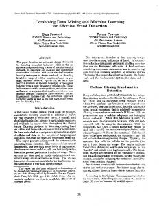
2.4 Statistical Learning Theory for Environmental Spatial Data Statistical Learning Theory (Vapnik-Chervonenkis theory) has a solid mathematical background for dependencies estimation and predictive learning from finite data sets. The workhorse of statistical learning theory – Support Vector Machines (SVM) – is based on the structural risk minimisation principle, aiming to minimise both the empirical risk and the complexity of the model, thereby providing high generalisation abilities. SVM provides non-linear classification and regression by mapping the input space into a higherdimensional feature space using kernel functions, where the optimal solutions are constructed. The theoretical details on Statistical Learning Theory and corresponding models can be found in [Vapnik, 1998]. During recent years it was shown that SVM modelling of geospatial data has a great potential, especially when data are nonlinear, high-dimensional, and noisy.
Figure 5. Support Vector Machines for geospatial data: decision function for two class spatial classification problem (white circles - support vectors) (left). Spatial regression/mapping of soil pollution data (right). It was shown that SVM has good generalisation (predictability of validation data) properties on geospatial data analysis and modelling. Examples of the results of spatial predictions (classification and mapping) using SVM are given in Figure 5. Only 56% of data are support vectors which contribute to the solution. Other data points do not contribute to the decision boundary definition. Final two-class classification is carried out by taking sign[decision_function]. An important new application of SVM for geospatial data was proposed in [Pozdnoukhov and Kanevski, 2006]. It deals with monitoring networks design/redesign based on the properties of sparseness of SVM. Only Support Vectors are important data points contributing to the solution. The task is to find potential positions of Support Vectors and to select them as a new measurement points. From the learning point of view this problem can be considered as an active learning task. An important contemporary developments concern semi-supervised or manifold learning. During following years machine learning will considerably contribute to modelling of high dimensional (geo-feature space of dimensions more than 10) nonlinear phenomena in the earth and environmental sciences. Such high-dimensional geospatial data are typical for
325
M. Kanevski, A. Pozdnoukhov, and V. Timonin / Machine Learning Algorithms for GeoSpatial Data.
topo-climatic modelling and mapping, natural hazard analysis and risk susceptibility mapping (landslides, avalanches, forest fires, etc.), assessment of renewable resources (e.g. wind-power and solar engineering). In a high dimensional space when the number of data is limited there is an important problem concerning the curse of dimensionality [Hastie et al, 2001; Haykin, 1998]. Therefore and important questions dealing with dimensionality reduction (in general nonlinear) should be considered and corresponding methods and tools selected [Lee and Verleysen, 2007]. Moreover, methods like Support Vector Machines, which are not sensitive on the dimension of the space, are preferable [Vapnik 1998]. Therefore generic methodology should be correspondingly modified taking into account the dimension of space and geo (natural) manifolds [GeoKernels, 2008, Kanevski et al., 2008].
3
SOFTWARE TOOLS
An extremely important part of intelligent data analysis using ML algorithms concerns software tools. Implementation of algorithms and development of software tools is an important step in machine learning studies. At present there are many ML software modules both commercial and freeware. Geospatial data has some specificity that can be taken into account developing corresponding modules: interactivity of training and validation, visualisation of data and analysis of the residuals, control of modelling procedures using geostatistical tools, generation of new thematic GIS layers for real decision making process etc. In [Kanevski et al., 2008] the Machine Learning Office (MLO) is presented as a complete set of tools to solve the majority of these tasks. Let us mention just some modules ands their rather unique properties: GeoMISC - utilities to perform exploratory data analysis, to manage and to visualise data and the results/residuals, generation of new GIS layers using raw data and modelling results; GeoKNN - k-Nearest Neighbour algorithm for regression and classification, training based on cross-validation, different types of Minkowski distances; GeoMLP - Multilayer Perceptron Neural Network, training using 1st and 2nd order gradient training algorithms, application of simulated annealing in order to generate starting point for the weights, different types of regularizations including noisy injection; GeoSVM - Support Vector Machines/Regression, equipped with two conventional QP solvers and tools for tuning the hyper-parameters, visualisation of support vectors; GeoGRNN - General Regression Neural Network with 6 types of kernels, cross-validation tuning of parameters, automatic detection of anisotropy; GeoGMM - Gaussian Mixture Model density estimator with full covariance matrix; GeoMDN - Mixture Density Network, based on Radial Basis Function Neural Network. GeoMDN is a valuable tool to model local probability density functions which is important for real risk mapping. An important extension of the GeoGRNN module deals with the estimation of higher moments and not only mean values and estimation of the prediction uncertainties, as well as an estimation of the validity domain which in general corresponds to the density of measurements in the input space. Software tools developed within the framework of Machine Learning Office are currently used for teaching and research in geospatial data modelling, such as topo-climatic modelling, natural hazard assessments (landslides, avalanches), pollution mapping (indoor radon, heavy metals, air and soil pollution), natural resources assessments, remote sensing images classification, socio-economic data analysis and visualisation, etc.
4.
CONCLUSIONS
Machine learning algorithms are extremely powerful adaptive, nonlinear, universal tools. They were successfully used in many geo- and environmental applications. In principle, they can be efficiently used at all stages of environmental data mining: exploratory spatial data analysis, recognition and modelling of spatio-temporal patterns, decision-oriented mapping. Current trends in ML applications for geo- and environmental sciences deal with:
326
M. Kanevski, A. Pozdnoukhov, and V. Timonin / Machine Learning Algorithms for GeoSpatial Data.
nonlinear dimensionality reduction and data visualisation; analysis and modelling of data in high-dimensional geo-feature spaces; fast modelling of physical and other processes in hybrid models; spatio-temporal patterns/structures extraction, modelling and predictions (data mining and forecasting). Finally it should be noted, that being a data driven models they need deep expert knowledge in order to be applied correctly and efficiently starting from data pre-processing to the interpretation and justification of the results.
ACKNOWLEDGEMENTS The authors wish to thank Swiss National Science Foundation (SNF) for the partial financial support of the projects “GeoKernels”(200021-113944) and “ClusterVille” (100012113506). We thank reviewers for some useful comments which helped to improve the paper.
REFERENCES Bishop, C., Patter Recognition and Machine Learning. Springer, Singapore, 2007. Cherkassky, V., V. Krasnopolsky, D. Solomatine and J. Valdes (Eds.), Special Issue: Earth Sciences and Environmental Applications of Computational Intelligence. Introduction, Neural Networks, 19(2), 111-250, 2006. Cherkassky, V., W. Hsieh, V. Krasnopolsky, D. Solomatine and J. Valdes, (Eds.), Special Issue: Computational intelligence in earth and environmental sciences. Neural Networks, 20(4), 433-558, 2007. Chiles, J.P. and P. Delfiner, Geostatistics. Modelling Spatial Uncertainty, A WileyInterscience Publication, New York, 1999. Cressie N., Statistics for spatial data, John Wiley & Sons, New-York, 1993. Haykin S., Neural Networks. A Comprehensive Foundation. Second Edition. Macmillan College Publishing Company, New York, 1998. Geokernels: http://www.geokernels.org, 2008. Hastie T., R. Tibshirani and J. Friedman, The elements of Statistical Learning. Springer, 2001. Kanevski M. and M. Maignan, Analysis and Modelling of Spatial Environmental Data. EPFL Press, Lausanne, 2004. Kanevski M., A. Pozdnoukhov and V. Timonin, Machine Learning Algorithms for Spatial Environmental Data. Applications and Software Tools. (in press), EPFL Press, Lausanne, 2008. Lee J. and M. Verleysen, Nonlinear dimensionality reduction, Springer, New York, 2007. Pozdnoukhov A. and M. Kanevski, Monitoring Network Optimisation for Spatial Data Classification Using Support Vector Machines. International Journal of Environment and Pollution, 28(3/4), 465-484, 2006. Shawe-Taylor J. and N. Cristianini, Kernel Methods for Pattern Analysis, Cambridge University Press, Cambridge, 2004. Vapnik V., Estimation of Dependencies Based on Empirical Data. Springer, New York, 1998.
327