sensors Article
Machine Learning and Computer Vision System for Phenotype Data Acquisition and Analysis in Plants Pedro J. Navarro 1, *,† , Fernando Pérez 2,† , Julia Weiss 2,† and Marcos Egea-Cortines 2,† 1 2
* †
DSIE, Universidad Politécnica de Cartagena, Campus Muralla del Mar, s/n. Cartagena 30202, Spain Genética, Instituto de Biotecnología Vegetal, Universidad Politécnica de Cartagena, Cartagena 30202, Spain;
[email protected] (F.P.);
[email protected] (J.W.);
[email protected] (M.E.-C.) Correspondence:
[email protected]; Tel.: +34-968-32-6546 These authors contributed equally to this work.
Academic Editor: Gonzalo Pajares Martinsanz Received: 3 March 2016; Accepted: 26 April 2016; Published: 5 May 2016
Abstract: Phenomics is a technology-driven approach with promising future to obtain unbiased data of biological systems. Image acquisition is relatively simple. However data handling and analysis are not as developed compared to the sampling capacities. We present a system based on machine learning (ML) algorithms and computer vision intended to solve the automatic phenotype data analysis in plant material. We developed a growth-chamber able to accommodate species of various sizes. Night image acquisition requires near infrared lightning. For the ML process, we tested three different algorithms: k-nearest neighbour (kNN), Naive Bayes Classifier (NBC), and Support Vector Machine. Each ML algorithm was executed with different kernel functions and they were trained with raw data and two types of data normalisation. Different metrics were computed to determine the optimal configuration of the machine learning algorithms. We obtained a performance of 99.31% in kNN for RGB images and a 99.34% in SVM for NIR. Our results show that ML techniques can speed up phenomic data analysis. Furthermore, both RGB and NIR images can be segmented successfully but may require different ML algorithms for segmentation. Keywords: computer vision; image segmentation; machine learning; data normalisation; circadian clock
1. Introduction The advent of the so-called omics technologies has been a major change in the way experiments are designed and has driven new ways to approach biology. One common aspect to these technology-driven approaches is the continuous decrease in price in order to achieve high throughput. As a result biology has become a field where big data accumulates, and which requires analytical tools [1]. The latest newcomer in the field of automatic sampling is the so-called phenomics. It comprises any tool that will help acquire quantitative data of phenotypes. Plant growth and development can be considered as a combination of a default program that interacts with biotic and abiotic stresses, light and temperature to give external phenotypes. And measuring, not only the outcome or end point, but also kinetics and their changes is becoming increasingly important to understand plants as a whole and become more precise at experimental designs. One of the newest developments is automatic image acquisition [2]. One of the fields where automatic image acquisition has defined its development is circadian clock analysis as promoters driving reporter genes such as luciferase or Green Fluorescent Protein allowed the identification of mutants and further characterization of the gene network at the transcriptional level [3,4]. Artificial vision systems have been used to study different aspects of plant growth and development such as root development [5], leaf growth [6], flowers and shoots [7] or seedling [8]. Sensors 2016, 16, 641; doi:10.3390/s16050641
www.mdpi.com/journal/sensors
Sensors 2016, 16, 641
2 of 16
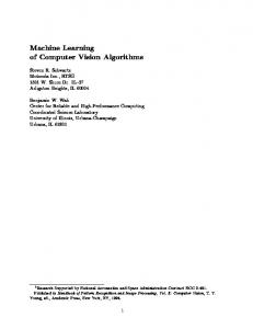
An important challenge of image acquisition in plant biology is the signalling effect of different light wavelengths including blue light, red and far red. As a result image acquisition in the dark requires Sensors 2016, 16, 641 2 of 16 infrared lightning [7,9]. Phenotyping of small plants such as Arabidopsis thaliana can be performed with a vertical camera seedling [8]. An important challenge of image acquisition in plant biology is the signalling effect of takingdifferent pictures of at time intervals orAs the parallel phenotyping several light rosettes wavelengths including blue[10]. light,Larger red andplants far red. a result image acquisition of in the traits dark require image acquisition requires infrared lightningfrom [7,9].lateral positions [11]. Thus obtaining lateral images or the reconstruction of 3-dimensional images is Arabidopsis performedthaliana by combination of cameras moving them to Phenotyping of small plants such as can be performed with aor vertical camera taking pictures of rosettes at time intervals [10]. Larger plants or the parallel phenotyping of several acquire images [12]. traits require image acquisition fromrequires lateral positions [11]. Thus obtaining lateral or the Although hardware development a multidisciplinary approach, the images bottleneck lies in reconstruction of 3-dimensional images is performed by combination of cameras or moving them to image analysis. Ideally images should be analysed in an automatic fashion. The number of images images [12]. to be acquire processed when screening populations or studying kinetics can easily go into the thousands. Although hardware development requires a multidisciplinary approach, the bottleneck lies in The partition of digital images into segments, known as segmentation is a basic process allowing the image analysis. Ideally images should be analysed in an automatic fashion. The number of images to acquisition of quantitative data that may be a number of pixels of a bidimensional field, determining be processed when screening populations or studying kinetics can easily go into the thousands. The the boundaries interest in an object [13]. known Segmentation discriminates between partition of of digital images into segments, as segmentation is a basic processbackground allowing the and defines the region under study and is the basis for further data acquision. acquisition of quantitative data that may be a number of pixels of a bidimensional field, determining The development of artificial intelligence processesdiscriminates based on machine learning (ML) the boundaries of interest in an object [13]. Segmentation between background and has the regionstep under and is the basis of for software further data been defines an important in study the development foracquision. omic analysis and modelling [14]. development artificial intelligence processes based on machine (ML) hasneighbour been Examples The include support of vector machines (SVM) for Illumina base callinglearning [15], k-nearest an important step in the development of software for omic analysis and modelling [14]. Examples (kNN) classification for protein localization [16] or Naïve Bayes Classifiers for phylogenetic include support vector machines (SVM) for Illumina base calling [15], k-nearest neighbour (kNN) reconstructions [17]. Furthermore, ML approaches have been used extensively in image analysis classification for protein localization [16] or Naïve Bayes Classifiers for phylogenetic applied to plant biology and agriculture [18,19]. reconstructions [17]. Furthermore, ML approaches have been used extensively in image analysis Plant growth occurs in aand gated manner[18,19]. i.e., it has a major peak during the late night in hypocotyls, applied to plant biology agriculture stems or large leaves [11,20,21]. This is the of circadian clock regulation of genes involved in Plant growth occurs in a gated mannerresult i.e., it has a major peak during the late night in hypocotyls, auxinstems and gibberellin signalling and cell expansion Oneclock of the inputs to circadian or large leaves [11,20,21]. This is the result of [22]. circadian regulation of the genes involvedclock in is blue light through proteins thatexpansion act as receptors as inputs ZEITLUPE/FLAVIN-BINDING, auxintransmitted and gibberellin signalling and cell [22]. Onesuch of the to the circadian clock is blueREPEAT, light transmitted through that act as receptors such as ZEITLUPE/FLAVIN-BINDING, KELCH F-BOX and LOVproteins KELCH PROTEIN2 [23,24]. Phytochromes absorb red and far red KELCH REPEAT, F-BOX and LOV KELCH PROTEIN2 [23,24]. Phytochromes absorb redwith light such as PHYTOCHROME A [25,26]. As a result night image acquisition hasred toand be far done light such as PHYTOCHROME A [25,26]. As a result night image acquisition has to be done with near infrared (NIR) light giving the so-called extended night signal [27]. The aim of this work was to near infrared (NIR) light giving the so-called extended night signal [27]. The aim of this work was to develop the corresponding algorithms to obtain data from day and night imaging. We used machine develop the corresponding algorithms to obtain data from day and night imaging. We used machine learning to analyse a set of images taken from different species during day and night. We used the learning to analyse a set of images taken from different species during day and night. We used the aforementioned SVM, NBC and kNN totoobtain Our results demonstrate aforementioned SVM, NBC and kNN obtainimage image segmentations. segmentations. Our results demonstrate that that ML has potential to tackle complex problems segmentation. MLgreat has great potential to tackle complex problemsof of image image segmentation. 2. Materials andand Methods 2. Materials Methods Figure 1a shows a schematic of of the data acquisition acquisitionsystem system is composed of four Figure 1a shows a schematic thesystem. system. The The data is composed of four modules which we describe below. modules which we describe below.
1. Growth chamber: Functionalschematic schematic of with Petunia x FigureFigure 1. Growth chamber: (a)(a) Functional of the thesystem; system;(b)(b)Experiment Experiment with Petunia x hybrida during daytime in the real system. hybrida during daytime in the real system.
2.1. Ilumination Subsystem
2.1. Ilumination Subsystem
We pursued two goals with the illumination subsystem. First we wanted to grow plants under
We pursued twotogoals with the illumination First we to growduring plantsthe under conditions close their natural environments andsubsystem. second we wanted towanted acquire pictures conditions close to their natural environments and second we wanted to acquire pictures during the
Sensors 2016, 16, 641
3 of 16
Sensors 2016, 16, 641
3 of 16
night-time without interfering with the behaviour of the plant. For this purpose, we have established night-time without interfering with the behaviour of the plant. For this purpose, we have established two illumination periods: daytime and night-time. The illumination subsystem is composed of two two illumination periods: daytime and night-time. The illumination subsystem is composed of two LED (light-emitting diode) panels which, allows to carry-out the capture image process and the same LED (light-emitting diode) panels which, allows to carry-out the capture image process and the same time it allows to supply the precise combination of the wavelengths for growing up correctly. time it allows to supply the precise combination of the wavelengths for growing up correctly. The daytime LED panel is formed by a combination of five types of LEDs emitting wavelengths The daytime LED panel is formed by a combination of five types of LEDs emitting wavelengths with peaks in UV light (290 nm), blue light (450 and 460 nm) and red light (630 and 660 nm). The LED with peaks in UV light (290 nm), blue light (450 and 460 nm) and red light (630 and 660 nm). The LED panel has a power of fifty watts. It is usually used for indoor growing of crop plants. The merging of panel has a power of fifty watts. It is usually used for indoor growing of crop plants. The merging of wavelengths produces an illumination with a pink-red appearance (Figure 2a). wavelengths produces an illumination with a pink-red appearance (Figure 2a). The night-time LED panel is composed by a bar of 132 NIR LEDs (three rows of forty four LEDs) The night-time LED panel is composed by a bar of 132 NIR LEDs (three rows of forty four LEDs) with a wavelength of 850 nm (Figure 2b). with a wavelength of 850 nm (Figure 2b). We programmed a system that would give a day/night timing whereby day light was created We programmed a system that would give a day/night timing whereby day light was created by turning on the daytime LED. In order to capture night images, the night-time LED panel was by turning on the daytime LED. In order to capture night images, the night-time LED panel was turned on for a period between 3 and 5 s coupled to an image capture trigger. The system can be turned on for a period between 3 and 5 s coupled to an image capture trigger. The system can be programmed by the user for different periods of day and night lengths and time course of picture programmed by the user for different periods of day and night lengths and time course of picture acquisition. The minimal period is one picture every 6 s and the maximal is one picture in 24 h. acquisition. The minimal period is one picture every 6 s and the maximal is one picture in 24 h.
(a)
(b)
Figure 2. Illumination subsystem (a) Daytime LED panel; (b) Nightime LED panel. Figure 2. Illumination subsystem (a) Daytime LED panel; (b) Nightime LED panel.
2.2. Capture Subsystem 2.2. Capture Subsystem The capture module is in charge of image capture during day and night and the control of the The capture module is in charge of image capture during day and night and the control of illumination subsystem. The main capture subsystem element is a multispectral 2-channel Chargethe illumination subsystem. The main capture subsystem element is a multispectral 2-channel Coupled Device (CCD) camera. A prism placed in the same optical path between the lens and CCDs Charge-Coupled Device (CCD) camera. A prism placed in the same optical path between the lens and allows a simultaneous capture the visible (or RGB) and NIR image (see Figure 3a). This feature has CCDs allows a simultaneous capture the visible (or RGB) and NIR image (see Figure 3a). This feature reduced the amount of cameras being used by the system and has avoided the construction of a has reduced the amount of cameras being used by the system and has avoided the construction mechanical system to move the lenses or the cameras in front of the plants. The camera has a of a mechanical system to move the lenses or the cameras in front of the plants. The camera has resolution of 1024 (h) × 768 (v) active pixels per channel. During day and night a resolution of 8 bit a resolution of 1024 (h) ˆ 768 (v) active pixels per channel. During day and night a resolution of 8 bit per pixel was used in all the channels (R-G-B-NIR). Figure 3b,c shows the response of the NIR-CCD per pixel was used in all the channels (R-G-B-NIR). Figure 3b,c shows the response of the NIR-CCD and RGB-CCD of the multispectral camera. and RGB-CCD of the multispectral camera. Capture and illumination subsystems are controlled via a GUI developed in C/C++ Capture and illumination subsystems are controlled via a GUI developed in C/C++ (Figure 4a,b). (Figure 4a,b). It comprises eight digital input/output channels and six analog ones in an USB-GPIO It comprises eight digital input/output channels and six analog ones in an USB-GPIO module module (Figure 5a). The system had 10 bit resolution. It was configured using the termios Linux (Figure 5a). The system had 10 bit resolution. It was configured using the termios Linux library library in C/C++. in C/C++. The second component was the optocoupler relay module. It had four optocoupled outputs, The second component was the optocoupler relay module. It had four optocoupled outputs, optocoupled to a relay triggering at voltages between 3 and 24 V. Both day light and night light LEDs optocoupled to a relay triggering at voltages between 3 and 24 V. Both day light and night light LEDs were connected to two relays (Figure 5b), in such a way that the configuration via the control software were connected to two relays (Figure 5b), in such a way that the configuration via the control software dictates the beginning of image acquisition, triggers light turning on or off coordinating the light dictates the beginning of image acquisition, triggers light turning on or off coordinating the light pulses with the camera during the day and night. pulses with the camera during the day and night.
Sensors 2016, 16, 641
4 of 16
Sensors 2016, 16, 641 Sensors 2016, 16, 641
4 of 16 4 of 16
(a) (a)
(b) (b)
(c) (c)
Figure 3. Capture subsystem (a) Prism between lens and CCDs; (b) Camera NIR-IR response; Figure 3. Capture subsystem (a) Prism between lens and CCDs; (b) Camera NIR-IR response; Figure 3. Capture subsystem (a) Prism between lens and CCDs; (b) Camera NIR-IR response; (c) Camera RGB response. (c) Camera RGB response. (c) Camera RGB response.
(a) (a)
(b) (b)
Figure 4. Graphical User Interface for capture subsystem: (a) Image control tap; (b) Time control tab. Figure 4. Graphical User Interface for capture subsystem: (a) Image control tap; (b) Time control tab. Figure 4. Graphical User Interface for capture subsystem: (a) Image control tap; (b) Time control tab.
Sensors 2016, 16, 641
5 of 16
Sensors 2016, 16, 641
5 of 16
(a)
(b)
Figure 5. Hardware of the capture subsystem. (a) USB-GPIO module (red-board) and opto-coupler Figure 5. Hardware of the capture subsystem. (a) USB-GPIO module (red-board) and opto-coupler relay relay module (green-board); (b) Electric connections between all hardware modules in the module (green-board); (b) Electric connections between all hardware modules in the growth-chamber. growth-chamber.
2.3. Image Processing Module 2.3. Image Processing Module Each experiment generates two types of images: one NIR image during the night-time and another Each experiment generates two types of images: one NIR image during the night-time and RGB image during the daytime. In order to obtain an automatic image segmentation, we designed another RGB image during the daytime. In order to obtain an automatic image segmentation, we an algorithm to classify the objects from the images of the experiment in two groups: organs and designed an algorithm to classify the objects from the images of the experiment in two groups: organs background. The algorithm developed is divided in three stages. and background. The algorithm developed is divided in three stages. 2.3.1. Extraction of Samples of Images Representative from the Different Classes 2.3.1. Extraction of Samples of Images Representative from the Different Classes During the first stage of the algorithm we have selected a set of representative samples formed by During the first stage of the algorithm we have selected a set of representative samples formed n matrix with size of k ˆ k pixels of each class. The size of the regions can be of 1 ˆ 1, 16 ˆ 16, 32 ˆ 32, by n matrix with size of k × k pixels of each class. The size of the regions can be of 1 × 1, 16 × 16, 64 ˆ 64 or 128 ˆ 128 pixels. This will depend of size and morphology of the organ to be classified and 32 × 32, 64 × 64 or 128 × 128 pixels. This will depend of size and morphology of the organ to be of the period of the daytime or night-time involved. During the day we used a single pixel per channel classified and of the period of the daytime or night-time involved. During the day we used a single while we used the larger pixel regions to increase the information obtained in the IR channel. pixel per channel while we used the larger pixel regions to increase the information obtained in the IR channel. 2.3.2. Features Vector featureVector vector is usually composed by a wide variety of different types of features. The most 2.3.2.The Features utilized features are related to: intensity of image pixels [28], geometries [29] and textures (first The feature vector is usually composed wide variety of different types of features. Theimage most and second-order statistical features) [30,31].by Inaaddition the feature vector is computed over utilized features are related to: intensity of image pixels [28], geometries [29] and textures (first transformations such as Fourier, Gabor, and Wavelet [32]. Colour images comprise three channelsand for second-order features) In addition the feature vector is the computed image R, G and B. Asstatistical a result the amount[30,31]. of information is multiplied by three and numberover of possible transformations such as Fourier, Gabor, and [32]. Colour images comprise three channels for combinations and image transformations areWavelet incremented. R, G We andhave B. Asapplied a resulttwo the amount of information is multiplied three andwhether the number of possible types of features vector techniques by depending the image was combinations and image transformations are incremented. captured during daytime (RGB image) or night-time (NIR images). We tested several colour spaces to We have appliedvector two types of features techniques depending whether the image was construct the features of daytime: RGBvector primary space, HSV perceptual space and CIE L*a*b* captured during daytime (RGB image) or night-time (NIR images). We tested several colour spaces to construct the features vector of daytime: RGB primary space, HSV perceptual space and CIE L*a*b* luminance-chrominance space [33]. The use of a single colour space produced poor results. In order
Sensors 2016, 16, 641
6 of 16
Sensors 2016, 16, 641
6 of 16
Sensors 2016, 16, 641 6 oforder 16 luminance-chrominance space [33]. The use of a single colour space produced poor results. In to to improve the performance we increased the number feature vectors.We We used used cross improve the performance we increased the number of of feature vectors. crosscombinations combinations of to the performance weand increased the number feature vectors. We used cross combinations ofimprove the RGB, CIE L*a*b*, HSV found bestofperformance was with RGB and CIE L*a*b*. the RGB, CIE L*a*b*, HSV and found that thethat bestthe performance was with RGB and CIE L*a*b*. Thus we of the RGB, CIE L*a*b*, HSV and found that the best performance was with RGB and CIE L*a*b*. Thus we constructed the features vector formed by the pixel the corresponding pixel values. In the constructed the features vector formed by the pixel the corresponding pixel values. In the NIR images, Thus we constructed featuresvector vector formed by thetwo pixel the corresponding In the NIR images, we usedthe a features computed over decomposition levels pixel of thevalues. Haar wavelet we used a features vector computed over two decomposition levels of the Haar wavelet transform. NIR images, we used a features vector computed over two decomposition levels of the Haar wavelet
transform. transform. Colour Images Colour Images Colour Imagesvector of the colour images is composed of six elements extracted from the pixel The features The features vector of the colour images is composed of six elements extracted from the pixel Theoffeatures vector of theRGB colour is We composed of asix extracted from the pixel valuesvalues of two colour spaces: RGB and CIEimages L*a*b*. selected large setset ofof random ofofeach two colour spaces: and CIE L*a*b*. We selected a elements large randompixels pixels eachclass values two colour and L*a*b*. We selected and a large set of random pixels of eachIt was to construct features vector RGB Figure 6aCIE (organs-class1-green background-class2-white). class toofthe construct the spaces: features vector Figure 6a (organs-class1-green and background-class2-white). class features vector Figure 6a (organs-class1-green and L*a*b* background-class2-white). It 6b was to necessary convert RGB colour of the original image to CIE colour L*a*b* colour necessary toconstruct converttothe RGB colour space of space the original image to CIE space. space. Figure was necessary to convert RGB colour space of the original image to CIE L*a*b* colour space. Figure 6b shows the twenty values of the features vector of class 1. shows the twenty values of the features vector of class 1. Figure 6b shows the twenty values of the features vector of class 1.
Figure 6. Colour images features vector matrixofofdifferent different pixel values corresponding Figure 6. Colour images features vectorconstruction. construction. A matrix pixel values corresponding 6.B, Colour images features vector construction. A matrix of different pixel values corresponding to R, and L*a*b* colour spaces. to R, Figure G, B, G, and L*a*b* colour spaces. to R, G, B, and L*a*b* colour spaces.
NIR Images NIR Images NIR Images Discrete Wavelet Transformation (DWT) generates a set of values formed by the “wavelet Discrete Wavelet Transformation (DWT) generates a setofofvalues values formed by the “wavelet Discrete Wavelet (DWT) generates a set formed by the “wavelet coefficients”. Being f(x,Transformation y) an image of M × N size, each level of wavelet decomposition is formed by coefficients”. Being f (x,f(x, y) anan image of MMˆ× N size,each each levelofof wavelet decomposition is formed coefficients”. Being image N size, wavelet is formed by by the convolution of the y) image f(x, y)ofwith two filters: alevel low-pass filter decomposition (LPF) and a high-pass filter the convolution of the f (x, y) twotwo filters: a low-pass (LPF) and a high-pass filter (HPF). the convolution of image the image f(x,with y)ofwith filters: a in low-pass filter (LPF) and a high-pass filter (HPF). The different combinations these filters result four filter images here described as LL, LH, HL The different combinations of these filters result in four images here described as LL, LH, HL and (HPF). The different combinations of these filters result in four images here described as LL, LH, HL and HH. In the first decomposition level four subimages or bands are produced: one smooth image, HH. ( ) and HH. In approximation, the first decomposition level four subimages or bands are produced: one smooth In thealso first decomposition level four or bands produced: one smooth image, also called ( ,subimages ), that represents an are approximation of the original imageimage, f(x, y) called ( )( ) p 1 q ( ) ( ) ( , ), that represents an approximation of the original image f(x, y) also called approximation, ( ) px, yq, approximation, f that represents an approximation of the original image f (x, y) and three , , which represent the horizontal,detail ( , ), ( , ) and and three detail subimages LL ( ) ( ) ( ) ( ) , which p 1 q p 1 q p 1 q , represent the horizontal, ( , ) , ( , ) and and three detail subimages verticalf andpx, diagonal respectively. There are represent several wavelet mother functions be yq, f HL details px, yq and subimages f HH px, yq, which the horizontal, verticalthat andcan diagonal LH diagonal vertical and details respectively. There are several wavelet mother functions can be employed, like Haar, Daubechies, Coiflet, Meyer, Morlet, and Bior, depending on that the specific details respectively. There are several wavelet mother functions that can be employed, like Haar, employed, Haar, Daubechies, Coiflet, Meyer, Morlet, and Bior, depending on the specific problem to like be identified [34,35]. Figure 7 shows the pyramid algorithm of wavelet transform in the Daubechies, Coiflet, Meyer, Morlet, and Bior, depending on thealgorithm specific problem to transform be identified [34,35]. problem to be identified [34,35]. Figure 7 shows the pyramid of wavelet in the first decomposition level. Figure 7 shows the pyramid first decomposition level. algorithm of wavelet transform in the first decomposition level.
Figure 7. First level of direct 2D-DWT decomposition. Figure 7. First level of direct 2D-DWT decomposition.
Figure 7. First level of direct 2D-DWT decomposition.
In this work we have computed a features vector based on the wavelet transform with basis Haar [36]. The features vector is formed of four elements: maximum, minimum, mean and Shannon
Sensors 2016, 16, 641
7 of 16
entropy of coefficients wavelets calculated in the horizontal, vertical and diagonal subimages in two decomposition levels (see Equations (1)–(5)): We have eliminated the approximation subimage due to it contains a representation decimated of the original image: f 1,
f 19,
.., 6
! ) pl q pl q pl q “ max f LH px, yq , f LH px, yq , f LH px, yq , @l “ 1, 2
! ) pl q pl q pl q f 7,..,12 “ min f LH px, yq , f LH px, yq , f LH px, yq , @l “ 1, 2 ) ! pl q pl q pl q f 13,..,18 “ mean f LH px, yq , f LH px, yq , f LH px, yq , @l “ 1, 2 ! ) pl q pl q pl q ..,24 “ shannon_entropy f LH px, yq , f LH px, yq , f LH px, yq , @l “ 1, 2
(1) (2) (3) (4)
Shannon Entropy is calculated as the Equation (5): ´ shannon_entropy
pl q fs
M {2l Nÿ {2l ÿ
¯ “´
` ˘ ` ` ˘˘ p wij log2 p wij
(5)
i “1 j “1
The letter l represents the value of the wavelet decomposition level, s the subimages (LL, HL, LH, HH) created in the wavelet decomposition, and wij represents the wavelet coefficient (i, j), located in the s-subimage, at l-decomposition level. p represents the occurrence probability of the wavelet coefficient wij . Feature vector has been obtained applying the Equations (1)–(5) to each region in two wavelet decomposition levels with Haar basis. The result was a feature vector of twenty-four elements ( f 1,..,24 ) per region of size k ˆ k. 2.3.3. Classification Process We have tested three machine-learning algorithms: (1) k-nearest neighbour (kNN); (2) naive Bayes classifier (NBC), and Support Vector Machine (SVM). The algorithms selected belong to the type of supervised classification. These type of algorithms require of a training stage before performing the classification process. kNN classifier is a non-parametric method for classifying objects in a multi-dimensional space. After being trained, kNN assigns a specific class to a new object depending on the majority of votes from its neighbours. This measure is based in metrics such as Euclidean, Hamming or Mahalanobis distances. In the implementation of kNN algorithm it is necessary to assign an integer value to k. This parameter represents the k-neighbors used to carry-out the voting classification. A k optimal determination will allow that the good model adjusts to future data [37]. It is recommendable to use data normalisation coupled to kNN classifiers in order to avoid the predominance of big values over small values in the features vector. NBC uses a probabilistic learning classification. Classifiers based on Bayesian methods utilize training data to calculate an observed probability of each class based on feature values. When the classifier is used later on unlabeled data, it uses the observed probabilities to predict the most likely class for the new features. As NBC works with probabilities it does not need data normalization. SVM is a supervised learning algorithm where given labeled training data, it outputs a boundary which divides data by categories and categorizes new examples. The goal of a SVM is to create a boundary, called hyperplane, which leads to homogeneous partitions of data on either side. SVMs can also be extended to problems were the data are not linearly separable. SVMs can be adapted for use with nearly any type of learning task, including both classification and numeric prediction. SVM classifier tend to perform better after data normalisation. In this work we have used raw data and two types of normalisation procedures which have been computed over features space: dn0: without normalisation; dn1: mean and standard-deviation
Sensors 2016, 16, 641
8 of 16
normalization and dn2: mode and standard-deviation normalisation. Features space of each class is composed by a m ˆ n matrix (see Equation (6)): »
f ijnC
1 f 11 .. . 1 f 1m
— — — — — — — — “— — — — — — — — –
nC f 11 .. . nC f 1m
¨¨¨ .. . ¨¨¨ ¨ ¨ ¨ ¨¨¨ .. . ¨¨¨
fi
1 f 1n .. . 1 f mn
ffi ffi ffi ffi ffi ffi ffi ffi ffi ∇ i “ 1, . . . , m ; j “ 1, . . . , n ; nC “ 1, 2 ffi ffi ffi ffi ffi ffi ffi fl
nC f 1n .. . nC f mn
(6)
Being i-th row, the vector of features i-th of features space formed by n features. m represents the number of vectors in the features space and nC represents the number of classes in th space. The normalised features space, Fijnc , depending on the normalisation types (dn0, dn1, dn2) is computed as is shown in the Equation (7): »
Fijnc
— — — — — — — — — — “— — — — — — — — — –
1 ´st f 11 1 st2
.. .
1 ´st f 1m 1 st2
nC ´st f 11 1 st2
.. .
nC ´st f 1m 1 st2
¨¨¨ .. . ¨¨¨ ¨ ¨ ¨ ¨¨¨ .. . ¨¨¨
1 ´st f 1n 1 st2
.. .
1 ´st f mn 1 st2
nC ´st f 1n 1 st2
.. .
nC ´st f mn 1 st2
fi ffi ffi ffi $ # ffi ’ st1 “ 0 ’ ffi ’ dn0 raw data ’ ffi ’ ’ ffi st2 “ 1 ’ ’ ffi # ’ & ffi st1 “ meanp f ijnC q ffi dn1 Ñ ffi ’ ffi st “ StdDesp f ijnC q ’ ’ ffi # 2 ’ ’ ffi ’ st1 “ modep f ijnC q ’ ffi ’ dn2 ’ ffi % ffi st2 “ StdDesp f ijnC q ffi ffi fl
(7)
To obtain the best result in classification process, the ML algorithms were tested with different configuration parameters. kNN was tested with Euclidean and Minkowski distances with three type of data normalisation, NBC was tested with Gauss and Kernel Smoothing Functions (KSF) without data normalisation, and SVM was tested with linear and quadratic functions, on three types of data normalisation. The ML algorithms used two classes of objects. One for the plant organs and a second one for the background. In all of them we applied the leave-out cross validation (LOOCV) method to measure of the error of the classifier. Basically LOOCV method extracts a sample of the training set and it constructs the classifier with the remaining of the training samples. Then it evaluates the classification error and the process is repeated for all the training samples. At end the LOOCV method computes the mean of the errors and it obtains a measure of how model is adjusted to data. This method allows comparing the results of the different ML algorithms, provided that they will be applied to same sample data. Table 1 shows a summary of parameters used for the classification process. Table 1. kNN, NBC and SVM configuration parameters. Configuration
kNN
NBC
SVM
method data normalisation metrics classes
Euclidean, Minkowski dn0, dn1, dn2 LOOCV, ROC 2
Gauss, KSF dn0 LOOCV, ROC 2
Linear, quadratic dn1, dn2 LOOCV, ROC 2
Sensors 2016, 16, 641
9 of 16
2.4. Experimental Validation In order to test and validate the functioning of the system and ML methods, acquired pictures of Antirrhinum majus and Antirrhinum linkianum were used to analyse growth kinetics. The camera was positioned above the plants under study. The daylight LED panel was above the plants while the night-time LED was at a 45˝ . Data acquisition was performed for a total of six days. We obtained one image every 10 min during day and night. Day night cycles were set to 12:12 h and triggering of the 2016, 16, 641 9 of 16 NIR LEDSensors for image acquisition during the night was done for a total of 6 s. In the experiment we obtained 864 colour images from the RGB sensor which were transformed obtained one image every 10 min during day and night. Day night cycles were set to 12:12 h and to CIE L*a*b* colour andfor864 gray scale images thewas NIR sensor. From group (RGB triggering of thespace NIR LED image acquisition during from the night done for a total of 6each s. In the we experiment we fifty obtained 864 colour images from the RGB sensor which weremanually transformed and NIR images) obtained ground-truth images which were segmented by human CIE L*a*b* colour space and 864colour gray scale imageswe from the NIR 1200 sensor.samples From each (RGB experts. to From the fifty ground-truth images, selected ofgroup 1 pixel, which we and NIR images) we obtained fifty ground-truth images which were segmented manually by human used to train the RGB image processing ML algorithms. From the second fifty ground-truth NIR experts. From the fifty ground-truth colour images, we selected 1200 samples of 1 pixel, which we images we 1200 of 32 ˆ 32 pixels which were train thefifty NIRground-truth image processing ML usedtook to train theregions RGB image processing ML algorithms. Fromtothe second NIR algorithms. In both cases we selected 600 samples belonging to organs class and 600 samples belonging images we took 1200 regions of 32 × 32 pixels which were to train the NIR image processing ML algorithms. In both cases we selected 600 samples belonging to organs class and 600 samples to background class. belonging to background class. Figure 8 shows two images from each day of the experiment for different capture periods. We can Figure 8 shows two images from each day of the experiment for different capture periods. We distinguish easily the growth stages of the two species during the daytime and night-time. can distinguish easily the growth stages of the two species during the daytime and night-time.
Day1
Night1
Day2
Night2
Day3
Night3
Day4
Night4
Day5
Night5
Day6
Night6
Figure 8. Images of the experiment captured every 12 h.
Figure 8. Images of the experiment captured every 12 h. 3. Results and Discussion
3. Results and We Discussion evaluated the results of training stage of the ML algorithms with a leave-one-out crossvalidation method (LOOCV) and with the Receiver Operating Characteristic (ROC) curve over data
We evaluated the results of training stage of the ML algorithms with a leave-one-out training sets obtained from RGB and NIR images. LOOCV and ROC curves have been applied under cross-validation method (LOOCV) shown and with Receiver Operating Characteristic curve over the different ML configurations in thethe Table 1. This allowed to select the optimal ML(ROC) algorithm data training obtained anddepending NIR images. LOOCV and ROC curves been to be sets applied to eachfrom type RGB of image on when it was captured: during have daytime or applied night-time. determined the shown optimal ML algorithm each image set, we used the metric under the differentOnce MLwe configurations in the Table for 1. This allowed to select the optimal ML miss-classification [37] to evaluate final performance thewhen implemented ML algorithms. algorithm to be applied to each type ofthe image dependingofon it was captured: during daytime or night-time. Once we determined the optimal ML algorithm for each image set, we used the metric 3.1. LOOCV miss-classification [37] to evaluate the final performance of the implemented ML algorithms.
Table 2 shown the errors obtained after to apply LOOCV to the two images groups respectively. In both images groups the minimum error in data model adjust is produced with kNN classifier. Data 3.1. LOOCV normalisation based on in the mean (dn1) produced the best result in both cases, too. The maximum error is produced by the NBC classifier, with and LOOCV Gauss kernel, respectively. Table 2 shown the errors obtained after toKSF apply to the two images groups respectively.
In both images groups the minimum error in data model adjust is produced with kNN classifier. Data normalisation based on in the mean (dn1) produced the best result in both cases, too. The maximum error is produced by the NBC classifier, with KSF and Gauss kernel, respectively.
Sensors 2016, 16, 641
10 of 16
Table 2. Colour images and NIR images. LOOCV error for kNN, NBC, SVM. Sensors 2016, 16, 641
10 of 16
Classifier kNN NBC SVM Table 2. Colour images and NIR images. LOOCV error for kNN, NBC, SVM. Configuration Euclidean Minkowski Gauss KSF Linear Quadratic
Classifier dn0 dn1 Colour Configuration dn2 dn0 Colour dn1 dn0 dn1 NIR dn2 dn2 dn0 NIR dn1 3.2. ROC Curves dn2
0.0283 kNN 0.0433 0.0242 0.0467 Euclidean Minkowski 0.0283 0.0433 0.0283 0.0433
0.0242 0.0288 0.0169 0.0283 0.0288 0.0288 0.0169 0.0288
0.0467 0.0394, 0.0281 0.0433 0.0394 0.0394, 0.0281 0.0394
NBC 0.0758 0.0750 Gauss KSF 0.0750 0.0758
SVM 0.0533 0.0383 Linear Quadratic 0.0667 0.0450 -
0.0356 -0.0356
0.0319 0.0319
0.0533 0.0326 0.0667 0.0344 -
0.0383 0.0319 0.0450 0.0325 -
-
-
0.0326 0.0344
0.0319 0.0325
We evaluated the performance of the ML algorithms using Receiver Operating Characteristic 3.2. ROC Curves (ROC) curve. The ROC curve is created by comparing the sensitivity (the rate of true positives TP, see We(8)), evaluated the performance of the using Characteristic Equation versus 1-specificity (the rate of ML falsealgorithms positives FP see Receiver EquationOperating (9)), at various threshold (ROC) curve. The ROC curve is created by comparing the sensitivity (the rate of true positives levels [38]. The ROC curves, shown in Figures 8 and 9 allow comparing the results between ofTP, ML see Equation (8)), groups versus 1-specificity algorithms per each of images: (the rate of false positives FP see Equation (9)), at various threshold levels [38]. The ROC curves, shown in Figures 8 and 9, allow comparing the results between TP of ML algorithms per each groups of images: (8) Sensitivity “ TP ` FN (8) = + TN Speci f icity “ (9) TN ` FP (9) = The Area Under the Curve (AUC) is usually used by + ML to compare statistical models. AUC can
1
1
0.95
0.95
0.9
KNN dn0 euclidean KNN dn1 euclidean KNN dn2 euclidean
Sensitivity
Sensitivity
The Area the Curve (AUC) is usually used ML to acompare AUC can be interpreted asUnder the probability that the classifier willbyassign higher statistical score to amodels. randomly chosen be interpreted as the probability that the classifier will assign a higher score to a randomly chosen positive example than to a randomly chosen negative example [39,40]. positive a randomly chosen negative Figureexample 9 shows than ROCtocurves computed over the set example of colour[39,40]. images training. The higher values of Figure 9 shows ROC curves computed over the set of colour images training. higher valueswe AUC were obtained by kNN classifier with Euclidean distance. Concerning the dataThe normalisation, of AUC were obtained by kNN classifier with Euclidean distance. Concerning the data normalisation, achieved similar results with raw data and normalisation based on the mode and standard deviation we achieved similar results with raw data and normalisation based on the mode and standard (dn0 and dn1). deviation (dn0 and dn1). Figure 10 shows ROC curves computed over the set of NIR images training. We can observe that Figure 10 shows ROC curves computed over the set of NIR images training. We can observe that the best results were obtained with the SVM classifier with quadratic functions and using a normalised the best results were obtained with the SVM classifier with quadratic functions and using a data based on the mean and standard deviation (dn1). Table 3 shows AUC values obtained from ROC normalised data based on the mean and standard deviation (dn1). Table 3 shows AUC values curves of thefrom Figures and 10. obtained ROC9curves of the Figures 9 and 10. In In both cases after postprocessingstage stagecomposed composedofof both cases afterclassification classificationstages, stages, we we performed performed aa postprocessing morphological operations small particles. particles.The Thesegmented segmented morphological operationsand andan anarea areafilter filterto toeliminate eliminate noise noise and and small images were merged with the original images (Figures 11 and 12). images were merged with the original images (Figures 11 and 12).
0.9
0.85
0.85
0.8
0.8
0
0.05
0.1
1-Specificity
0.15
0.2
KNN dn0 minkowski KNN dn1 minkowski KNN dn2 minkowski
0
(a)
0.05
0.1
1-Specificity
(b) Figure9. 9. Cont. Cont. Figure
0.15
0.2
Sensors 2016, 16, 641 Sensors 2016, 16, 641 Sensors 2016, 16, 641 11
1
0.8
0.8
0.8 0.8
0.7
0.7
0.7 0.7
0.6
0.6 0.6
0.5 0.4
Sensitivity Sensitivity
0.9
0.6
NBC dn0 Gauss NBC dn0 Gauss NBC dn0 KSF NBC dn0 KSF
0.5
0.5 0.5 0.4 0.4
0.4 0.3
0.3 0.3
0.2
0.2 0.2
0.1
0.1 0.1
0.3 0.2 0.1
0
0 0
0
SVM dn1 Poly 1 1 SVM dn1 Poly SVM dn2 Poly 1 1 SVM dn2 Poly SVM dn1 Poly 2 2 SVM dn1 Poly SVM dn2 Poly 2 2 SVM dn2 Poly
0.9 0.9
0.9
Sensitivity
Sensitivity
1
11 of 16 1111 ofof 1616
0
0.1
0.1
0.2
0.2
0.3
0.3
0.4
0.4
0.5
0.6
0.7
1-Specificity 0.5 0.6
0.7
1-Specificity
0.8
0.8
0.9
1
0.9
0
0
0
1
0.1
0.2
0.3
0.1
0.2
0.3
(c)
0.4
0.5
0.6
0.7
1-Specificity 0.4 0.5 0.6
0.8
0.7
1-Specificity
0.9
0.8
1
0.9
1
(d)
(c)
(d)
Figure 9. ROC results for training colour images. (a) kNN classifier with distance Euclidean and data Figure 9. 9. ROC ROCresults resultsfor for training colour colour images. images. (a) (a)kNN kNNclassifier classifierwith withdistance distanceEuclidean Euclidean and and data data Figure normalisation: dn0, dn1training and dn2; (b) kNN classifier with distance Minkowski and data normalisation: normalisation: dn0, dn1 and dn2; (b) kNN classifier with distance Minkowski and data normalisation: normalisation: andclassifier dn2; (b) with kNNGauss classifier distanceand Minkowski and data normalisation: dn0, dn1 anddn0, dn2;dn1 (c) BN andwith KSF kernels data normalisation dn0; (d) SVM dn0, dn1 dn1 and and dn2; dn2; (c) (c)BN BNclassifier classifier with with Gauss Gauss and and KSF KSF kernels kernels and and data data normalisation normalisation dn0; dn0; (d) (d) SVM SVM dn0, classifier with lineal and quadratic polynomial functions and data normalisation: dn1 and dn2. classifier with with lineal lineal and and quadratic quadratic polynomial polynomial functions functions and and data data normalisation: normalisation: dn1 dn1 and and dn2. dn2. classifier 1
1
1
1
0.95
0.95
Sensitivity
Sensitivity
0.9
KNN dn0 euclidean KNN dn1 euclidean KNN dn2 euclidean
0.9
KNN dn0 euclidean KNN dn1 euclidean KNN dn2 euclidean
0.85
Sensitivity Sensitivity
0.95
0.95
0.9
0.8
0.8
0.8
0.8 0
0.05
0
0.1
1-Specificity
0.05
(a)
0.1
1-Specificity
0.15
0
0.2
0.15
0.1
1-Specificity
0.15
(b) 0.1
0.05
1-Specificity
0.2
0.15
0.2
(b)
1
SVM dn1 Poly 1 SVM dn2 Poly 1 SVM dn1 Poly 2 SVM dn2 Poly 2
0.9
0.9
1
1 0.8
0.8
0.7
0.9 0.7
0.6
0.8 0.6
Sensitivity
0.8
0.5
0.7 0.5
NBC dn0 Gauss NBC dn0 KSF
0.5
0.6 0.4
0.4
NBC dn0 Gauss NBC dn0 KSF
0.3
0.5 0.3
0.4
0.2
0.4 0.2
0.3
0.1
0.3 0.1
0.2
0
0.20 0
0.1
0.2
0.3
0.4
0.5
0.6
0.7
1-Specificity
0.1
0.8
0.9
0.1
0.2
0.3
0.4
0.5
0
1
0.1
0.2
0.3
0.1
0.2
0.3
0.1
(c)
0 0
SVM dn1 Poly 1 SVM dn2 Poly 1 SVM dn1 Poly 2 SVM dn2 Poly 2
SensitivitySensitivity
0.9
Sensitivity
0.05
0
0.2
(a)
1
0.6
KNN dn0 minkowski KNN dn1 minkowski KNN dn2 minkowski
0.85
0.85
0.85
0.7
KNN dn0 minkowski KNN dn1 minkowski KNN dn2 minkowski
0.9
0.4
0.7
0.8
0.9
1
0.6
0.7
0.8
0.9
1
(d)
0
0.6
0.5
1-Specificity
0
0.4
0.5
0.6
0.7
0.8
0.9
1-Specificity 1-Specificity Figure 10. ROC results for training NIR images. (a) kNN classifier with distance Euclidean and data (d) data normalisation: normalisation: dn0,(c) dn1 and dn2; (b) kNN classifier with distance Minkowski and dn0, dn1 and dn2; (c) BN classifier with Gauss and KSF kernels and data normalisation dn0; (d) SVM Figure 10. ROC results for training NIR images. (a) kNN classifier with distance Euclidean and data Figure 10. ROC for quadratic training NIR images.functions (a) kNN and classifier with distancedn1 Euclidean and data classifier with results lineal and polynomial data normalisation: and dn2. normalisation: dn0, dn1 and dn2; (b) kNN classifier with distance Minkowski and data normalisation: normalisation: dn0, dn1 and dn2; (b) kNN classifier with distance Minkowski and data normalisation: dn0, dn1 and dn2; (c) BN classifier with Gauss and KSF kernels and data normalisation dn0; (d) SVM dn0, dn1 and dn2; (c) BN classifier with Gauss and KSF kernels and data normalisation dn0; (d) SVM classifier with lineal and quadratic polynomial functions and data normalisation: dn1 and dn2. classifier with lineal and quadratic polynomial functions and data normalisation: dn1 and dn2.
1
Sensors 2016, 16, 641
12 of 16
Sensors 2016, 16, 641 Sensors 2016, 16, 641
Table 3. Colour images and NIR images. AUC for kNN, NBC, SVM. Table 3. Colour images and NIR images. AUC for kNN, NBC, SVM. Table 3. Colour images and NIR images. AUC for kNN, NBC, SVM. Classifier kNN NBC Classifier kNN NBC
Classifier kNN Configuration Configuration Euclidean Euclidean Minkowski Minkowski Configuration Euclidean Minkowski dn0 0.9984 0.9974 dn0 0.9984 0.9974 dn0 0.9984 0.9974 Colour dn1 0.9979 0.9976 dn1 0.9979 0.9976 Colour Colour dn1 0.9979 0.9976 dn2 0.9984 0.9974 dn2 0.9984 0.9974 dn2 0.9984 0.9974 dn0 0.9987 0.9979 dn0 0.9987 0.9979 dn0 0.9987 0.9979 NIR dn1 0.9975 0.9993 dn1 0.9975 0.9993 NIR NIR dn1 0.9975 0.9993 dn2 0.9987 0.9979 dn2 0.9987 0.9979 dn2 0.9987 0.9979
NBC Gauss KSF Gauss KSF Gauss KSF 0.9542 0.9778 0.9542 0.9778 0.9542 0.9778 - --- --0.9877 0.9963 0.9877 0.9963 0.9877 0.9963 - --- ---
12 of 16 12 of 16
SVM SVM
Linear Linear
Linear -0.9622 0.9622 0.9622 0.9496 0.9496 0.9496 -0.9867 0.9867 0.9867 0.9868 0.9868 0.9868
SVM Quadratic Quadratic Quadratic - 0.9875 0.9875 0.9875 0.9886 0.9886 0.9886 - 1.000 1.000 1.000 0.9932 0.9932 0.9932
Figure 11. Results of the colour image segmentation based on kNN classifier in different growing Figure 11.11.Results ofofthe colour image segmentation based on on kNNclassifier classifierinindifferent different growing Figure the colour image segmentation based growing stages. Left Results shows four colour images selected at different growthkNN stages. The second column presents stages. Left shows four colour images selected at different growth stages. The second column presents stages. Leftofshows four colour images at different growthdistance stages. The column presents the result segmentation using kNNselected classifier with Euclidean andsecond without normalisation thethe result of segmentation using kNN classifier with Euclidean distance and without normalisation segmentation using kNN withpost-processing Euclidean distance dataresult (dn0).ofThe third column shows theclassifier results after stage.and without normalisation data (dn0). The third stage. data (dn0). The thirdcolumn columnshows showsthe theresults results after after post-processing post-processing stage.
Figure 12. Results of the NIR image segmentation based on SVM. Left shows four NIR images chosen Figure Results theNIR NIR imagesegmentation segmentation based on Left shows four images chosen Figure 12.12. Results ofofthe image basedThe on SVM. SVM. Left shows fourNIR NIR images chosen at different growth stages growing during night-time. second column shows the segmentation at different growth stages growing during night-time. The second column shows the segmentation after application the SVM classifier with quadratic function and with datathe normalisation at results different growth stagesof growing during night-time. The second column shows segmentation results after application of thethe SVM classifier with quadratic stage. function and with data normalisation dn1. The third columnof shows after post-processing results after application the SVMresults classifier with quadratic function and with data normalisation dn1. dn1. The third column shows the results after post-processing stage. The third column shows the results after post-processing stage.
Sensors 2016, 16, 641
13 of 16
3.3. Error Segmentation The misclassification error (ME) represents the percentage of the background pixels that are incorrectly allocated to the object (i.e., to the foreground) or vice versa. The error can be calculated by means of Equation (10), where BGT (Background Ground-Truth image) and OGT (Object Ground-Truth image) represent the ground-truth image of the background and of the object taken as reference, and BT (Background Test) and OT (Object Test) represent the image to be assessed. In the event that the test image coincides with the pattern image, the classification error will be zero and therefore the performance of the segmentation will be the maximum [41]. ME “
|BGT X BT | ` |OGT X OT | |BGT | ` |OGT |
(10)
The performance of the implemented algorithms is assessed according to the Equation (11): η “ 100¨ p1 ´ MEq
(11)
Table 4 shows mean values computed after to segment the fifty ground-truth images of each group with optimal ML algorithm (kNN and SVM) selected in the previous subsection. Table 4. Performance in the image segmentation. Classifier
kNN
SVM
Performance
99.311%
99.342%
The performance of the image segmentation calculated shows excellent results in both groups (Table 4). It has been necessary to increase the complexity of the features vector in the NIR images (using Wavelet transform) to obtain a similar results of performance. This is probably an expected result as RGB images had three times more of information than a NIR image. 4. Conclusions and Future Work In this work we have developed a system based on ML algorithms and computer vision intended to solve the automatic phenotype data analysis. The system is composed by a growth-chamber with capacities to perform experiments with numerous species. The design of the growth-chamber has allowed easy positioning of different cameras and illuminations. The system can take thousands of images through the capture subsystem, capture spectral images and it creates time-lapse series of the specie during the experiment. One of the main goals of this work has been to capture images during the night-time without affecting plant growth. We have used three different ML algorithms for image segmentation: k-nearest neighbour (kNN), Naive Bayes classifier (NBC), and Support Vector Machine. Each ML algorithm was executed with different kernel functions: kNN with Euclidean and Minkowski distances, NBC with Gauss and KSF functions and SVM with linear and quadratic functions. Furthermore ML algorithms have been trained with two types of data normalisation: dn0 (raw data), dn1 (mean and standard deviation) and dn2 (mode & standard deviation). Our results show that RGB images are better classified with the kNN classifier, Euclidean distance and without data normalisation. In contrast, NIR images performed better with SVM classifier with quadratic function and with data normalisation dn1. In the last stage we have applied ME metrics to measure the image segmentation performance. We have achieved a performance of 99.3% in both ground-truth colour images and ground-truth NIR images. Currently the algorithms are being used in an automatic image segmentation processing to study circadian rhythm in wild type lines, transposon-tagged mutants and transgenic lines with modifications in genes involved in the control of growth and the circadian clock. Regarding future work, we consider important to identify a new feature vector which produces better performance rates,
Sensors 2016, 16, 641
14 of 16
improve the illumination subsystem, reduce the computation time of the windowing segmentation in NIR images. Acknowledgments: The work has been partially supported and funded by the Spanish Ministerio de Economía y Competitividad (MINECO) under the projects ViSelTR (TIN2012-39279), BFU2013-45148-R and cDrone (TIN2013-45920-R). Author Contributions: Pedro J. Navarro, Fernándo Pérez, Julia Weiss and Marcos Egea-Cortines conceived and designed the experiments; Pedro J. Navarro, Fernándo Pérez, Julia Weiss, and Marcos Egea-Cortines performed the experiments; Pedro J. Navarro and Fernándo Pérez analyzed the data; Julia Weiss contributed reagents/materials/analysis tools; Pedro J. Navarro, Fernándo Pérez and Marcos Egea-Cortines wrote the paper. Pedro J. Navarro, Fernándo Pérez, Julia Weiss and Marcos Egea-Cortines corrected the draft and approved the final version. Conflicts of Interest: The authors declare no conflict of interest.
Abbreviations The following abbreviations are used in this manuscript: LM KSF kNN NBC SVM LOOCV AUC ME
Machine learning Kernel smoothing function k-nearest neighbour Naïve Bayes classifier Support vector machines Leave-one-out cross validation method Area under curve Misclassification error
References 1. 2. 3. 4. 5. 6.
7. 8. 9. 10. 11.
12.
Fahlgren, N.; Gehan, M.; Baxter, I. Lights, camera, action: High-throughput plant phenotyping is ready for a close-up. Curr. Opin. Plant Biol. 2015, 24, 93–99. [CrossRef] [PubMed] Deligiannidis, L.; Arabnia, H. Emerging Trends in Image Processing, Computer Vision and Pattern Recognition; Elsevier: Boston, MA, USA, 2014. Dee, H.; French, A. From image processing to computer vision: Plant imaging grows up. Funct. Plant Biol. 2015, 42, iii–v. [CrossRef] Furbank, R.T.; Tester, M. Phenomics—Technologies to relieve the phenotyping bottleneck. Trends Plant Sci. 2011, 16, 635–644. [CrossRef] [PubMed] Dhondt, S.; Wuyts, N.; Inzé, D. Cell to whole-plant phenotyping: The best is yet to come. Trends Plant Sci. 2013, 18, 428–439. [CrossRef] [PubMed] Tisné, S.; Serrand, Y.; Bach, L.; Gilbault, E.; Ben Ameur, R.; Balasse, H.; Voisin, R.; Bouchez, D.; Durand-Tardif, M.; Guerche, P.; et al. Phenoscope: An automated large-scale phenotyping platform offering high spatial homogeneity. Plant J. 2013, 74, 534–544. [CrossRef] [PubMed] Li, L.; Zhang, Q.; Huang, D. A review of imaging techniques for plant phenotyping. Sensors 2014, 14, 20078–20111. [CrossRef] [PubMed] Honsdorf, N.; March, T.J.; Berger, B.; Tester, M.; Pillen, K. High-throughput phenotyping to detect drought tolerance QTL in wild barley introgression lines. PLoS ONE 2014, 9, 1–13. [CrossRef] [PubMed] Barron, J.; Liptay, A. Measuring 3-D plant growth using optical flow. Bioimaging 1997, 5, 82–86. [CrossRef] Aboelela, A.; Liptay, A.; Barron, J.L. Plant growth measurement techniques using near-infrared imagery. Int. J. Robot. Autom. 2005, 20, 42–49. [CrossRef] Navarro, P.J.; Fernández, C.; Weiss, J.; Egea-Cortines, M. Development of a configurable growth chamber with a computer vision system to study circadian rhythm in plants. Sensors 2012, 12, 15356–15375. [CrossRef] [PubMed] Nguyen, T.; Slaughter, D.; Max, N.; Maloof, J.; Sinha, N. Structured light-based 3d reconstruction system for plants. Sensors 2015, 15, 18587–18612. [CrossRef] [PubMed]
Sensors 2016, 16, 641
13. 14. 15. 16. 17.
18. 19. 20. 21.
22. 23.
24.
25. 26. 27.
28.
29. 30. 31. 32. 33.
34.
15 of 16
Spalding, E.P.; Miller, N.D. Image analysis is driving a renaissance in growth measurement. Curr. Opin. Plant Biol. 2013, 16, 100–104. [CrossRef] [PubMed] Navlakha, S.; Bar-joseph, Z. Algorithms in nature: The convergence of systems biology and computational thinking. Mol. Syst. Biol. 2011, 7. [CrossRef] [PubMed] Kircher, M.; Stenzel, U.; Kelso, J. Improved base calling for the Illumina Genome Analyzer using machine learning strategies. Genome Biol. 2009, 10, 1–9. [CrossRef] [PubMed] Horton, P.; Nakai, K. Better prediction of protein cellular localization sites with the k nearest neighbors classifier. Proc. Int. Conf. Intell. Syst. Mol. Biol. 1997, 5, 147–152. [PubMed] Yousef, M.; Nebozhyn, M.; Shatkay, H.; Kanterakis, S.; Showe, L.C.; Showe, M.K. Combining multi-species genomic data for microRNA identification using a Naive Bayes classifier. Bioinformatics 2006, 22, 1325–1334. [CrossRef] [PubMed] Tellaeche, A.; Pajares, G.; Burgos-Artizzu, X.P.; Ribeiro, A. A computer vision approach for weeds identification through Support Vector Machines. Appl. Soft Comput. J. 2011, 11, 908–915. [CrossRef] Guerrero, J.M.; Pajares, G.; Montalvo, M.; Romeo, J.; Guijarro, M. Support Vector Machines for crop/weeds identification in maize fields. Expert Syst. Appl. 2012, 39, 11149–11155. [CrossRef] Covington, M.F.; Harmer, S.L. The circadian clock regulates auxin signaling and responses in Arabidopsis. PLoS Biol. 2007, 5, 1773–1784. [CrossRef] [PubMed] Nusinow, D.A.; Helfer, A.; Hamilton, E.E.; King, J.J.; Imaizumi, T.; Schultz, T.F.; Farré, E.M.; Kay, S.A.; Farre, E.M. The ELF4-ELF3-LUX complex links the circadian clock to diurnal control of hypocotyl growth. Nature 2011, 475, 398–402. [CrossRef] [PubMed] De Montaigu, A.; Toth, R.; Coupland, G. Plant development goes like clockwork. Trends Genet. 2010, 26, 296–306. [CrossRef] [PubMed] Baudry, A.; Ito, S.; Song, Y.H.; Strait, A.A.; Kiba, T.; Lu, S.; Henriques, R.; Pruneda-Paz, J.L.; Chua, N.H.; Tobin, E.M.; et al. F-box proteins FKF1 and LKP2 Act in concert with ZEITLUPE to control arabidopsis clock progression. Plant Cell 2010, 22, 606–622. [CrossRef] [PubMed] Kim, W.-Y.Y.; Fujiwara, S.; Suh, S.-S.S.; Kim, J.; Kim, Y.; Han, L.Q.; David, K.; Putterill, J.; Nam, H.G.; Somers, D.E. ZEITLUPE is a circadian photoreceptor stabilized by GIGANTEA in blue light. Nature 2007, 449, 356–360. [CrossRef] [PubMed] Khanna, R.; Kikis, E.A.; Quail, P.H. EARLY FLOWERING 4 functions in phytochrome B-regulated seedling de-etiolation. Plant Physiol. 2003, 133, 1530–1538. [CrossRef] [PubMed] Wenden, B.; Kozma-Bognar, L.; Edwards, K.D.; Hall, A.J.W.; Locke, J.C.W.; Millar, A.J. Light inputs shape the Arabidopsis circadian system. Plant J. 2011, 66, 480–491. [CrossRef] [PubMed] Nozue, K.; Covington, M.F.; Duek, P.D.; Lorrain, S.; Fankhauser, C.; Harmer, S.L.; Maloof, J.N. Rhythmic growth explained by coincidence between internal and external cues. Nature 2007, 448, 358–363. [CrossRef] [PubMed] Fernandez, C.; Suardiaz, J.; Jimenez, C.; Navarro, P.J.; Toledo, A.; Iborra, A. Automated visual inspection system for the classification of preserved vegetables. In Proceedings of the 2002 IEEE International Symposium on Industrial Electronics, ISIE 2002, Roma, Italy, 8–11 May 2002; pp. 265–269. Chen, Y.Q.; Nixon, M.S.; Thomas, D.W. Statistical geometrical features for texture classification. Pattern Recognit. 1995, 28, 537–552. [CrossRef] Haralick, R.M.; Shanmugam, K.; Dinstein, I.H. Textural features for image classification. IEEE Trans. Syst. Man Cybern. 1973, 610–621. [CrossRef] Zucker, S.W.; Terzopoulos, D. Finding structure in co-occurrence matrices for texture analysis. Comput. Graph. Image Process. 1980, 12, 286–308. [CrossRef] Bharati, M.H.; Liu, J.J.; MacGregor, J.F. Image texture analysis: Methods and comparisons. Chemom. Intell. Lab. Syst. 2004, 72, 57–71. [CrossRef] Navarro, P.J.; Alonso, D.; Stathis, K. Automatic detection of microaneurysms in diabetic retinopathy fundus images using the L*a*b color space. J. Opt. Soc. Am. A Opt. Image Sci. Vis. 2016, 33, 74–83. [CrossRef] [PubMed] Mallat, S.G. A theory for multiresolution signal decomposition: The wavelet representation. IEEE Trans. Pattern Anal. Mach. Intell. 1989, 11, 674–693. [CrossRef]
Sensors 2016, 16, 641
35.
36. 37. 38. 39. 40. 41.
16 of 16
Ghazali, K.H.; Mansor, M.F.; Mustafa, M.M.; Hussain, A. Feature extraction technique using discrete wavelet transform for image classification. In Proceedings of the 2007 5th Student Conference on Research and Development, Selangor, Malaysia, 11–12 December 2007; pp. 1–4. Arivazhagan, S.; Ganesan, L. Texture classification using wavelet transform. Pattern Recognit. Lett. 2003, 24, 1513–1521. [CrossRef] Lantz, B. Machine Learning with R; Packt Publishing Ltd.: Birmingham, UK, 2013. Hastie, T.; Tibshirani, R.; Friedman, J. The elements of statistical learning. Elements 2009, 1, 337–387. Bradley, A. The use of the area under the ROC curve in the evaluation of machine learning algorithms. Pattern Recognit. 1997, 30, 1145–1159. [CrossRef] Hand, D.J. Measuring classifier performance: A coherent alternative to the area under the ROC curve. Mach. Learn. 2009, 77, 103–123. [CrossRef] Sezgin, M.; Sankur, B. Survey over image thresholding techniques and quantitative performance evaluation. J. Electron. Imaging 2004, 13, 146–168. © 2016 by the authors; licensee MDPI, Basel, Switzerland. This article is an open access article distributed under the terms and conditions of the Creative Commons Attribution (CC-BY) license (http://creativecommons.org/licenses/by/4.0/).