Reinforcement Learning for Computer Vision and Robot Navigation A.V. Bernstein1 , E.V. Burnaev2 , and O.N. Kachan3 Skolkovo Institute of Science and Technology, Moscow, Russia 1 2 3
[email protected] [email protected] [email protected]
Abstract. Nowadays, machine learning has become one of the basic technologies used in solving various computer vision tasks such as feature detection, image segmentation, object recognition and tracking. In many applications, various complex systems such as robots are equipped with visual sensors from which they learn the state of a surrounding environment by solving corresponding computer vision tasks. Solutions of these tasks are used for making decisions about possible future actions. Reinforcement learning is one of the modern machine learning technologies in which learning is carried out through interaction with the environment. In recent years, reinforcement learning has been used both for solving robotic computer vision problems such as object detection, visual tracking and action recognition as well as robot navigation. The paper describes shortly the reinforcement learning technology and its use for computer vision and robot navigation problems. Keywords: reinforcement learning, computer vision, robot navigation
1
Introduction
The general goal of Computer vision (CV) is high-level understanding of content of images (recognizing objects, scenes, or events; classification of detected objects, discovering geometric configuration and relations between objects). In other words, machine vision models the world from images and videos received from visual sensing system by recognizing an environment and estimating its required features. In real applications, this high-level understanding of the content of images, received from certain visual sensing system, is only the first key step in solving various specific tasks such as mobile robot navigation in uncertain environments, road detection in autonomous driving systems, etc. In other words, specific decision-making problems are solved on the basis of information about surrounding environment extracted from captured images. Therefore, the efficiency of used image understanding technologies should be estimated from the efficiency of decisions made on basis of the resulted “surrounding environment
understanding”; such decisions, in turn, are determined by results of previous actions of a system. For example, navigation decisions for a mobile robot [1] are made based on estimated robot localization, which in turn is a result of specific CV task, namely, passive vision-based robot position estimation [2, 3]. Nowadays, one of the main drivers of high-level understanding of surrounding environment from images is the application of machine learning methods to CV tasks (image registration, segmentation, classification; 3D reconstruction; object detection and tracking). Vision tasks are formulated as learning problems, and machine learning is an essential and ubiquitous tool for automatic extraction of patterns or regularities from images. Thus, machine learning is now a core part of machine vision. Reinforcement learning (RL) is one of modern machine learning technologies in which learning is carried out through interaction with the environment and allows taking into account results of decisions and further actions based on solutions of corresponding CV tasks. In the paper, we consider the use of RL technologies in solving various CV tasks concerning processing and analysis of visual information by an intelligent agent. The paper is organized as follows. Section 2 provides a short description of the RL technology. Section 3 contains examples of applying this technology to typical CV tasks and robot navigation.
2
Reinforcement learning technology
RL has gradually become one of the most active research areas in machine learning, artificial intelligence, and neural network research, and has developed strong mathematical foundations and impressive applications. The RL technology is based on a simple idea to create a learning system that wants something, that adapts its behavior in order to maximize a special signal from its environment [4, 5]. RL is close to such important direction in statistics as adaptive design of experiments [6, 7]. The main element is a learning of an active decision-making autonomous agent (or, simply, the agent), which learns its behavior through trial-and-error interactions with a dynamic environment (described as a dynamic process) to achieve a goal despite uncertainty about the environment. At successive time steps (t), the agent makes an observation of the environment state (st ), selects an action (at ) and applies it back to the environment, modifying the state (st+1 ) at next moment (t + 1). The goal of the agent is to find adequate actions for controlling this process. Formally, RL can be modeled as a Markov decision process, consisting of: – a set of environment states S = {s}, plus a distribution of starting states p(s0 ) at starting moment t = 0; – a set of actions A = {a}; – a transition dynamics (probability function) T (st+1 |st , at ) that map a pair, consisting of a state st and an action at at time t onto a distribution of states st+1 at time (t + 1).
Beyond this model, one can identify three main subelements of the RL system: a policy, a reward function, and a value function. A policy is defined as a map π : S × A → [0, 1] that determines the probability π(a|s) = P(at = a|st = s) of taking action at = a at moment (t) in state st = s. A reward function is a map r : S × A → R that determines an immediate/instantaneous reward (return) rt = r(st , at ) that is received (earned) at moment t, in going from state st to state st+1 under action at . Denote by p(st , at , st+1 ) the probability of this transition with taking into account a randomness of the action at (with probability π(at |st )) and the transition st → st+1 (with probability T (st+1 |st , at )). For simplicity, we consider only deterministic (non-randomized) policies when the action a is a nonrandom function a = π(s) of the state s; thus, rt = r(st , π(st )). Introduce a discount factor γ ∈ (0, 1), which forces recent rewards to be more important than remote ones (i.e., lower values place more emphasis on immediate rewards). Under chosen policy π and starting state s, a value function " Vπ (s) = lim E M →∞
M X
# γ × r(st , π(st )) s0 = s t
(1)
t=0
is defined as expected discounted reward and intuitively denotes the total discounted reward earned along an infinitely long trajectory starting at the state s, if policy P∞π is pursued throughout the trajectory. Thus, Vπ (s) = E[R|s, π], where R = t=0 γ t × rt is a discounted reward. The problem is to find a stationary policy π ∗ of actions {at = π ∗ (st )} called optimal policy which maximizes the function Vπ (s) for all starting states: Vπ∗ (s) = maxπ Vπ (s) ≡ V ∗ (s). Under appropriate assumptions, it was proven [8] that optimal value function V ∗ (s) is unique, although there can be more than a single optimal policy π ∗ . Dynamic Programming [9] is the theory behind evaluation of an optimal stationary policy π ∗ for the problem above and encompasses a large collection of techniques for the evaluation. This optimal value function can be defined as the solution to the simultaneous equations ( ) X ∗ 0 ∗ 0 V (s) = max r(s, a) + γ × T (s |s, a) × V (s ) , (2) a∈A
s0 ∈S
and, given the optimal value function (2), we can specify the optimal policy as ( ) X ∗ 0 ∗ 0 π (s) = arg max r(s, a) + γ × T (s |s, a) × V (s ) . (3) a∈A
s0 ∈S
Therefore, one way to find the optimal policy is to find the optimal value function (2) that can be determined by a simple iterative algorithm called value iteration, which can be shown to converge to the correct V ∗ values [9]. Under known model consisting of transition probability function T (s0 |s, a) and reward
function r(s, a), these techniques use various iteration schemes and Monte-Carlo techniques for obtaining the optimal policy. The RL technology is primarily concerned with how to obtain the optimal policy when such model is not known in advance. The agent must interact with the environment directly to obtain information which by means of an appropriate algorithm can be processed to produce an optimal policy. 2.1
Q-learning
The most popular technique in RL is Q-learning [10] which is a model-free method used to find an optimal action-selection policy for any given (finite) Markov decision process. It works by learning an action-valued function X Q∗ (s, a) = r(s, a) + γ × T (s0 |s, a) × max Q(s0 , a0 ), (4) 0 a
s0 ∈S
written recursively, that ultimately gives the expected utility of taking a given action in a given state and following the optimal policy thereafter. Then V ∗ (s) = maxa∈A Q∗ (s, a) and π ∗ (s) = arg maxa∈A Q∗ (s, a). Q-learning consists in approximating of the action-valued function Q∗ (s, a) (4) and uses an experience tuple (s, a, r, s0 ) summarizing a single transition in the environment, in which s is the agent’s state before the transition, a is its choice of action, r is the instantaneous reward it receives, and s0 is its resulting state. There are various current policies how to choose the action. Initially, since the agent knows nothing about what it should do, it acts randomly. When it has some current version Q(s, a) of the action-valued function, it can use a greedy policy, choosing the action which maximizes this function. Another policy called ε-greedy is to choose the greedy policy with probability (1 − ε) and random action with probability ε. Let Qold (s, a) be an old value of the action-valued function which is updated from the received experience tuple (s, a, r, s0 ) resulting in a new value h i 0 0 Qnew (s, a) = Qold (s, a) + α × r(s, a) + γ × max Q (s , a ) − Q (s, a) , (5) old old 0 a
here α is a learning rate, decreasing slowly. After some trial-and-error interactions, the agent begins to learn its task and performs better and better. If each action is executed in each state an infinite number of times on an infinite run and α is decaying with appropriate speed, then Q values converge with probability 1 to Q∗ (s, a) (4) [9, 11]. 2.2
Policy gradient methods
Until now we have reviewed indirect ways to estimate policies via estimating values of states and actions in this states. One can consider learning a parametrized policy to directly draw state-action pair from without referring to value function.
We consider methods for learning the policy parameters based on the gradient of some performance measure J(θ) with respect to the policy parameters, i.e. our goal is to maximize performance: [ θt+1 = θt + α∇ θt J
(6)
[ where ∇ θt J is a stochastic estimate whose expectation approximates the gradient of the performance measure with respect to its argument θt . All methods that follow this general schema are called policy gradient methods, whether or not they also learn an approximate value function [4]. In REINFORCE [12] policy gradient algorithm each increment is proportional to the product of return Gt and a vector equal to the gradient of the probability of taking the action actually taken divided by the probability of taking that action, i.e. ∇θ π(At | St , θt ) . (7) π(At | St , θt ) REINFORCE is from a class of Monte Carlo reinforcement learning methods in a sense that it uses a full episode to evaluate the policy, thus it can not be applied in a step-by-step manner. θt+1 = θt + αGt
2.3
Actor-critic methods
RL algorithms can be summarized as methods that learn value function (critic), policy function (actor), both of which have their own strengths and weaknesses. The benefit of policy gradient methods is the ability to naturally handle continuous action space, but they suffer from slow learning and high variance of estimates. Actor-critic methods learn both policy π(a | s) and value function V (s). The actor is able to update with lower variance gradients, using information of estimated expected returns, provided by the critic. This leads to lower variance, thus faster learning and better convergence properties. 2.4
Approximation in reinforcement learning
Although RL had some successes in the past, previous approaches lacked scalability and were inherently limited to fairly low-dimensional problems. Deep learning [13] is a modern tool which, relying on the powerful function approximation and representation learning properties of neural networks [14, 15], has accelerated progress in RL defining the field of Deep Reinforcement Learning (DRL) [16]. Deep learning enables RL to scale to decision-making problems that were previously intractable, i.e., settings with high-dimensional state and action spaces. DRL algorithms have already been applied to a wide range of problems, such as robotics, where control policies for robots can now be learned directly from camera inputs in the real world, succeeding controllers that used to be hand engineered or learned from low-dimensional features of robot’s states.
3
Reinforcement learning in computer vision tasks
Computer vision tasks such as image processing and image understanding involve solving decision-making problems, and recent research has shown that RL can be applied to such problems. We give a short overview of successful applications of RL to solving various computer vision tasks, closely related to robot operating in an indoor or outdoor environment. 3.1
Object detection and region proposal
Object detection task has a goal to identify the spatial location of a bounding box of an object within a given image. While this task has been solved by heuristic algorithms [17, 18] in the past, currently object detection is addressed by region proposal networks [19]. This model combines proposals from a vast number of class-independent regions, further to be classified with another model. One of the first known attempts to solve this problem with RL was proposed in [20]. Candidate proposals are selected by the learned localization policy, with intuitive actions to transform proposal bounding box in a sequential way to find the best focus on the object. An agent starts an episode with a bounding box covering whole or most of the image and then narrows the bounding box to perfectly match it against the object of interest. The set of actions consists of eight transformations to move a box in a horizontal and vertical directions, change its scale, aspect ratio and the trigger action which is performed to indicate that the object is correctly localized within the current bounding box. The state is represented by the information of the currently visible region obtained from a pre-trained CNN and past actions taken place. The reward function is proportional to the improvement after an agent performs a particular action and measured as Intersection-over-Union (IoU4 ) between prediction yˆ and target object y. The reward is positive if IoU improved from state st to state st+1 and negative otherwise. Also, the reward implicitly considers the number of steps as a cost due to the discount factor term in the objective of DQN [18] algorithm used to train the model. 3.2
Visual tracking
Visual tracking is a hard task in computer vision due to object appearance, occlusion, and computational demands. Recently, tracking by detection approach which employs convolutional neural networks lead to great improvements in tracking accuracy, but only because of the improved detection subtask. Tracking decisions such as where to look next, how to manage the cases when the tracked object is lost are mostly heuristics and are not trained in an end-to-end manner. Another requirement for visual tracking is continuous and accurate predictions in both spatial and temporal domains over a long period of time, which is not properly addressed by existing algorithms. 4
IoU (ˆ y , y) =
|ˆ y ∩y| |ˆ y ∪y|
In [21] authors formulate single-object tracking as a sequential decision problem, predicting the object location for each frame. Deep RL Tracker model, the first known attempt to solve the visual tracking problem with reinforcement learning, is designed to address tracking performance on the long run and trained end-to-end with backpropagation and REINFORCE [12] algorithms for the visual encoder and policy network components respectively. Training a reinforcement learning algorithm requires a reward function, which is presented by two instances, each of which is used on different stages of the learning procedure. In the early stage the reward function rt = −avg(|ˆ y − y|) − max(|ˆ y − y|) is used, where avg and max are pixel-wise average and maximum between prediction and ground truth. In the last stage rt = IoU (ˆ y , y) is used to ensure IoU metric maximization. Active tracking, where an agent controls a camera to follow the object of interest is also have been addressed with RL. Usually for such type of tracking a camera is mounted on a mobile robot or robotic arm. In [22] tracking for such task is trained end-to-end with A3C [23] reinforcement learning algorithm. An agent’s observations are given by raw visual input and it is able to take actions whether to move left, forward, right or abstain from action. Virtual environment simulator UnrealCV [24] is used to generate visual states and receive agent actions. Network architecture is presented by a combination of convolutional and recurrent neural networks to process spatial and temporary domains respectively. Visual feature vectors obtained with a CNN are flattened and thus serve as inputs to a recurrent policy network. The reward function, following the intuition that an agent should closely follow object of interest is chosen in such a way that the maximum reward is achieved when the object is located perfectly in front of an agent within given distance and exhibits no rotation. 3.3
Action detection
Action detection algorithm should provide temporary bounds of an occurence of a certain action in a video. Existing algorithms address this by applying exhaustive sliding-window search using frame-level classifiers on different time scales. This kind of brute-force search leads to inefficiency in both computation and accuracy. One can reformulate this problem using reinforcement learning framework, following the intuition that the action detection process is an iterative refinement process: after observing an occurring action an algorithm can skip ahead and back to determine time frames within which the action is happening. Refinement based on such approach is shown [25, 26] to be more effective that traditional approaches. The model [25] architecture consists of two networks. The observation network, using video frame and normalized temporal location of the observation as input data outputs a feature vector, encoding where and when given action was seen. The recurrent network by processing observation network output produces three outputs at each time step: a detection window vector (consisting of the
start and end frames and model certainty about them), binary indicator signaling whether to emit detection window as a prediction, and temporal location, indicating the frame to observe next. While the detection window is trained using standard backpropagation, prediction indicator and next observation location are non-differentiable and cannot be trained in such fashion. Instead, REINFORCE [12] algorithm is used, enabling learning of non-differentiable model parameters. As the goal is to learn policies for named parameters that lead to action detection with both high recall and high precision, authors construct the reward function to maximize true positive and minimize false positive for the observation location and prediction indicator, while the total reward is provided on the final time step. As an alternative [26] refines a temporary window through continuously adjusting the span of the current window and not predicting the bounds directly and provide dense reward on each step measuring an improvement of action localization accuracy by Intersection-over-Union (IoU) between the currently predicted temporal window and the ground truth. 3.4
Robot navigation
Classically robot navigation problem is solved in a modular way, by dividing it into independent subproblems of mapping, localization, and planning. An agent has a model, often a metric map of an environment or progressively recover visual geometry of a scene, recognizing obstacles during interaction with the environment and then use sensor observations to localize itself within a map and use path planning algorithms to navigate to the desired destination. Having the map allows navigation in environments with complex dead-end obstacles, but maintaining a map from sensory inputs can be problematic, due to localization drift, scene dynamics, and sensor noise. On the other side a map is registered in a purely geometrical way, therefore an agent is not able to learn from visual patterns and generalize to new environments. Deep neural networks demonstrated some success in navigational tasks, directly predicting actions from raw pixel observations of an agent [27, 28], capable of performing localization [28], navigation by translating natural language command sequences to sequences of action [29], etc. An obvious drawback of this class of models is their demand for supervision, while collecting training data for navigational tasks is expensive, tedious and requires a lot of manual labor. Reinforcement learning for robot navigation Learning to navigate can be formulated as reinforcement learning problem. So an agent will learn in selfsupervised manner by trial-and-error, guided only by reward function. An agent operates in an environment E, indoor or outdoor space, often discretized to a regular grid or a graph. The interaction is modeled by Markov decision process, consisting of a set of states S, a set of navigation actions A, a set of actions A(s) ⊆ A for each state s ∈ S that can be performed in that state. Generally, an agent does not have access to a state s directly, instead it
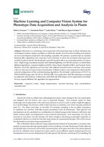
receives observations ot,n (s) at time t from n sensors with some certainty, given by conditional probability pn (o | s). A reward function R incentivize an agent to reach the desired destination, while it can be additionally engineered to ensure certain agent behavior, like obstacle avoidance, curiosity for exploration, maximizing speed, etc. A policy is approximated with a deep neural network, using observations ot,n (s) as inputs. A simplest class of navigation is obstacle avoidance, where agent’s goal is to move within a scene while avoiding collisions with obstacles. In [30] authors propose a reinforcement learning approach to this problem as opposed to conventional mapping and planning algorithms. The architecture is comprised of two neural networks (Fig. 1a). At first visual observations are inputted to a fully convolutional neural network [31], predicting depth from RGB observations. Second, network, trained with DoubleDQN [32] algorithm solves obstacle avoidance task in simulated environments. Actions are defined in discretized form to control linear and angular velocities. Reward function r = v · cos(ω) · δt, where v and ω are local linear and angular velocities respectively and δt is the time of each training loop, is engineered to incentivize the robot to move as fast as possible and to penalize if rotating on the spot. In case of a collision the agent is imposed an additional penalty of −10 and the episode is terminated. An episode is terminated with no additional penalty after 500 steps, hence robot is required to move within a scene as long as possible. π (a|s, g) π (a|s)
POLICY
π (a|s, g) rt1
POLICY
rt1
POLICY
rt1(g)
− CNN
CNN
ot(s)
x(g)
(a) Obstacle avoidance
CNN
ot(s)
(b) Image-based
RNN
x(g)
CNN
ot(s)
(c) Language-based
Fig. 1: Examples of navigation architectures The described setup allows an agent to successfully navigate within a scene, while avoiding obstacles, but not to reach a certain destination. To achieve that reward function may be engineered to reward an agent if it decreases the distance to a destination or to a set of landmarks [33] on each step. While a lot of reinforcement learning problems, including 2D and 3D mazes, are solved in a such a way, this setup is inflexible. In this case, the goal gets hardcoded in the weights θ of deep neural network approximating parametrized policy πθ (a | s). Therefore goal change requires re-training of the model. To avoid this one can additionally condition a policy on g: πθ (a | s, g) where g is the goal or a target to navigate a robot, hence reformulating navigation
problem being target-driven. A target can be set with explicit location coordinates, distances to landmarks [33], or given an image of destination [34], image of object to locate within a scene, or an instruction in natural language [29, 35], thus learning a mapping from a 2D image or a sequence in natural language to a policy. In [34] authors train an agent to navigate to new targets without re-training, specifying the navigation destination as inputs to the model, instead of hardcoding the target in model reward function. Both observations at each time step ot (s) and the target image x(g) are given by the agent’s RGB camera serve as inputs to convolutional siamese network [36]. It consists of two identical twin networks with shared parameters that transform inputs to the same embedding space and then fuse them using absolute difference. The obtained representation which can be viewed as a notion of similarity of an observation and a goal is then inputted to the scene-specific policy network (Fig. 1b). A reward is constructed giving a goal-reaching reward of 10 and small penalty (−0.01) on each step is imposed to encourage shorter navigation trajectories. In language-based visual navigation agent given natural language instruction x(g) = {x1 , . . . , xn } is expected to navigate to a goal position g. The agent’s action set A consists of linear and angular movement actions and a special action stop ending an episode. Language instruction x(g) and visual observations ot (s) at each time step are encoded with recurrent and convolutional neural networks respectively and inputted to a policy network, approximating policy πθ (a | s, g) (Fig. 1c). A reward is given in terms of the final navigation error, which is the distance to the targets position [35]. Challenges Solving visual navigation problem with reinforcement learning are effective in environments of ever-increasing complexity [37] – simple mazes, 3D games [38], photorealistic simulated environments [39, 24], city maps [33] and real environments [30]. Nevertheless, reinforcement learning for robot navigation faces a number of challenges. Reinforcement learning has low sample efficiency, learning by trial-and-error with high-dimensional state and action spaces guided only with reward provided by the environment requires millions of episodes. Often the rewards are sparse, in extreme case being an indication whether an agent has succeded or failed to reach the desired goal. Moreover training a real robot to navigate in the physical world pose additional challenges, being inefficient in terms of costs, time, risk of self-damage, property damage or even be a harm to humans. Usually, real environments are partially observable, thus an agent does not have a perfect knowledge of the state, receiving observations from sensors from which state can be only estimated. A robot must operate in the environments on large horizons, augmenting perception with reasoning. Reinforcement learning benefits from recent success in deep learning. Nowadays, representation learning of high-dimensional visual inputs and policy approximation are largely addressed with deep neural networks. Generally, to deal with low sample efficiency, learning is moved to simulations and pre-trained models further are fine-tuned on real environments. To improve statistical effi-
ciency various techniques to carefully re-use experience pool are developed, with hindsight experience replay [40] allowing an agent to learn from failures being a great example. Reward engineering may shorten effective problem horizon by introducing immediate rewards. In many cases sparse binary rewards can be reformulated to more dense ones, as an example instead of a binary reward for reaching a destination one can reward an agent on each step if the agent decreases the distance to it. Another approach is to augment loss with auxiliary tasks, as predicting visual modality from raw RGB data, loop closures [37], intersections or line crossings [41], providing more dense reward signals. An agent, able to reason how to tackle long-term dependencies should possess memory at different timescales. Augmenting policy networks with external memory shown increased agent’ abilities to navigate, extrapolating knowledge to unseen environments. We will describe simulators, knowledge transfer and memory-augmented architectures in more detail. Simulators and transfer learning Until recently visual data generated with simulators was not realistic-looking [42], so a virtual-to-real model transfer is highly desirable. The latest generation of simulators [39, 41, 24, 43] aims to narrow the gap between real and virtual world and offers realistic-looking visual data in different modalities. Besides RGB data most simulators do provide depth, normals, object and semantic segmentation. In this environments, agents can be equipped with different numbers of cameras, able to simulate different setups, including monocular and stereo ones. Simulators can leverage existing open-source 3D synthetic [44] or real [45] datasets or using proprietary 3D scenes [41, 24, 43], be either multi-purpose or dedicated to specific scenarios like autonomous driving [41] or UAV navigation [43]. Transfer learning involves a transfer of knowledge of a model trained on a source domain A to a transfer domain B. In case of reinforcement learning for visual robot navigation this includes transferring knowledge from a domain of simulated visual observations generated by a simulator to a domain of realworld visual sensor inputs. Another task is transferring knowledge between old and new domains of actions, i.e. leveraging prior knowledge to perform different navigational tasks and learning to navigate in unseen environments. There are a number of transfer learning strategies exist. Domain randomization [46, 47], while being conceptually simple, comes with insight that if a model was trained on a large number of simulated environments, and have seen enough variations in data, with different textures, lighting conditions, occlusions and scene dynamics, even it is not realistic, it would be able to generalize to perform well on real data [47, 30]. For navigation tasks this involves randomization of actions allowing an agent to over-explore the state-action space, thus further being applied to the desired task the agent is capable to use knowledge from a larger experience pool. In domain adaptation, a model pre-trained on synthetic data, either RGB input, depth or semantic segmentation, is then fine-tuned on real data, allowing
to learn on a smaller amount of real data. This approach is a mainstream, being a successful strategy in a variety of tasks [48]. As an alternative [49, 50] proposed to sidestep it by converting non-realistic virtual image input from a simulator into realistic one using image-to-image translation model, which takes synthetic image generated by a simulator and outputs realistic image, using semantic segmentation as interim representation, thus allowing to simplify or even abandon further fine-tuning. External memory A self-navigating robot should possess intelligent behavior, equipped both with perception and reasoning. It should be capable of handling long-term spatio-temporal dependencies, which is not the case for feedforward architecture of a policy network which is inherently reactive. Recurrent neural networks architectures such that LSTM [51] improve agent capabilities to reason, but have a set of disadvantages. Memory is tied up in the activations of the latent state of the networks, hence to increase the amount of memory one needs to increase the size of the network and therefore its’ computational cost. On the other side, memory tends to be fragile, due to residing in the space of the activations, that are being constantly updated [52]. π
π
π
POLICY
POLICY
POLICY
DNC CONTROLLER
CNN
CNN
CNN
ot(s)
(a) Feedforward
ot(s)
(b) LSTM
MEMORY MATRIX
ot(s)
(c) Memory-augmented network
Fig. 2: Policy networks Memory-augmented neural networks [53, 54] with Differetiable Neural Computer [52] being the most prominent one notably improve handling long-term dependencies. DNC architecture (Fig. 2c) allows features to be stored in the external memory matrix, by imposing learnable read and write operations. Information retrieval can be performed by content similarity or in a sequential manner. A policy network augmented with external memory have shown to solve navigation problems in environments with dead-end obstacles [55], which pose difficulties for simpler LSTM policy networks (Fig. 2b). Other than general external memory, a large body of work is devoted to specific neural memory architectures for RL-based visual navigation, powering agents with abilities to explicitly memorize map [56, 57] of the environment, and further localize [58] and plan [59], thus reiterating classical ideas within the reinforcement learning framework.
4
Conclusions
We briefly reviewed the RL technology. We provided a short overview of modern applications of reinforcement learning to computer vision and robot navigation tasks.
Acknowledgement The work was supported by the Skoltech NGP Program No. 1-NGP-1567 “Simulation and Transfer Learning for Deep 3D Geometric Data Analysis” (a SkoltechMIT joint project).
References 1. F. Bonin-Font, A. Ortiz, and G. Oliver. Visual navigation for mobile robots: A survey. Journal of Intelligent and Robotic Systems, 53(3):263–296, 2008. 2. A.P. Kuleshov, A.V. Bernstein, and E.V. Burnaev. Mobile robot localization via machine learning. In Lecture Notes in Computer Science, pages 276–290. Springer, 2017. 3. A. Kuleshov, A. Bernstein, E. Burnaev, and Yu. Yanovich. Machine learning in appearance-based robot self-localization. In IEEE Conference Publications, editor, 16th IEEE International Conference on Machine Learning and Applications (ICMLA), 2017. 4. R. Sutton and A. Barto. Reinforcement Learning: an Introduction. MIT Press, Cambridge, Mass, 1998. 5. L. P. Kaelbling, M. L. Littman, and A. P. Moore. Reinforcement learning: A survey. Journal of Artificial Intelligence Research, 4:237–285, 1996. 6. E. Burnaev and M. Panov. Adaptive design of experiments based on gaussian processes. In A. Gammerman et. al., editor, Lecture Notes in Artificial Intelligence. Proceedings of SLDS-2015, pages 116–126. 2015. 7. E. Burnaev, I. Panin, and B. Sudret. Effecient Design of Experiments for Sensitivity Analysis based on Polynomial Chaos Expansions. Ann. Math. Artif. Intell, 2017. 8. M. L. Puterman. Markovian Decision Processes - Discrete Stochastic Dynamic Programming. John Wiley & Sons Inc., New York, 1994. 9. R. Bellman. Dynamic Programming. Princeton University Press, Princeton, NJ, 1957. 10. C. J. C. H. Watkins and P. Dayan. Q-learning. Machine Learning, 8(3):279–292, 1992. 11. T. Jaakola, M. Jordan, and S. Singh. On the convergence of stochastic iterative dynamic programming algorithms. Neural Computation, 6(6):1185–1201, 1994. 12. Ronald J. Williams. Simple statistical gradient-following algorithms for connectionist reinforcement learning. Mach. Learn, 8(3-4):1992, May 1992. 13. Y. LeCun, Y. Bengio, and G. Hinton. Deep learning. Nature, 521(7553):436–444, 2015. 14. E. V. Burnaev and P. D. Erofeev. The influence of parameter initialization on the training time and accuracy of a nonlinear regression model. Journal of Communications Technology and Electronics, 61(6):646–660, 2016.
15. E. V. Burnaev and P. V. Prikhod’ko. On a method for constructing ensembles of regression models. Automation and Remote Control, 74(10):1630–1644, 2013. 16. Y. Li. Deep reinforcement learning: An overview. in [cs.LG], pages 1–70, 2017. 17. J. R. Uijlings, K. E. Van De Sande, and et al. Selective search for object recognition. International journal of computer vision, 104(2):154–171, 2013. 18. P. Viola and M. Jones. Rapid object detection using a boosted cascade of simple features. In In Computer Vision and Pattern Recognition. CVPR 2001. Proceedings of the 2001 IEEE Computer Society Conference on (Vol. 1, pp. I-I). IEEE, 2001. 19. S. Ren, K. He, R. Girshick, and J. Sun. Faster r-cnn: Towards real-time object detection with region proposal networks. In Advances in neural information processing systems, pages 91–99, 2015. 20. J. C. Caicedo and S. Lazebnik. Active object localization with deep reinforcement learning. In 2015 IEEE International Conference on Computer Vision (ICCV), pages 2488–2496. IEEE, 2015. 21. Da Zhang, Hamid Maei, and et al. Deep reinforcement learning for visual object tracking in videos. preprint, arXiv, 2017. 22. W. Luo, P. Sun, Y. Mu, and W. Liu. End-to-end active object tracking via reinforcement learning. preprint, 2017. 23. Volodymyr Mnih, Adria Puigdomenech Badia, and et al. Asynchronous methods for deep reinforcement learning. In International Conference on Machine Learning, pages 1928–1937, 2016. 24. W. Qiu, F. Zhong, and et al. UnrealCV: Virtual Worlds for Computer Vision. ACM Multimedia Open Source Software Competition, 2017. 25. Jingjia Huang, Nannan Li, and et al. A Self-Adaptive Proposal Model for Temporal Action Detection based on Reinforcement Learning. 2017. 26. Serena Yeung, Olga Russakovsky, and et al. End-to-end learning of action detection from frame glimpses in videos. 10(1109):2678–2687, 2016. 27. Alessandro Giusti, Jerome Guzzi, and et al. A machine learning approach to visual perception of forest trails for mobile robots. IEEE Robotics and Automation Letters, 1:661–667, 2016. 28. A. I. Maqueda, A. Loquercio, and et al. Event-based Vision meets Deep Learning on Steering Prediction for Self-driving Cars. ArXiv e-prints, April 2018. 29. Peter Anderson, Qi Wu, and et al. Vision-and-language navigation: Interpreting visually-grounded navigation instructions in real environments. CoRR, abs/1711.07280, 2017. 30. Linhai Xie, Sen Wang, and et al. Towards monocular vision based obstacle avoidance through deep reinforcement learning. CoRR, abs/1706.09829, 2017. 31. Evan Shelhamer, Jonathan Long, and Trevor Darrell. Fully convolutional networks for semantic segmentation. 2015 IEEE Conference on Computer Vision and Pattern Recognition (CVPR), pages 3431–3440, 2015. 32. Hado van Hasselt, Arthur Guez, and David Silver. Deep reinforcement learning with double q-learning. In AAAI, 2016. 33. Piotr Mirowski, Matthew Koichi Grimes, and et al. Learning to navigate in cities without a map. arXiv preprint arXiv:1804.00168, 2018. 34. Yuke Zhu, Roozbeh Mottaghi, and et al. Target-driven visual navigation in indoor scenes using deep reinforcement learning. 2017 IEEE International Conference on Robotics and Automation (ICRA), pages 3357–3364, 2017. 35. X. Wang, W. Xiong, and et al. Look Before You Leap: Bridging Model-Free and Model-Based Reinforcement Learning for Planned-Ahead Vision-and-Language Navigation. ArXiv e-prints, March 2018.
36. Gregory Koch, Richard Zemel, and Ruslan Salakhutdinov. Siamese neural networks for one-shot image recognition. In ICML Deep Learning Workshop, volume 2, 2015. 37. Piotr W. Mirowski, Razvan Pascanu, and et al. Learning to navigate in complex environments. CoRR, abs/1611.03673, 2016. 38. M. Kempka, M. Wydmuch, and et al. ViZDoom: A Doom-based AI Research Platform for Visual Reinforcement Learning. ArXiv e-prints, May 2016. 39. Manolis Savva, Angel X Chang, and et al. Minos: Multimodal indoor simulator for navigation in complex environments. arXiv preprint arXiv:1712.03931, 2017. 40. Marcin Andrychowicz, Filip Wolski, and et al. Hindsight experience replay. In Advances in Neural Information Processing Systems, pages 5048–5058, 2017. 41. Alexey Dosovitskiy, German Ros, and et al. Carla: An open urban driving simulator. arXiv preprint arXiv:1711.03938, 2017. 42. Nathan P. Koenig and Andrew Howard. Design and use paradigms for gazebo, an open-source multi-robot simulator. 2004 IEEE/RSJ International Conference on Intelligent Robots and Systems (IROS), 3:2149–2154 vol.3, 2004. 43. Shital Shah, Debadeepta Dey, and et al. Airsim: High-fidelity visual and physical simulation for autonomous vehicles. In Field and Service Robotics, pages 621–635. Springer, 2018. 44. Shuran Song, Fisher Yu, and et al. Semantic scene completion from a single depth image. IEEE Conference on Computer Vision and Pattern Recognition, 2017. 45. Angel Chang, Angela Dai, and et al. Matterport3d: Learning from rgb-d data in indoor environments. arXiv preprint arXiv:1709.06158, 2017. 46. Josh Tobin, Rachel Fong, and et al. Domain randomization for transferring deep neural networks from simulation to the real world. 2017 IEEE/RSJ International Conference on Intelligent Robots and Systems (IROS), pages 23–30, 2017. 47. Fereshteh Sadeghi and Sergey Levine. Cad2rl: Real single-image flight without a single real image. CoRR, abs/1611.04201, 2017. 48. Jason Yosinski, Jeff Clune, and et al. How transferable are features in deep neural networks? In NIPS, 2014. 49. Yurong You, Xinlei Pan, Ziyan Wang, and Cewu Lu. Virtual to real reinforcement learning for autonomous driving. CoRR, abs/1704.03952, 2017. 50. Jingwei Zhang, Lei Tai, and et al. Vr goggles for robots: Real-to-sim domain adaptation for visual control. CoRR, abs/1802.00265, 2018. 51. Sepp Hochreiter and J¨ urgen Schmidhuber. Long short-term memory. Neural computation, 9 8:1735–80, 1997. 52. Alex Graves, Greg Wayne, and et al. Hybrid computing using a neural network with dynamic external memory. Nature, 538 7626:471–476, 2016. 53. Sainbayar Sukhbaatar, Arthur Szlam, and et al. End-to-end memory networks. In NIPS, 2015. 54. Alex Graves, Greg Wayne, and Ivo Danihelka. Neural turing machines. CoRR, abs/1410.5401, 2014. 55. Arbaaz Khan, Clark Zhang, and et al. Memory augmented control networks. In International Conference on Learning Representations, 2018. 56. Emilio Parisotto and Ruslan Salakhutdinov. Neural map: Structured memory for deep reinforcement learning. CoRR, abs/1702.08360, 2017. 57. Nikolay Savinov, Alexey Dosovitskiy, and Vladlen Koltun. Semi-parametric topological memory for navigation. arXiv preprint arXiv:1803.00653, 2018. 58. Devendra Singh Chaplot, Emilio Parisotto, and Ruslan Salakhutdinov. Active neural localization. CoRR, abs/1801.08214, 2018. 59. P´eter Karkus, David F. C. Hsu, and Wee Sun Lee. Qmdp-net: Deep learning for planning under partial observability. In NIPS, 2017.