the more traditional methods. To this end we used the data from a chocolate manufacturer, a toner cartridge manufacturer, as well as from the Statistics Canada ...
IGI PUBLISHING
ITJ3868
40 International of Avenue, IntelligentSuite Information Technologies, 3(4), 40-�7, 701 E. Journal Chocolate 200, Hershey PA 17033-1240, USAOctober-December 2007 Tel: 717/533-8845; Fax 717/533-8661; URL-http://www.igi-pub.com This paper appears in the publication, International Journal of Intelligent Information Technologies ,Volume 3, Issue 4 edited by Vijayan Sugumaran © 2007, IGI Global
Machine learning-Based Demand forecasting in supply chains Réal Carbonneau, Concordia University, Canada Rustam Vahidov, Concordia University, Canada Kevin Laframboise, Concordia University, Canada
ABstRAct Effective supply chain management is one of the key determinants of success of today’s businesses. However, communication patterns between participants that emerge in a supply chain tend to distort the original consumer’s demand and create high levels of noise. In this article, we compare the performance of new machine learning (ML)-based forecasting techniques with the more traditional methods. To this end we used the data from a chocolate manufacturer, a toner cartridge manufacturer, as well as from the Statistics Canada manufacturing survey. A representative set of traditional and ML-based forecasting techniques have been applied to the demand data and the accuracy of the methods was compared. As a group, based on ranking, the average performance of the ML techniques does not outperform the traditional approaches. However, using a support vector machine (SVM) that is trained on multiple demand series has produced the most accurate forecasts.
Keywords: new machine learning; supply chains; support vector machine (SVM)
IntRoDuctIon
A major facet of businesses today is the notion of supply chain integration, whereby resources are combined to provide value to the end consumer and where all the upstream firms realize the importance of integration. Such integration often relies heavily on, or at very least includes, sharing information
between various business partners (Zhao, Xie, & Wei, 2002). Although integration and sharing information can potentially reduce forecast errors, they are neither ubiquitous nor complete activities and forecast errors still abound. Collaborative forecasting and replenishment (CFAR) permits a firm and its supplier-firm to coordinate decisions
Copyright © 2007, IGI Global. Copying or distributing in print or electronic forms without written permission of IGI Global is prohibited.
International Journal of Intelligent Information Technologies, 3(4), 40-�7, October-December 2007 41
by exchanging complex decision-support models and strategies, thus facilitating integration of forecasting and production schedules (Raghunathan, 1999). The value of information sharing across the supply chain is widely recognized as the means of combating demand signal distortion (Lee, Padmanabhan, & Whang, 1997). However, there is a gap between the ideal of integrated supply chains and the reality (Gunasekaran & Ngai, 2004). Researchers have identified several factors that could hinder such long-term stable collaborative efforts. Premkumar (2000) lists some required critical issues that permit successful supply chain collaboration, including: (i) alignment of business interests, (ii) long-term relationship management, (iii) reluctance to share information, (iv) complexity of large-scale supply chain management, (v) competence of personnel supporting supply chain management, and (vi) performance measurement and incentive systems to support supply chain management. In many supply chains there are power regimes and power sub-regimes that can prevent supply chain optimization (Cox, Sanderson, & Watson, 2001). The introduction of inaccurate information into the system could also lead to demand distortion, for example, double forecasting and ration gaming by the partners, ordering more quantities than needed despite the presence of a collaborative system and an incentive towards its usage (Heikkila, 2002). The over-emphasis on investing in extensive relationships among the partners could lead to a “lock-in” situation, thus seriously jeopardizing the flexibility of the supply chain (Gossain, Malhotra, & El Sawy, 2005; White, Daniel, & Mohdzain, 2005). Gossain et al.(2005) have recently argued that developing robust and reconfigurable links would promote the agility of
the chain in terms of offering and partnering flexibilities (Gossain et al., 2005). In their study they have found that while the quality of information sharing in a supply chain could promote the flexibility, the breadth of information shared has a detrimental effect on it. The modularity and loose couplings between the partners have been identified as positive factors in this regard. White et al. have stressed the importance of emergent technologies in promoting agility in supply chains (White et al., 2005). In light of the these considerations, the problem of forecasting distorted demand is of significant importance to businesses, especially those operating towards the upstream end of the extended supply chain. The purpose of this work is to investigate the potential value of applying advanced machine learning techniques, including artificial neural networks (ANN), recurrent neural networks (RNN), and support vector machines (SVM) to demand forecasting in supply chains. The performance of these machine-learning (ML) methods is compared against baseline traditional approaches, such as exponential smoothing, moving average, linear regression, and the Theta model. To this end we have collected the real industry data from three different sources. The first two data sets are from the enterprise systems of a chocolate manufacturer and a toner cartridge manufacturer. Both of these companies, by the nature of their position in the supply chain, are subject to considerable demand distortion. The third source of data comes from the Statistics Canada manufacturing survey. Inclusion of this survey in the study has the aim of increasing the validity and facilitating the possibility of replication of results by others.
Copyright © 2007, IGI Global. Copying or distributing in print or electronic forms without written permission of IGI Global is prohibited.
42 International Journal of Intelligent Information Technologies, 3(4), 40-�7, October-December 2007
BAckgRounD Demand Distortion in supply chains
One of the major purposes of supply chain collaboration is improving the accuracy of forecasts (Raghunathan, 1999). Since full collaboration is not always possible, it is important to investigate the feasibility of forecasting demand in the absence of extensive information from other partners. The source of the demand distortion in the extended supply chain simulation is due to demand signal processing by the members in the supply chain (Forrester, 1961). According to Lee et al. (1997), demand signal processing means that each party in the supply chain does some processing on the demand signal, thus transforming it before passing it along to the next member. As the end-customer’s demand signal moves up the supply chain, it becomes increasingly distorted. This occurs even if the demand signal processing function is identical in all parties of the extended supply chain. For example, even if all supply chain members use a six-month trend to forecast demand, distortion will still occur. It has been shown that the use of simple techniques, such as moving average, naïve forecasting, or demand signal processing will induce the bullwhip effect (Dejonckheere, Disney, Lambrecht, et al.,2003), while autoregressive linear forecasting could diminish it (Chandra & Grabis, 2005). Furthermore, a simulation based study has shown that genetic algorithmbased artificial agents can achieve lower overall costs in managing supply chain than human players can (Kimbrough, Wu, & Zhong, 2002).
traditional forecasting techniques
Extensive research on forecasting has provided a large number of forecasting techniques and algorithms in mathematics, statistics, operations management, and supply chain academic outlets. Forecasting competitions have consistently found that the simpler forecasting methods had better overall accuracy than more complex ones (Makridakis, Andersen, Carbone, et al., 1982; Makridakis, Chatfield, Hibon et al., 1993; Makridakis & Hibon, 1979; Makridakis & Hibon, 2000). The M3-competition included academic and commercial forecasting methods, including Naïve/simple, explicit trend models, decomposition, variations of the general ARMA (autoregressive moving average) model, expert systems, and neural networks. The results, even with a new and much enlarged set of data demonstrated, once more, that simple methods developed by practicing forecasters do as well, or in many cases better, than more sophisticated ones (Makridakis & Hibon, 2000).
Machine learning techniques
As the number of forecasting techniques and parameters increase, it becomes more difficult to choose the appropriate one in a particular context. One possible solution is to rely on a class of algorithms called “universal approximators,” which can approximate any function to an arbitrary accuracy. Using such universal approximators, any required function between past and future data can be learned, thus effectively making other forecasting techniques a subset of the functions that the universal approximators can learn. ML techniques, such as artificial neural networks and support vector ma-
Copyright © 2007, IGI Global. Copying or distributing in print or electronic forms without written permission of IGI Global is prohibited.
International Journal of Intelligent Information Technologies, 3(4), 40-�7, October-December 2007 43
chines are universal approximators and can be used to learn any function. Forecasting time series, such as those in supply chains, involves a data domain that is highly noisy. It is highly desirable only to learn true patterns in the data that will be repeated in the future and to ignore the noise. The ML-based techniques have two important features that are useful for supply chain forecasting problems in the presence of noise: (i) the ability to learn an arbitrary function; and (ii) the ability to control the learning process itself. ANN and RNN are frequently used to predict time series data (Dorffner, 1996; Giles, Lawrence, & Tsoi, 2001; Herbrich, Keilbach, Graepel et al., 1999; Landt, 1997). For example, because manufacturer’s demand is considered a chaotic time series, RNNs perform backpropagation of error through time that permits the neural network to learn patterns through to an arbitrary depth in time. SVM, a more recent learning algorithm that has been developed from statistical learning theory (Vapnik, 1995; Vapnik, Golowich, & Smola, 1997), have a very strong mathematical foundation and have been previously applied to time series analysis (Mukherjee, Osuna, & Girosi, 1997).
REsEARch MEthoDology
This work addresses the question: Do MLbased forecasting techniques provide more accurate forecasts of distorted customer demand in a supply chain as experienced by the manufacturer? In essence, we set out to investigate whether ML, in general, performs better than traditional forecasting techniques. To this end, we conducted experiments to compare the accuracy of ML forecasting techniques with traditional ones in the context of noisy supply chain. In our study the traditional forecasting
techniques were represented by moving average, trend, exponential smoothing, and multiple linear regression. Additionally, based on the M3-competition (Makridakis & Hibon, 2000), we included the Theta method (Assimakopoulos & Nikolpoulos, 2000), which exhibited impressive results. For completeness, we also included the frequently used, classic ARMA, sometimes also referred to as the Box-Jenkins model (Box, Jenkins, & Reinsel, 1994). The MLbased forecasting techniques were ANN, RNN, and SVM.
Data sources
We have included data from manufacturers that have integrated ERP systems, where every product or service that goes in and out of the system is controlled, as are all monetary transactions. There are two manufacturers who provided demand data as extracted from their ERP systems. The first manufacturer produces chocolate starting from the cocoa beans, which must be roasted, converted into cacao, and then combined with other ingredients according to recipe. The geographic scope of the data set is North America. Since the inception of the ERP system and up to the time of the extraction of the data for this research, information was available for 47 months (October 2000-November 2003) of demand for a product. We considered the top 100 products with the most cumulative volume during this period since these are the most important products for which the accuracy of forecasts is critical. The second manufacturer specializes in generic photocopier and laser printer toner cartridges and other related products. The geographic scope of the data is North America. The demand data extracted from the ERP system represents a total of 65
Copyright © 2007, IGI Global. Copying or distributing in print or electronic forms without written permission of IGI Global is prohibited.
44 International Journal of Intelligent Information Technologies, 3(4), 40-�7, October-December 2007
periods of data. Again only the top 100 products were retained for the experiment since they are considered most important. The total number of active products in their system being 3,369, the 100 products represented less than three percent of all products. However, these top products account for 38.35 percent of sales volume for the manufacturer. To add validity to the experiment, we included time series data about manufacturers demand as collected by Statistics Canada, that is, publicly available historical data that cover a large part of the manufacturing sectors in the Canadian economy. Specifically, the data source included the manufacturers’ monthly new orders by North American Industry Classification System (NAICS) referred to as table 304-0014 (Statistics Canada, 2005). This dataset provided a good way to experiment on a variety of demand patterns across a large number of industries (214 industrial categories.) We used most recent “new order” observations representing 12 years and four months of data or 148 periods. To be consistent with the other two datasets we randomly selected 100 categories. The patterns in the Statistics Canada data are different from those of the individual manufacturers because of their aggregate nature and lengthy data collection time span. Variability is much lower than that of the individual manufacturers because of the aggregation effect.
ExpERIMEnts Data set preparation
We used a representative set of traditional forecasting techniques as a control group, and a set of machine learning techniques as a treatment group. To compare the two groups, every technique from each group
was used to forecast demand one month into the future for all of the 100 series for the three datasets previously identified. This resulted in a series of 4,700 forecast points for the chocolate manufacturer, 6,500 for the toner cartridge manufacturer and 14,800 for the Statistics Canada dataset for every technique tested. However, since all forecasting techniques require past data to make a forecast into the future, there was a predetermined startup period that slightly reduced the number of forecast observations. Additionally, the demand time series was formally separated into a training set and testing set. This is particularly important for the ML techniques, where the training set was used for ML models to learn the demand patterns and the testing set used to estimate how well the forecasting capability could generalize in the future. The main performance measure used was the absolute error (AE) measure for every forecast data point. This resulted in a series of absolute error values for a specified forecasting technique. To make the absolute error comparable across products, we normalized this measure by dividing it by the standard deviation of the training set. Thus, the performance of different techniques was compared in terms of normalized absolute error (NAE). We used 80 percent of the time series data for training and 20 percent of the data for testing. We then employed all of the selected techniques to produce forecasts using MATLAB 7.0 environment (MathWorks, 2005b).
Models
The ARMA model combines both autoregressive forecast and a moving average forecast. To minimize the error, we optimized the lag used in the auto-regression
Copyright © 2007, IGI Global. Copying or distributing in print or electronic forms without written permission of IGI Global is prohibited.
International Journal of Intelligent Information Technologies, 3(4), 40-�7, October-December 2007 4�
portion and the lag used in the moving average portion. This functionality is provided by the MATLAB GARCH Toolbox (MathWorks, 2005a). The Theta model in our implementation mimicked the one used in M3 forecasting competition. First, the linear trend was calculated, and then the exponential smoothing performed on double of the difference between the raw data and trend values to minimize the error on the training set. The two individual series, the linear trend and the optimized exponential smoothing on the decomposed series were recombined by an average of the two. We implemented two versions of the Theta, one with the initial value chosen for the initialization and the other with the average of the training set as the initialization.
transfer function is represented by ( ), and the linear transfer function is represented by ( ). All of the inputs to the neural network, as well as the output are individually scaled between -1 and 1 to ensure that they are within the appropriate range for neural network training. The final results are then unscaled to permit comprehensible analysis and usage. The first implementation of neural networks is based on the traditional back propagation algorithm. An adaptive variable learning rate training algorithm has been adopted, which adjusts the learning rate for the current learning error space (Hagan, Demuth, & Beale, 1996). This algorithm tries to maximize the learning rate subject to stable learning, thus adapting to the complexity of the local learning error space. In addition to the variable learning rate, our first neural network learning algorithm also includes the momentum (Hagan, Demuth, & Beale, 1996). To help the neural network stop training before it overfits the training set to the detriment of
Neural Networks
The relevant aspects of the supply chain demand modeling neural network are displayed in Figure 1. In this figure, the sum is represented sigma (Σ), the tan-sigmoid
Figure 1. Supply chain demand modeling neural network design Outputs
Neuron 1
Output Layer
Hidden Layer 1
w1 w2
Weights
Weights
Input1
w1 Bias
Neuron 2
Input2
w (n*h)+ h
...
...
Inputi
Bias
Neuron h
Bias
w3
...
Neuron 3
Input3
w2 Neuron 1
Bias
...
Current and Past Demand Window
Inputs
Supply Chain Demand Modeling Neural Network Design
Future Demand
Bias
w (h*o)+ o Legend: h = Hidden Layer Neurons i = Inputs o = Outputs w = Weights
Copyright © 2007, IGI Global. Copying or distributing in print or electronic forms without written permission of IGI Global is prohibited.
4� International Journal of Intelligent Information Technologies, 3(4), 40-�7, October-December 2007
generalization, we use a cross-validation set for early stopping. This cross-validation set is an attempt to estimate the neural network’s generalization performance. We have defined the cross-validation set as the last 20 percent of the training set. Additionally, we have also used the Levenberg-Marquardt algorithm (Marquardt, 1963) as applied to Neural Networks (Hagan, Demuth, & Beale, 1996; Hagan & Menhaj, 1994). This algorithm is one of the fastest training algorithms available with training being 10-100 times faster than simple gradient decent backpropagation of error (Hagan & Menhaj, 1994). The Levenberg-Marquardt neural networktraining algorithm is further combined into a framework that permits estimation of the network’s generalization by the use of a regularization parameter. This regularization parameter permits the control of the ratio of impact between reducing
the error of the network and the number of weights, or power of the network so that one can be less concerned with the size of the neural network and control its effective power directly. The tuning of this regularization parameter is automated within the Bayesian framework (MacKay, 1992) and, when combined with the Levenberg-Marquardt training algorithm, results in high performance training combined with a preservation of generalization by avoiding overfitting of the training data (Foresee & Hagan, 1997). An example of a Levenberg-Marquardt with automated Bayesian regularization training session is presented in Figure 2 where we can see that the algorithm is attempting to converge the network to a point of best generalization based on the current training set. Even though this particular network has 256 weights, the algorithm is controlling the power of the neural network at effective
Figure 2. Example Levenberg-Marquardt neural network training details.
Copyright © 2007, IGI Global. Copying or distributing in print or electronic forms without written permission of IGI Global is prohibited.
International Journal of Intelligent Information Technologies, 3(4), 40-�7, October-December 2007 47
number of parameters of about 44. The network could further reduce the error on the training set (Sum of Squared Error: SSE) since it could use all 256 weights. However, it has determined that using more than the 44 weights will cause overfitting of the data and thus, the reduced generalization performance. Compared to the early stopping based on a cross validation set, the LevenbergMarquardt with automated Bayesian regularization training algorithm is superior especially for small datasets since separating out a cross validation set it not required because the algorithms looks at all of the training data.
Recurrent Neural Networks
The recurrent neural network architecture is the same as the described feedforward architecture, except for one essential difference. There are recurrent network connections within the hidden layer as presented in the subset architecture in Figure 3. This architecture is known as an Elman network
(Elman, 1990). The recurrent connections feed information from the past execution cycle back into the network. This permits a neural network to learn patterns through time. In our experiments we used the two previously described training methods, the variable learning rate with momentum and early stopping based on cross validation set error and the Levenberg-Marquardt with automated Bayesian regularization training algorithm.
Support Vector Machine
The support vector machine software implementation selected for the current experiment was mySVM (Rüping, 2005), which is based on the SVMLight optimization algorithm (Joachims, 1999). The inner product kernel was used and the complexity constant was automatically determined using cross-validation procedure. Two cross-validation procedures were tested. The first one was a simple 10 fold cross validation that ignores the time direction of the data. Thus, for 10 iterations, 9/10th
Figure 3. Recurrent subset of neural network design
rw 1 rw 2
Hidden Layer 1
Weights
Recurrent Subset of Supply Chain Demand Modeling Neural Network Design
Neuron 1
Bias
Neuron 2
...
Legend: h = Hidden Layer Neurons rw = Recurrent Weights
Bias
Neuron 3
...
Bias
Neuron h
rw (h*h)
Bias
Copyright © 2007, IGI Global. Copying or distributing in print or electronic forms without written permission of IGI Global is prohibited.
4� International Journal of Intelligent Information Technologies, 3(4), 40-�7, October-December 2007
of the data were used to build a model and the remaining 1/10th was used to test the accuracy. The second one simulated time ordered predictions, called windowed cross validation. This cross validation procedure split the training data set into 10 parts and the algorithm trained the model using 5 parts and tested on a 6th part. This 5-part window was moved along the data, which resulted in the procedure being repeated 5 times. For example blocks 1-5 were used to train and the model was tested on block 6, then blocks 2-6 were used to train the model and tested on block 7, and so on. The errors of these five models were averaged and the complexity constant with the smallest cross validation error was selected as the level of complexity that provided the best generalization. Increasing the complexity constant form a very small value (low computational power) to a very large value (overfitting the data) results in an error curve, which permits the minimization of the generalization error. An example error
curve for the complexity constant search on a 10-fold cross validation set with a five-fold sliding window for the complexity constant range between 0.00000001 and 100 with a multiplicative step of 1.1, is presented in Figure 4. The complexity constant of 0.0122 provides a forecast that represents the level of patterns learning that seems to generalize best.
Super Wide Models
Since the available time series are somewhat short, there may not be sufficient examples for learning complex patterns. The separation of the data set into training, cross-validation and testing sets, and the loss of periods due to the windowing all combined to further reduce the set of usable observations. Based on the assumption that several products of the same manufacturer probably have similar demand patterns, we introduced what we called a super wide model. This method takes a wide selection of time series from the same problem
Figure 4. SVM cross validation error for complexity constant
Copyright © 2007, IGI Global. Copying or distributing in print or electronic forms without written permission of IGI Global is prohibited.
International Journal of Intelligent Information Technologies, 3(4), 40-�7, October-December 2007 4�
domain and combines them into one large model that effectively increases the number of training examples. This large number of training examples permits an increase in input dimensionality (e.g., larger window size) and model complexity. For example, in this experiment, we consider 100 time series for each of the sources. With the super wide model, we use the data from all of the 100 time series simultaneously to train the model. This provides a large number of training examples and permits us to greatly increase the window size so that the models can look deep into the past data. For example, for the chocolate factory data set, there are 100 products and 47 periods of time series data. Once the training and testing set are separated, we have 38 periods of data. For this type of model, we choose a window size of 50 percent, which is a perfect balance between modeling the demand behavior as a function of the past 50 percent of the data and using 50 percent of the data as examples. Using this large window size of 50 percent with the traditional time series model would provide a training set of 19 examples for a window size of 19 that would not represent very much data to identify patterns. However, with the super wide model, we would end up with 1,900 examples for a window size of 19, which represent sufficient data to find the complex patterns for the problem domain. All of the models that learn from past demand, such as the multiple linear regression, neural networks, and support vector machines will be tested also on the super wide data, with the only exception recurrent neural networks. Although training a recurrent neural network on a super wide model is feasible in principle, it would require a reset of the recurrent connections for every product because time lagged signals between products would not make
sense. The neural network models were enlarged to 10 hidden layer neurons, which in combination with the very large window provide a large input space, resulting in large network sizes compared to the patterns that were to be expected.
REsults
This section discusses the performance of the selected models on three data sets. Table 1 presents the MAE of all the tested forecasting techniques as applied to the chocolate manufacturer’s dataset in ascending order of error with the best-performing techniques at the top of the list, and the worst ones at the bottom. The results are also provided in similar format for the toner cartridge manufacturer’s dataset (Table 2) and the Statistics Canada manufacturing dataset (Table 3). From these results we can see that one of the ML approaches, the SVM under the super wide modeling approach is at the top of all three data sets by providing consistently better performance. If we ignore the super wide models, we find that the results of previous research and the very large M3 competition were essentially reproduced, that is, simple techniques outperform the more complicated and sophisticated approaches. For example, in the two primary datasets of interests, the chocolate and the toner cartridge manufacturer, exponential smoothing had the best performance. Noticeably, the toner cartridge data set was so noisy or the patterns changed so much with time that even the exponential smoothing with a fixed parameter of 20 percent outperformed (Table 2—Rank 3) the automated one (Table 2—Rank 5), which optimized the parameter for the training set. Essentially this indicates that the automated exponential smoothing overfits the data, which is somewhat surprising.
Copyright © 2007, IGI Global. Copying or distributing in print or electronic forms without written permission of IGI Global is prohibited.
�0 International Journal of Intelligent Information Technologies, 3(4), 40-�7, October-December 2007
Table 1. Performance of forecasting techniques for chocolate manufacturer’s dataset Rank
Method
Group
NMAE
1
SuperWide Support Vector Machine, Windowed Cross Validation
Treatment
0.7693
2
SuperWide Support Vector Machine, Cross Validation
Treatment
0.7717
3
SuperWide Multiple Linear Regression
Control
0.7776
4
SuperWide Neural Network, Cross Validation
Treatment
0.7998
5
Exponential Smoothing, Automatic, Initialization=First
Control
0.8270
6
Exponential Smoothing, 20 percent
Control
0.8329
7
Theta, Exponential Smoothing Initialization=First
Control
0.8347
8
Moving Average, 6 Periods
Control
0.8381
9
Moving Average, Automatic
Control
0.8534
10
Exponential Smoothing, Automatic, Initialization=Average
Control
0.8613
11
Theta, Exponential Smoothing Initialization=Average
Control
0.8775
12
Multiple Linear Regression
Control
0.9047
13
SuperWide Neural Network, Levenberg-Marquardt, Bayesian Regularization
Treatment
0.9209
14
Recurrent Neural Network, Levenberg-Marquardt, Bayesian Regularization
Treatment
0.9307
15
Neural Network, Levenberg-Marquardt, Bayesian Regularization
Treatment
0.9331
16
Support Vector Machine, Cross Validation
Treatment
0.9335
17
Support Vector Machine, Windowed Cross Validation
Treatment
0.9427
18
Neural Network, Back-Propagation, Cross Validation
Treatment
0.9810
19
Recurrent Neural Network, Back-Propagation, Cross Validation
Treatment
0.9954
20
Auto Regressive Moving Average
Control
1.0151
21
Trend, Automatic
Control
1.6043
22
Trend, 6 Periods
Control
8.1978
Table 2. Performance of forecasting techniques for toner cartridge manufacturer’s dataset Rank
Method
Group
NMAE
1
SuperWide Support Vector Machine, Cross Validation
Treatment
0.6777
2
SuperWide Support Vector Machine, Windowed Cross Validation
Treatment
0.6781
3
Exponential Smoothing, 20%
Control
0.6928
4
Moving Average, 6 Periods
Control
0.6993
5
Exponential Smoothing, Automatic, Initialization=First
Control
0.6994
6
Support Vector Machine, Windowed Cross Validation
Treatment
0.7003
7
Moving Average, Automatic
Control
0.7054
8
SuperWide Multiple Linear Regression
Control
0.7060
9
Support Vector Machine, Cross Validation
Treatment
0.7221
10
Theta, Exponential Smoothing Initialization=First
Control
0.7244
continued on following page Copyright © 2007, IGI Global. Copying or distributing in print or electronic forms without written permission of IGI Global is prohibited.
International Journal of Intelligent Information Technologies, 3(4), 40-�7, October-December 2007 �1
Table 2. continued 11
Exponential Smoothing, Automatic, Initialization=Average
Control
0.7259
12
Theta, Exponential Smoothing Initialization=Average
Control
0.7358
13
Multiple Linear Regression
Control
0.7677
14
SuperWide Neural Network, Levenberg-Marquardt, Bayesian Regularization
Treatment
0.7781
15
Recurrent Neural Network, Back-Propagation, Cross Validation
Treatment
0.8090
16
Recurrent Neural Network, Levenberg-Marquardt, Bayesian Regularization
Treatment
0.8187
17
Neural Network, Levenberg-Marquardt, Bayesian Regularization
Treatment
0.8189
18
Neural Network, Back-Propagation, Cross Validation
Treatment
0.8498
19
SuperWide Neural Network, Cross Validation
Treatment
0.8818
20
Auto Regressive Moving Average
Control
0.9319
21
Trend, Automatic
Control
1.6058
22
Trend, 6 Periods
Control
8.6140
Table 3. Performance of forecasting techniques for statistics Canada manufacturing dataset Rank
Method
Group
NMAE
1
SuperWide Support Vector Machine, Windowed Cross Validation
Treatment
0.4478
2
SuperWide Support Vector Machine, Cross Validation
Treatment
0.4547
3
Multiple Linear Regression
Control
0.4910
4
Support Vector Machine, Windowed Cross Validation
Treatment
0.4914
5
Support Vector Machine, Cross Validation
Treatment
0.4932
6
Theta, Exponential Smoothing Initialization=First
Control
0.5052
7
Exponential Smoothing, Automatic, Initialization=First
Control
0.5055
8
Exponential Smoothing, Automatic, Initialization=Average
Control
0.5086
9
Moving Average, Automatic
Control
0.5108
10
Theta, Exponential Smoothing Initialization=Average
Control
0.5137
11
SuperWide Multiple Linear Regression
Control
0.5327
12
Moving Average, 6 Periods
Control
0.5354
13
Recurrent Neural Network, Levenberg-Marquardt, Bayesian Regularization
Treatment
0.5355
14
Neural Network, Levenberg-Marquardt, Bayesian Regularization
Treatment
0.5374
15
Exponential Smoothing, 20%
Control
0.5483
16
SuperWide Neural Network, Cross Validation
Treatment
0.5872
17
SuperWide Neural Network, Levenberg-Marquardt, Bayesian Regularization
Treatment
0.6453
18
Recurrent Neural Network, Back-Propagation, Cross Validation
Treatment
0.8060
19
Neural Network, Back-Propagation, Cross Validation
Treatment
0.8238
20
Auto Regressive Moving Average
Control
1.3662
21
Trend, Automatic
Control
1.9956
22
Trend, 6 Periods
Control
20.8977
Copyright © 2007, IGI Global. Copying or distributing in print or electronic forms without written permission of IGI Global is prohibited.
�2 International Journal of Intelligent Information Technologies, 3(4), 40-�7, October-December 2007
We arrive at the same conclusion with the moving average approach that was fixed to a window of 6 periods (Table 2—Rank 4). The automatic versions likewise had overfitting problems and had lower performance (Table 2—Rank 7) than setting a common parameter value (Table 2—Rank 4). The average error of the automatic exponential smoothing for the two manufacturer’s datasets was 0.7516; the average for the fixed exponential smoothing of 20 percent was 0.7501. The moving average with a window of 6 periods had an average error of 0.7561 and a mean difference significance of 0.2273 with the average of the automatic exponential smoothing. The average error of the automatic exponential smoothing for all three datasets was 0.6096; the average for the fixed exponential smoothing of 20 percent was 0.6337. The moving average with a window of six periods had an average error of 0.6288. Therefore, the automatic exponential smoothing, 20 percent exponential smoothing and the six period-window moving average all provided approximately the same performance. In case of the Statistics Canada dataset, the results were a little different; we found the MLR (Table 3 — Rank 3), SVM (Table 3—Ranks 4 and 5) and Theta (Table 3—Rank 6) outperformed exponential smoothing (Table 3—Rank 7). However, because these approaches had such poor performance on the chocolate and toner cartridge manufacturer datasets and that the performance gain by these over the ES method was very small, we did not consider these results relevant. They are most likely due to the very large amount of data (12 years) and the aggregate nature of the data that was less noisy. It is interesting to note that the trend approach (an informal way of planning by extrapolating that a certain trend will
continue in the future) was by far the worst forecasting approach since it always ranked at the bottom of all three tables. Also, ARMA and most of the ML approaches other than SVM showed a relatively poor performance. The overall best performance was obtained using SVMs in combination with the super wide data. Since we have previously identified that the best traditional technique was automatic exponential smoothing (it performed well on both manufacturers’ data, as well as the aggregate manufacturing data), we can calculate the forecast error reduction provided by the best ML approach. For the chocolate manufacturer’s dataset (Table 1—Rank 2 and 5), we found a 6.70 percent ((0.�270 - 0.7717) / 0.�270) reduction in the overall forecasting error and for the tone cartridge manufacturer dataset (Table 2—Ranks 1 and 5) we found a 3.11 percent ((0.���4 - 0.�777) / 0.���4) reduction in the overall forecasting error. In the case of the Statistics Canada manufacturing dataset (Table 3—Ranks 2 and 7), we found a 10.00 percent ((0.�0�� - 0.4�47 / 0.�0��) reduction in the forecasting error as compared to automatic exponential smoothing. This was an average of 4.90 percent for our two manufacturers’ dataset and an average of 6.61 percent for all three as compared to automatic exponential smoothing. The performance of the super wide models has a potential to improve further, if more products are included beyond the limit of 100 used in our research. We further examined the difference between the average error of traditional forecasting techniques and ML-based techniques. By taking the average error of the control and treatment group we can evaluate if ML in general presents a better solution. As noted earlier, the trend technique provided extremely poor forecasting and the
Copyright © 2007, IGI Global. Copying or distributing in print or electronic forms without written permission of IGI Global is prohibited.
International Journal of Intelligent Information Technologies, 3(4), 40-�7, October-December 2007 �3
error measurements produced were extreme outliers. However, they were not outliers in the sense of being a measurement error, they were correct values and were retained in the average calculation. Additionally, the trend forecasting techniques had to be retained in the experiment because it is representative of what practitioners use. According to Jain (2004), averages and simple trend are used 65 percent of the time. Using the results of the experiments on chocolate (Table 1) and toner cartridge manufacturer (Table 2), the average error in the control group was 1.5014 and the average error in the treatment group was 0.8356. It was not feasible to take all of the error points of the test sets for each forecasting technique and compare those of the control group with the treatment group since there would be 52,800 observations for the control group and 44,000 observations for the treatment group. However, considering the large difference between the averages and the large number of observations, we conclude that the treatment (ML) group had significantly outperformed the control (traditional) group. Accordingly, without any specific information on which traditional and ML techniques are best or if there is a lack of experience and knowledge related to traditional and ML techniques, one would be more likely to be better off in choosing a random ML solution to induce the lower expected error. We have also compared the best-performing ML vs. best-performing traditional technique. The difference between the SVM error average of 0.7154 and the automatic exponential smoothing error average of 0.7516 had a p-value of 0.0000. Across the three datasets the SVM error average was 0.5651 and the automatic exponential smoothing error average was 0.6096, a statistically significant difference with
p-value of 0.0000. Thus, we can conclude that the best ML approach has performed significantly better than the best traditional approach. Using the super wide data for the SVM modeling permitted an analysis of much more data simultaneously and thus produced a very high historical window size while still having a very large dataset to learn from. As a result of this, we set the historical window size to 50 percent of the history. However, we investigated whether 50 percent was the correct setting and whether this setting had an impact on the performance of the model. Although a historical window size of 50 percent seemed normal, we re-executed the super wide SVM models for a window size of 40 percent and one of 60 percent to evaluate the impact of this choice. The MAE for the super wide SVM with parameter optimization via standard cross-validation for a historical window size of 40 percent, 50 percent, and 60 percent are presented in Table 4. From these results we find that for the chocolate manufacturer’s dataset the error
Table 4. Sensitivity analysis of window size DataSet
Window MAE
Chocolate
0.40
0.7806
Chocolate
0.50
0.7717
Chocolate
0.60
0.7703
Toner Cartridge
0.40
0.6770
Toner Cartridge
0.50
0.6777
Toner Cartridge
0.60
0.6846
Statistics Canada
0.40
0.3903
Statistics Canada
0.50
0.4547
Statistics Canada
0.60
0.4414
Copyright © 2007, IGI Global. Copying or distributing in print or electronic forms without written permission of IGI Global is prohibited.
�4 International Journal of Intelligent Information Technologies, 3(4), 40-�7, October-December 2007
decreased when the window size increased, however, for the toner cartridge dataset the error increased with window size increase. The Statistics Canada manufacturing dataset showed mixed results with no trend. Thus, there is no evidence to indicate that a smaller or larger window size would have a significant impact on the performance. Thus, we found that the super wide SVM with parameter optimization via standard cross-validation was relatively insensitive to the window size and that a window size of 50 percent seemed to be an adequate choice.
conclusIon AnD DIscussIon
The purpose of this work has been to investigate the applicability and benefits of machine learning techniques in forecasting distorted demand signal with a high noise in the context of supply chains. Although there are several forecasting algorithms available to practitioners, there are very few objective and reproducible guidelines regarding which method should be employed. In this research, we have shown empirically that the best traditional method for a manufacturer is the automatic exponential smoothing with the first value of the series as the initial value. We have also found that all of the more advanced machine learning techniques have relatively poor performance, possibly due to the limited number of past time periods for any given product. None of the ML techniques can reliably outperform the best traditional counterpart (exponential smoothing) when learning and forecasting single time series. However, one important finding concerns the usefulness of combining the data about multiple products in what we called a super wide model in conjunction with a
relatively new technique, the support vector machine (SVM). The domain-specific empirical results show that this approach is superior to the exponential smoothing. The error reduction found range from 3.11 percent to 10 percent, which can result in large financial savings for a company depending on the cost related to inventory errors. This assuming that the company is already using the best forecasting method available, or otherwise the performance gains would be even greater. We feel confident with regards to the generalizability of our findings, since the work used actual data from a large number of products from two North American manufacturers, with the additional verification against Statistics Canada manufacturing survey. We also feel that as the number of products added to the combined time series model (super wide approach) increases, the performance could also increase. One important point to note is that SVM are computationally intensive and the cross validation based complexity parameter optimization procedure results in running a large amount of support vector machines depending on the precision of the complexity search. The longest running models in this research took over 3 days of processing on a modern computer. There are many optimization techniques that could be performed to reduce the processing time such as parallelization, which is trivial for a cross-validation procedure and reduction of the complexity term search precision. We hope that further optimizations to the SVM algorithms and the increase in processing power would reduce the processing time significantly. Once the models have been completed, they can be used for forecasting with relatively little processing time. There is also research into hardware based SVM implementations. One such project is the
Copyright © 2007, IGI Global. Copying or distributing in print or electronic forms without written permission of IGI Global is prohibited.
International Journal of Intelligent Information Technologies, 3(4), 40-�7, October-December 2007 ��
Kerneltron which provide performance increases by a factor of 100 to 10,000 (Genov & Cauwenberghs, 2001, 2003), thus increasing the probability that such large SVM applications are feasible in the medium term future. One important possibility for future research would be investigating the benefits of the ML techniques when using other sources of data and in the context of collaborative forecasting. This additional data may include economic indicators, market indicators, collaborative information sources, product group averages and other relevant information.
REfEREncEs Assimakopoulos, V., & Nikolpoulos, K. (2000). The theta model: A decomposition approach to forecasting. International Journal of Forecasting, 16(4), 521.
Dorffner, G. (1996). Neural networks for time series processing. Neural Network World, 96(4), 447-468. Elman, J. L. (1990). Finding structure in time. Cognitive Science, 14(2), 179-211. Foresee, F. D., & Hagan, M. T. (1997). GaussNewton approximation to Bayesian regularization. In Proceedings of the 1997 International Joint Conference on Neural Networks (pp. 1930-1935). Forrester, J. (1961). Industrial dynamics. Cambridge, MA: Productivity Press. Genov, R., & Cauwenberghs, G. (2001). Chargemode parallel architecture for matrix-vector multiplication. IEEE Trans. Circuits and Systems II: Analog and Digital Signal Processing, 48(10), 930-936. Genov, R., & Cauwenberghs, G. (2003). Kerneltron: Support vector “machine” in silicon. IEEE Transactions on Neural Networks, 14(5), 1426-1434.
Box, G., Jenkins, G. M., & Reinsel, G. (1994). Time series analysis: Forecasting and Giles, C. L., Lawrence, S., & Tsoi, A. C. (2001). Noisy time series prediction using recurrent control (3rd ed.). Englewood Cliffs, NJ: neural networks and grammatical inferPrentice Hall. ence. Machine Learning, 44, 161-184. Chandra, C., & Grabis, J. (2005). Application of multi-steps forecasting for restraining Gossain, S., Malhotra, A., & El Sawy, O. A. (2005). Coordinating for flexibility the bullwhip effect and improving invenin e-business supply chains. Jourmal of tory performance under autoregressive Management Information Systems, 21(3), demand. European Journal of Operational 7-45. Research, 166(2), 337. Cox, A., Sanderson, J., & Watson, G. (2001). Gunasekaran, A., & Ngai, E. W. T. (2004). Information systems in supply chain integration Supply chains and power regimes: Toward and management. European Journal of an analytic framework for managing Operational Research, 159(2), 269. extended networks of buyer and supplier relationships. Journal of Supply Chain Management, 37(2), 28.
Dejonckheere, J., Disney, S. M., Lambrecht, M. R., & Towill, D. R. (2003). Measuring and avoiding the bullwhip effect: A control theoretic approach. European Journal of Operational Research, 147(3), 567.
Hagan, M. T., Demuth, H. B., & Beale, M. H. (1996). Neural network design. Boston: PWS Publishing. Hagan, M. T., & Menhaj, M. (1994). Training feedforward networks with the Marquardt algorithm. IEEE Transactions on Neural Networks, 5(6), 989–993.
Copyright © 2007, IGI Global. Copying or distributing in print or electronic forms without written permission of IGI Global is prohibited.
�� International Journal of Intelligent Information Technologies, 3(4), 40-�7, October-December 2007
Heikkila, J. (2002). From supply to demand chain management: Efficiency and customer satisfaction. Journal of Operations Management, 20(6), 747.
Statistical Society. Series A (General), 142(2), 97-145. Makridakis, S., & Hibon, M. (2000). The M3competition: Results, conclusions and implications. International Journal of Forecasting, 16(4), 451.
Herbrich, R., Keilbach, M., Graepel, T., Bollmann-Sdorra, P., & Obermayer, K. (1999). Neural networks in economics: Background, applications and new devel- Marquardt, D. W. (1963). An algorithm for leastsquares estimation of nonlinear parameters. opments (Vol. 11). Boston, MA: Kluwer SIAM Journal of Applied Mathematics, Academics. 11, 431-441. Jain, C. L. (2004). Business forecasting practices in 2003. The Journal of Business Forecast- MathWorks, Inc. (2005a). GARCH toolbox for use with MATLAB. Natick, MA: Mathing Methods & Systems, 23(3), 2. Works, Inc. Joachims, T. (1999). Making large-scale SVM learning practical. Advances in Kernel MathWorks, Inc. (2005b). Getting started with MATLAB. Natick, MA: MathWorks, Inc. Methods—Support Vector Learning. Kimbrough, S. O., Wu, D. J., & Zhong, F. Mukherjee, S., Osuna, E., & Girosi, F. (1997). Nonlinear prediction of chaotic time series (2002). Computers play the beer game: using support vector machines. Paper preCan artificial agents manage supply chains? sented at the {IEEE} Workshop on Neural Decision Support Systems, 33(3), 323. Networks for Signal Processing {VII}, Landt, F. W. (1997). Stock price prediction Ameila Island, FL, USA. using neural networks. Leiden University, Premkumar, G. P. (2000). Interorganization Leiden, Netherlands. systems and supply chain management: An Lee, H. L., Padmanabhan, V., & Whang, S. information processing perspective. Infor(1997). Information distortion in a supply mation Systems Management, 17(3), 56. chain: The bullwhip effect. Management Raghunathan, S. (1999). Interorganizational Science, 43(4), 546. collaborative forecasting and replenishMacKay, D. J. C. (1992). Bayesian interpolation. ment systems and supply chain implicaNeural Computation, 4(3), 415-447. tions. Decision Sciences, 30(4), 1053. Makridakis, S., Andersen, A., Carbone, R., & Fildes, R. (1982). The accuracy of extrapolation (time series) methods: Results of a forecasting competition. Journal of Forecasting (pre-1986), 1(2), 111. Makridakis, S., Chatfield, C., Hibon, M., Lawrence, M. et al. (1993). The M2-competition: A real-time judgmentally based forecasting study. International Journal of Forecasting, 9(1), 5. Makridakis, S., & Hibon, M. (1979). Accuracy of forecasting: an empirical investigation (with discussion). Journal of the Royal
Rüping, S. (2005). mySVM-Manual: Universitat Dortmund, Lehrstuhl Informatik 8. Statistics Canada. (2005). Monthly survey of manufacturing (Code 2101): Statistics Canada. Vapnik, V. N. (1995). The nature of statistical learning theory. New York: SpringerVerlag. Vapnik, V., Golowich, S., & Smola, A. (1997). Support vector method for function approximation, regression estimation, and
Copyright © 2007, IGI Global. Copying or distributing in print or electronic forms without written permission of IGI Global is prohibited.
International Journal of Intelligent Information Technologies, 3(4), 40-�7, October-December 2007 �7
signal processing. Advances in Neural Information Systems, 9, 281-287.
ply chain agility. International Journal of Information Management, 25, 396–410.
White, A., Daniel, E. M., & Mohdzain, M. (2005). The role of emergent information technologies and systems in enabling sup-
Zhao, X., Xie, J., & Wei, J. C. (2002). The impact of forecast errors on early order commitment in a supply chain. Decision Sciences, 33(2), 251.
Réal Carbonneau is a PhD student at Hautes Etudes Commerciales (HEC-Montréal). He obtained his MSc at the John Molson School of Business of Concordia University in Montreal. He has published in the European Journal of Operational Research. Rustam Vahidov is an associate professor of MIS at the Department of Decision Sciences and MIS, John Molson School of Business, Concordia University (Montreal, Canada). He received his PhD and MBA from Georgia State University. Dr. Vahidov has published papers in a number of journals, including Decision Support Systems, Journal of MIS, Information and Management, E-commerce Research and Applications, IEEE Transactions on Systems, Man and Cybernetics, Fuzzy Sets and Systems, and others. His primary research interests include: decision support systems, e-commerce systems, agent-based systems, negotiation software agents, and soft computing. Kevin Laframboise is an assistant professor of MIS at the John Molson School of Business at Concordia University, from which he obtained his MSc and PhD Dr. Laframboise has published in several journals including Journal of Supply Chain Management, International Journal of Enterprise Information Systems, Leadership Quarterly and the European Journal of Operational Research. As well, his papers appear in international conference proceedings such as ECIS, EUROMA and DEXA.
Copyright © 2007, IGI Global. Copying or distributing in print or electronic forms without written permission of IGI Global is prohibited.
Reproduced with permission of the copyright owner. Further reproduction prohibited without permission.