Karakitsiou-Mavromati, 92-105
Machine learning methods in tourism demand forecasting: Some evidence from Greece Athanasia Karakitsiou Department of Business Administration, Educational Technological Institute of Central Macedonia,
[email protected] Athanasia Mavrommati Department of Economics University of Ioannina
[email protected] Abstract In the last decades tourism demand forecasting has attracted the attention of many researchers mainly due to the importance of tourism in national economies. The use of time-series and regression techniques have largely dominated forecasting models of the existing research approaches. Although these traditional methods have demonstrated some success in tourist demand forecasting additional methods such as machine learning methods can greatly contribute to this direction. Indeed, Machine learning methods, has been successfully applied to many forecasting application including the tourism demand forecasting. Artificial neural network (ANN) and support vector machine (SVM) are the most widely used state-of-art machine learning method for forecasting. The purpose of this study is to investigate the applicability and performance of machine learning models such as neural network and support vector machines in forecasting tourism demand for Greece with respect to non-EU countries and European countries that do not use euro by using time series between 1990 and 2015 with yearly collected historical data. Keywords: Tourism demand forecasting, Machine Learning, ANN, SVM Greece JEL classifications: c53, Z31
Introduction Tourism is an important industry which affects the profits of nation’s economy. A strong tourism sector directly contributes to the national income of the country, combats unemployment and improves the balance of payments, while it is also substantial the indirect contribution to the economy through its multiplier effects. Tourism’s impact on the economic and social development of a country can be enormous; opening it up for business, trade and capital investment, creating jobs and entrepreneurialism for the workforce and protecting heritage and cultural values. Greece is one of the world’s major tourist destinations. The difficult economic situation in Greece and the instability of the political system do not appear to have affected the country’s tourism industry. Tourism in Greece is an important economic activity which covers 43% of the services balance’ total receipts and the net travel receipts cover 58% of the surplus of the services balance. The Association of Greek Tourism Enterprises (SETE), estimated that more than 25 million
MIBES Transactions, Vol 11, Issue 1, 2017
92
Karakitsiou-Mavromati, 92-105
foreign visitors came to Greece in 2015. Official data released by the Bank of Greece confirmed that 2015 was a record year for Greek tourism. In 2014, the direct and indirect contribution of the Greek tourism industry to total GDP and employment reached 17.3\% and 19.2%, respectively (WTT2015). Furthermore, the WTTC ranked Greece 33 out of 184 countries for their forecast for visitor export growth in 2015. Therefore, accurately forecasting the Greek tourism demand is essential for efficient planning by tourism industry to predict infrastructure development needs. Accurate forecasts of tourism demand are prerequisite to the decision-making process in the tourism organizations of the private or public sector (Goh and Law, 2002). Tourism demand forecasting would help managers and inventors make operational, efficient and strategic decisions. In the last decades tourism demand forecasting has attracted the attention of many researchers mainly due to the importance of tourism in national economies. The use of time-series and regression techniques have largely dominated forecasting models of the existing research approaches. Although these traditional methods have demonstrated some success in tourist demand forecasting additional methods such as machine learning methods can greatly contribute to this direction. Indeed, Machine learning methods, has been successfully applied to many forecast-ing application including the tourism demand forecasting. Artificial neural network (ANN) and support vector machine (SVM) are the most widely used state-of-art ma-chine learning method for forecasting. The purpose of this study is to investigate the applicability and performance of ma-chine learning models such as neural network and support vector machines in fore-casting tourism demand for Greece with respect to non-EU countries and European countries that do not use euro by using time series between 1996 and 2015 with yearly collected historical data. The rest of the paper is organized as follows: Section 2 presents a review concerning tourism demand forecasting. Section 3 is devoted to a short presentation of the neural networks while in Section 4 the central idea of SVM is presented. In Section 5 the data and the methodology used is descripted and Section 6 presents the empirical findings. Finally, Section 7 concludes and summarizes the paper.
Tourism demand forecasting Tourism demand modelling and forecasting research relies heavily on secondary data in terms of model construction and estimation. Tourism demand is usually measured by the number of tourist visits from an origin country to a destination country, in terms of tourist nights spent in the destination country or in terms of tourist expenditures by visitors from an origin country to the destination country. The tourist arrivals variable is still the most popular measure of tourism demand over the past few years. Despite the consensus of the need to develop more accurate demand forecasts, there is no one model that stands out in terms of forecasting accuracy (Song and Li, 2008; Witt and Witt, 1995). Tourism demand modelling and forecasting methods can be classified into two categories: quantitative and qualitative methods. The majority of the published studies used quantitative meth-
MIBES Transactions, Vol 11, Issue 1, 2017
93
Karakitsiou-Mavromati, 92-105
ods to forecast tourism demand (Song and Turner, 2006). The quantitative forecasting literature is dominated by tree bard sub-categories of methods: times-series, econometric techniques, and artificial intelligence (AI). A time series model explains a variable with respect to its own past and a random disturbance term. Most of the tourism demand time series very often exhibit patterns in terms of seasonal, cyclic and trend components (Chan et al., 2005; Cho, 2001; Coshall, 2006; Goh and Law, 2002). Time series models have been widely used for tourism demand forecasting in the past four decades with the dominance of the integrated autoregressive moving-average models (ARIMAs) proposed by Box and Jenkins (1970). These traditional statistical models require eliminating the effect of seasonality from a time series before making forecasting (Adhikari and Agrawal, 2012). Time-series models are often able to achieve good forecasting results (Andrew et. al., 1990; Martin and Witt, 1989). Time-series methods include naive 1-no change, naive 2-constant growth, exponential smoothing, univariate Box-Jenkins, auto-regression and decomposition (Witt and Witt, 1995). In tourism demand analysis, econometric models identify the independent variables that could significantly affect the values of a dependent variable. This technique analyses the causal relationships between the tourism demand and its influencing factors. Regression models consolidate existing empirical and theoretical knowledge of how economies function, provide a framework for a progressive research strategy, and help explain their own failures (Clements and Hendry, 1998). In order to avoid the spurious regression, modern econometric methods have emerged as main forecasting methods in the current tourism demand forecasting literature (Song and Witt, 2000a), such as the autoregressive distributed lag model (ADLM), the vector autoregressive (VAR) model, the error correction model (ECM), and the time varying parameter (TVP) models. Some of these studies used modern regression models for modelling and forecasting tourism demand e.g., (Kulendran and Wilson, 2000; Li et al., 2006; Lim and McAleer, 2001; Shan and Wilson, 2001; Song and Witt, 2000, 2006; Song et al., 2003). On the other hand, there has been an increasing interest in Artificial Neural Networks (ANN) due to controversial issues related to how to model the seasonal and trend components in time series and the limitations of linear method. Machine learning, has been successfully applied to many forecasting application including the tourism demand forecasting (Adhikari and Agrawal, 2012; Claveria and Torra, 2014; Law and Au, 1999; Teixeira and Fernandes, 2014). Artificial neural network (ANN) and support vector machine (SVM) are the most widely used state of-art machine learning method forecasting. Neural networks can be divided into three types regarding their learning strategies: supervised learning, non-supervised learning and associative learning. The neuronal network architecture most widely used in tourism demand forecasting is the multilayer perceptron (MLP) method based on supervised learning (Claveria and Torra, 2014; Fernando et al., 1999; Law, 2001; Law and Au, 1999; Pattie and Snyder, 1996; Tsaur et al., 2002; Uysal and El Roubi, 1999). MLP neural networks consist of different layers of neurons (linear combiners followed by a sigmoid non linearity) with a layered connectivity.
Neural Network Models The ANN method was first introduced to tourism demand forecasting in the late 1990s (Chen et al., 2012). According to (Zhang, 2003) recent
MIBES Transactions, Vol 11, Issue 1, 2017
94
Karakitsiou-Mavromati, 92-105
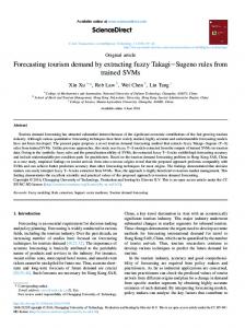
research activities in forecasting with artificial neural networks (ANN) suggest that ANNs can be a promising alternative to the traditional linear methods like (e.g., multiple regression model, ARIMA). In recent years, the study of artificial neural networks (ANN) has aroused great interest in fields just like biology, psychology, medicine, economics, mathematics, statistics and computers (Khashei et al., 2012; Palmer,2006). An Artificial Neural Network (ANN) can be defined as information processing systems whose structure and functioning are inspired by the human brain. In general, an ANN consists of a large number of nodes known also as neurons which in turn are organized in layers. A typical neural network consists of an input layer, representing the independent variables of the problem in separate neurons, and an output layer representing the response variables. The layers in between are referred as hidden layers. They are used in order to increase the model’s flexibility although, Hornik et al. (1989) showed that one hidden layer is sufficient to model any piecewise continuous function. Each neuron can be consider a processing unit connected to other neurons by communication links, known as synapses. To each of the synapses, a weight, , is attached indicating the effect of the corresponding neuron, and all data pass the neural network as signals. The sum of these weighted signals provides the neuron’s total or net input. Then a mathematical function known as activation function, is applied to the net input in order to compute the the neuron’s total output which is sent to other neurons. An example of an ANN with 3 inputs, one hidden layer with 3 neurons and one output is depicted in Figure 1.
Figure 1: An example of ANN Although many types of neural network models have been proposed, the most popular one for time series forecasting is the feed-forward network model (Bishop, 1995). Data enters the network through input layers, moves through hidden layers and exits through output layer. Such an ANN with hidden layers, an input layer with inputs and one an output layer with one output neuron has the following mathematical representation: (1)
MIBES Transactions, Vol 11, Issue 1, 2017
95
Karakitsiou-Mavromati, 92-105
where and are the output and the activation function respectively, denotes the intercept of the output neuron and the intercept of the hidden neuron, represents synaptic weight corresponding to the synapse starting at the hidden neuron and leading to the output neuron, the vector of all synaptic weights corresponding to the synapses leading to the hidden neuron and the vector of all inputs. The activation function is usually a bounded non-decreasing nonlinear and differentiable function such as the logistic function,
(2) The most important feature of an artificial neural network is its ability to learn from their environment and improve their performance through learning. Neural networks are fitted to the data by learning algorithms during a training process. The learning algorithms commonly used in this type of network is back propagation algorithm developed by Rumelhart et al., (1986).
Support Vector Regression (SVR) Support vector machines (SVM) (Boser et. al., 1992; Cortes and Vapnik, 1995; Vapnik et al., 1997) are supervised learning algorithms used for classification and regression analysis. SVMs, build a linear separating hyperplane, by mapping data into the feature space with the higher-dimensional, using the so-called kernel trick. The capacity of the system is controlled by parameters that do not depend on the dimensionality of feature space. One of the most important ideas in Support Vector Classification and Regression cases is that presenting the solution by means of small subset of training points gives enormous computational advantages. Given a training data set where X denotes the space of the input patterns, the prediction for the linear model is given by: (3) where w is the coefficients vector, b is the bias and is the input vector. In the − SVR (Vapnik, 1995) the aim is to find a function, , with at most −deviation from the output y and ensure that it is as flat as possible, i.e one seeks a small . This is formulated as a convex optimization problem to minimize (4) st (5) (6) (7)
MIBES Transactions, Vol 11, Issue 1, 2017
96
Karakitsiou-Mavromati, 92-105
where and are slack variables that allow regression errors to exist up to the value of and , and guarantee at the same time the feasibility of the problem (4)-(7). The constant controls the penalty imposed on observations that lie outside the ε margin and helps to prevent overfitting. This value determines the trade-off between the flatness of and the amount up to which deviations larger than are tolerated. The quality of estimation is measured by the loss function, (8)
It can be shown that the optimization problem (4)-(7) can transformed into the dual problem and its solution is given by (9)
where and are Lagrangian multipliers. The training vectors giving non-zero Lagrange multipliers are called support vectors. Some regression problems cannot adequately be described using a linear model. In such a case, the Lagrange dual formulation allows the technique to be extended to nonlinear functions. The model can be extended to the nonlinear case through the concept of kernel , giving (10) Some popular kernel function used in various application of the SVR are: The Linear Kernel. The Linear kernel is the simplest kernel function. It is given by (11) where is an optional constant. The polynomial kernel. Polynomial kernels are well suited for problems where all the training data is normalized. It is given by: (12) where is the degree of the polynomial kernel, is the slope, and is a constant. The Radial Basis Function (RBF) kernel, or Gaussian kernel (13) The parameter defines how far the influence of a single training example reaches.
MIBES Transactions, Vol 11, Issue 1, 2017
97
Karakitsiou-Mavromati, 92-105
Data and Methodology Data The selection of data for was based on data availability, the reliability of data sources, and the measurability of variables in the modeling process. The data were used for forecasting Greek tourism demand, was set up from the following sources: World Bank Reports; World Travel and Tourism Council; European Central Bank, Statistical Data; Greek National Tourism Organization; Hellenic Statistical Authority; Media Services S.A.; Research Institute of Tourism; Bank of Greece. The variables that will form the basis for construction of the models and will study their behavior for the reporting period (1990 to 2015), are following. The variable number of foreign arrivals in Greece y was used as the dependent variable in the model and will be explained by a set of variables, including: the service price in Greece relative to foreign countries (SP), the population in foreign countries (P), the real gross domestic expenditure per person by country (GDP), the average per capita tourism expenditure in Greece (ACE) the foreign exchange rate (FER) and the marketing expenses to promote Greek tourism industry (MKT). Similar explanatory variables were used in the literature (e.g., Law and Au (1999); Law (2001)). The explanatory variables were selected for five non-EU or non-EURO countries and European countries that do not use euro by using time series between 1996 and 2015 with yearly collected historical data., including: United States of America, Australia, Canada, Sweden and Denmark. In this study, due to data unavailability, ACE was used as a proxy for the cost of living for tourists in Greece, and MKT was used as a proxy for marketing expenses to promote Greek tourism industry. Similarly, GDP was used as a proxy for the income level of foreign tourists, and SP was used as a proxy variable for the relative prices for purchases. All monetary values are measured in US dollars. Following the approach suggested by Law and Au (1999) and Law (2001) for every year and every country , the SP was calculated in the following way:
=
(14)
Data preprocessing Data preprocessing is widely known as an essential step to have the data in a suitable range. It refers to the procedure of analyzing and transforming input and output variables in order to detect the underling components of a time series, underline important relationships and flatten the variable’s distribution. Data preprocessing can have a significant impact on the subsequent forecasting performance. Particularly for the ANN models it prevents node saturation by high input values. During the application of an ANN model it is necessary to normalize the data set in order to allow the range its value to fall inside the work interval of the activation function whose activation values gen-
MIBES Transactions, Vol 11, Issue 1, 2017
98
Karakitsiou-Mavromati, 92-105
erally fall between the [0, 1] or [−1, 1] interval. Depending on the data set, avoiding normalization may lead to overfitting or to a very difficult training process. There different methods to scale the data (z-normalization, min-max normalization, decimal scaling etc). In this work, the data set is normalized in the interval of [0, 1] using the min − max normalization procedure. This measure considerably accelerates weight learning and avoids saturation or overflow of the hidden and output neurons. After the model estimation procedure, the output of the estimated models is converted back to their original scales so that the model fitting and the forecasting performance can be directly compared. Accuracy measures The performance of in-sample fit and out-of-sample forecast is judged by three commonly used error measures. They are the root square percentage error (RMSPE), the mean absolute percentage error (MAPE), and the person and the Person correlation coefficient . The use of these measures represents different angles to evaluate forecasting models. RMSE given by equation (15) is an absolute performance measure closely related to the mean squared error (MSE). MAPE is a relative measurement used for comparison across the testing data because it is easy to interpret, independent of scale, reliable and valid. It is calculate by equation (16). Finally, the correlation given by equation (17) is an indication of the degree of linear association between two numerical variables (15)
(16) (17) where, and represent, respectively, the actual and the estimated value of the depended variable (tourist arrivals in Greece) and is the number of observations used.
Empirical results ANN Model Development The neural network model used in this study is the standard threelayer feedforward network. The input layer consists of 6 neurons (the independent variables described in Section 5.1), we also assume one hidden neuron in the output layer, the number of tourists’ visits in Greece. The hidden layer of an ANN model serves as the connection link between inputs and outputs. Following the findings of Hornik et al. (1989) we assume that one hidden layer is enough in order to construct an approximation function for the tourist demand in Greece. In addition, there is no rule that indicates the optimum number of hidden
MIBES Transactions, Vol 11, Issue 1, 2017
99
Karakitsiou-Mavromati, 92-105
neurons for any given problem. Previous studies (eg., Lenard et al. (1995); Piramuthu et al. (1994)) have shown that the number of neurons in the hidden layer can be up to (1) 2n + 1 (where n is the number of neurons in the input layer), (2) 75% of input neurons, (3) 50% of input and output neurons. In our implementation, adopting the previous suggestions, the range of the hidden neurons is [0, 5, 10, 13] where the model with 0 hidden neurons corresponds essentially to linear model if a linear activation function is employed. The transfer function for hidden neurons is the logistic function and for the output node, the linear function. Bias terms (intersections) are used in both hidden and output layers. To train the multilayer feed-forward neural networks, we employed the backpropagation algorithm developed by Rumelhart et al., (1986). An important parameter of the backpropagation algorithm is the learning rate which controls the amount of changes in weight and reduces the possibility of any weight oscillation during the training cycle. The choice of the learning rate can have a dramatic effect on generalization accuracy as well as the speed of training (Wilson and Martinez,2001). The learning rate we use during the training stage is in the range [0.01, 0.02, 0.03, 0.04, 0.05] for each one the models. The whole procedure of training, validating and testing the resulting models was performed in R (R Core Team, 2016) using the package neuralnet by Fritsch and Guenther (2016). Due to limited amount of data we employed a 10-fold cross-validation approach to select the training and testing data sets. In this process, the data set was randomly divided into 10 folds (subsets); each of the 10 folds contained approximately the same number of data points. In each turn, different 9/10 folds of the data set were used for building a model and the remaining 1-fold alone was used for testing the model. At the end, each instance in the dataset became one time a member of any one of the randomly selected 10 different test folds. Since we randomly generated 10 different test folds in the 10-fold crossvalidation approach, each run generated 10 accuracy estimates. The error estimates of MAPE and RMSE and the values for the 10 different test folds were averaged and reported. SVR Model Development The forecasting accuracy of a SVR model depends on a good setting of parameters C, ε and the kernel parameters. Thus, the determination of this set of parameters is an important issue. However, there is no general systematic method to select parameters used in the SVR model. For training the radial kernel model, which is used in this paper the determination the optimal value of C and parameter γ is required. We explore different values for C [1,10,100,1000], the choice of the optimal for the parameter C is performed during the validation stage. During our training phase γ takes values from the interval [0.01,0.03,0.04,0.05,0.06,0.07,0.1,0.3,0.5,1.3]. The parameter is chosen from the interval [0.01,0.03,0.04, 0.06, 0.07,0.1,0.3,0.8]. The implementation of all the SVR model was performed in R (R Core Team,2016) using the package e1071 by Meyer et all. (2015). The tune.svm() function included in the package e1071 performs a validation process similar to the one we use in the ANN model and returns
MIBES Transactions, Vol 11, Issue 1, 2017
100
Karakitsiou-Mavromati, 92-105
the optimal parameters, where by optimal we mean producing the smallest test error rate. Results In this section, the empirical results for all the countries under study are presented. Figure 2 provides a graphical presentation of these findings.
Figure 2: Graphical representation of the empirical results The accuracy measurements for both methods and all originating countries are presented in Table 1. From these results, it is clear that the machine learning methods do not differ significantly in performance. There is no dominant method which performed the best for all the datasets. Results are quite acceptable considering the small size of the datasets. Most machine learning models require large datasets for model training. Another issue that has to be considered is the economic crisis that happened in mid 2008. It is known that such events perturb the tourism industry with respect to historical trends. This can of course complicate the forecasting problem and affect the performance.
MIBES Transactions, Vol 11, Issue 1, 2017
101
Karakitsiou-Mavromati, 92-105
Table 1:
Accuracy measures for every method by Originating Country
RMSE MAPE
RMSE MAPE
RMSE MAPE
RMSE MAPE
RMSE MAPE
USA ANN Learning rate:0.01 Number of hidden layers: 15 13.9 13.1 0.97 Australia ANN Learning rate:0.02 Number of hidden layers: 15 15.17 14.43 0.98 Canada ANN Learning rate:0.03 Number of hidden layers: 15 15.46 14.98 0.985 Sweden ANN Learning rate:0.03 Number of hidden layers: 10 5.09 5.05 0.97 Denmark ANN Learning rate:0.02 Number of hidden layers: 15 7.72 7.66 0.99
SVR C=100,
13.6 12.9 0.98 SVR C=100,
14.71 13.74 0.98 SVR C=100,
10.75 10.44 0.986 SVR C=100,
9.09 8.99 0.97 SVR C=100,
7.87 7.78 0.99
Conclusion-Future Research This paper has described the process of modeling tourist demand for travel to Greece, using two well established machine learning techniques, namely, Artificial Neural Networks and Support Vector Regression. Data used to build the corresponding models were obtained from several official authorities. These data were randomly separated into a training data set to build the models, and a testing data set to ex-
MIBES Transactions, Vol 11, Issue 1, 2017
102
Karakitsiou-Mavromati, 92-105
amine the level of forecasting accuracy, a 10-fold cross validation procedure was used for this purpose. Exogenous factors that affect the demand of five countries citizens’ for travel to Greece were considered as inputs to the models. The output consisted of the number of visitors from these countries to Greece. Experimental results demonstrated the forecasting efficiency of both models. However, no method that can be considered the best one for all the datasets. To our knowledge this research was a first attempt to model tourists’ demand for travel to Greece using Machine Learning techniques and although this study is limited both in the number of originating countries, time span, and sample sizes, the findings should be of use to tourism practioners and researchers who are interested in forecasting using machine learning methods. Machine learning models were not widely used in tourism demand forecasting except for multi-layer perceptron models. Our findings reflect that machine learning models other than MLP models can give similar performance when the available data are very small. A possibility for future research could be to include some qualitative exogenous variables, for example government policies, international conditions, natural disasters etc. play an important role in determining tourist arrivals, leading to a notable change in demand for tourism. However, these qualitative factors are dynamic in a continuous way. A major challenge for including qualitative factors would be to provide a commonly acceptable measurement for these factors.
References Adhikari, R. & Agrawal, R.K., (2012), Forecasting strong seasonal time series with artificial neural networks, Journal of Scientific & Industrial Research, 71, 657-666. Andrew, W.P., Crange, D.A. & Lee, C.K., (1990), Forecasting hotel occupancy rates with time series models: A empirical analysis, Hospitality Research Journal, 14(2), 173–181. Bishop, C.M., (1995), Neural networks for pattern recognition, Oxford University Press, Oxford. Boser B.E., Guyon I.M. & Vapnik V.N., (1992), A training algorithm for optimal margin classifiers, In: Haussler D. (Ed.), Proceedings of the Annual Conference on Computational Learning Theory, ACM Press, Pittsburgh, PA, 144-152. Box, G.E.P. & Jenkins, G.M., (1970), Time Series Analysis, Forecasting and Control San Francisco: Holden Day. Chan F., Lim C. & McAleer M., (2005), Modelling multivariate international tourism demand and volatility, Tourism Management, 26, 459471. Chen, C.F., Lai, M.C. & Yeh, C.C., (2012), “Forecasting tourism demand based on empirical mode decomposition and neural network,” Knowledge-Based Systems, 26, 281-287. Cho V., (2001), Tourism forecasting and its relationship with leading economic indicators, Journal of Hospitality and Tourism Research, 25, 399-420. Claveria, O. & Torra, S., (2014), Forecasting tourism demand to Catalonia: Neural networks vs. time series models, Economic Modelling, 36, 220-228. Coshall J., (2006), Time series analyses of UK outbound travel by Air, Journal of Travel Research, 44, 335-347. Cortes C. & Vapnik V., (1995), Support vector networks Machine Learning, 20, 273–297.
MIBES Transactions, Vol 11, Issue 1, 2017
103
Karakitsiou-Mavromati, 92-105
Clements, M.P. & Hendry, D.F., (1998), Forecasting economic time series, Cambridge, Cambridge University Press. Fernando, H., Turner, L.W. & Reznik, L., (1999), Neural networks to forecast tourist arrivals to Japan from the USA, Paper presented at Third International Data Analysis Symposium, Aachen, 17 September. Fritsch, S. & Guenther, F., (2016), neuralnet: Training of Neural Networks R package version 1.33, https://CRAN.Rproject.org/package=neuralnet Goh, C. & Law, R., (2002), “Modeling and forecasting tourism demand for arrivals with stochastic nonstationary seasonality and intervention,” Tourism Management, 23(5), 499-510. Hornik, K., Stichcombe, M. & White, H., (1989), “Multi-layer feedforward networks are universal approximators,” Neural Networks, 2, 359–366. Khashei, M., Hamadani. A. & Bijari, M., (2012), “A novel hybrid classification model of artificial neural networks and multiple linear regression models,” Expert Systems with Applications, 39(3), 26062620. Khashei, M., Hejazi, S. & Bijari, M., (2008), “A new hybrid artificial neural networks and fuzzy regression model for time series forecasting,” Fuzzy Sets and Systems, 159(7), 769-786. Kulendran, N. & Wilson, K., (2000), Modelling business travel, Tourism Economics, 6, 47-59. Law, R., (2001), “The impact of the Asian financial crisis on Japanese demand for travel to Hong Kong: a study of various forecasting techniques,” Journal of Travel and Tourism Marketing, 10, 47-66. Law, R. & Au, N., (1999), “A neural network model to forecast Japanese demand for travel to Hong Kong,” Tourism Management, 20(1), 89-97. Lenard, M.J, Alam, P. & Madey, G.R., (1995), “The application of neural networks and a qualitative response model to the auditors going concern uncertainty decision,” Decision Science, 26, 209–227. Li, G., Wong, K.F., Song, H. & Witt, S.F., (2006), “Tourism demand forecasting: A time varying parameter error correction model,” Journal of Travel Research, 45, 175-185. Lim, C. & McAleer, M., (2001), “Cointegration analysis of quarterly tourism demand by HongKong and Singapore for Australia,” Applied Economics, 33, 1599-1619. Martin, C.A. & Witt, S.F., (1989), “Accuracy of econometric forecasts of touris,” Annals of tourism Research, 16(3), 407–428. Meyer, D., Dimitriadou, E., Hornik, K., Weingessel, A. & Leisch, F., (2015), e1071: Misc Functions of the Department of Statistics, Probability Theory Group (Formerly: E1071), TU Wien. R package version 1.6-7, https://CRAN.Rproject.org/package=e1071 Palmer, A., Montano, J.J. & Ses, A., (2006), “Designing an artificial neural network for forecasting tourism time series,” Tourism Management, 27(5), 781-790. Pattie, D.C. & Snyder, J., (1996), “Using a neural network to forecast visitor behavior,” Annals of Tourism Research, 23, 151-164. Piramuthu, S., Shaw, M. & Gentry, J., (1994), “A classification approach using multilayered neural networks,” Decision Support Systems, 11, 509–525 R Core Team, (2016), R: A language and environment for statistical computing, R Foundation for Statistical Computing, Vienna, Austria. URL https://www.Rproject.org/. Rumelhart, D.E., Hinton, G.E. & Williams, R.J., (1986), Learning internal representations by error propagation. In D. E. Rumelhart, and J. L. McClelland (Eds.), Parallel distributed processing, MIT Press, Cambridge, MA, 318-362.
MIBES Transactions, Vol 11, Issue 1, 2017
104
Karakitsiou-Mavromati, 92-105
Shan, J. & Wilson, K., (2001), “Causality between trade and tourism : Empirical evidence from China,” Applied Economics Letters, 8, 279283. Song, H. & Li, G., (2008), “Tourism demand modelling and forecastinga review of recent research,” Tourism Management, 29, 203-220. Song, H. & Turner, L., (2006), Tourism demand forecasting, in Dwyer, L., and Forsyt, P. (eds) International Handbook on the Economics of Tourism, Edward Elgar, Cheltenham. Song, H. & Witt, S.F., (2000), Tourism Demand Modeling and Forecasting: modern econometric approaches, Pergamon, Cambridge. Song, H. & Witt, S.F., (2006), “Forecasting international tourist flows to Macau,” Tourism Management, 27, 214-224. Song, H., Witt, S. F. & Jensen, T.C., (2003), “Tourism forecasting: Accuracy of alternative econometric models,” International Journal of Forecasting, 19, 123-141. Teixeira, J. & Fernandes P., (2014), “Tourism time series forecast with artificial neural networks,” Review of Applied Management Studies, 12, 26-36. Tsaur, S.H., Chiu, Y.C. & Huang, C.H., (2002), “Determinants of guest loyalty to international tourist hotels: a neural network approach,” Tourism Management, 23, 397-405. Uysal, M. & El Roubi, M.S., (1999), “Artificial neural Networks versus multiple regression in tourism demand analysis,” Journal of Travel Research, 38, 111-118. Vapnik, V., (1995), The nature of stastical learning theory, Springer, NY. Vapnik, V., Golowich, S. & Smola, A., (1997), Support vector method for function approximation, regression estimation, and signal processing In: Mozer M.C., Jordan M.I., and Petsche T. (Eds.) Advances in Neural Information Processing Systems 9, MA, MIT Press, Cambridge, 281–287. Wilson, D.R. & Martinez R.T., (2001), The Need for Small Learning Rates on Large Problems in Proceedings of the 2001 International Joint Conference on Neural Networks (IJCNN01), 115– 119 Witt, S.F. & Witt, C.A., (1995), “Forecasting tourism demand: a review of empirical research,” International Journal of Forecasting, 11, 447-475. WTTC, (2015), Greece: Travel and Tourism Economic Impact, London: World Travel and Tourism Council. Zhang, G.P., (2003), “Time series forecasting using a hybrid ARIMA and neural network model,” Neurocomputing, 50, 159-175.
MIBES Transactions, Vol 11, Issue 1, 2017
105