Nathalie Japkowicz School of Electrical Engineering & Computer Science University of Ottawa
[email protected]
Motivation: My story A student and I designed a new algorithm for data that
had been provided to us by the National Institute of Health (NIH). According to the standard evaluation practices in machine learning, we found our results to be significantly better than the state-of-the-art. The machine learning community agreed as we won a best paper award at ISMIS’2008 for this work. NIH disagreed and would not consider our algorithm because it was probably not truly better than the others. 2
Motivation: My story (cont’d) My reactions were: Surprise: Since my student and I properly applied the evaluation methodology that we had been taught and read about everywhere, how could our results be challenged? Embarrassment: There is obviously much more to evaluation than what I have been told. How can I call myself a scientist and not know what the scientists of other fields know so well? Determination: I needed to find out more about this and share it with my colleagues and students. 3
Information about this tutorial This tutorial is based on the book I have co-written
after going through the experience I just described. It will give you an overview of the complexity and uncertainty of evaluation. It will also give you a brief overview of the issues that come up in different aspects of evaluation and what the possible remedies may be. Finally, it will direct you to some resources available that can help you perform more robust evaluations of your systems. 4
Book Details Evaluating Learning Algorithms: A Classification Perspective Nathalie Japkowicz & Mohak Shah Cambridge University Press, 2011
Review:
"This treasure-trove of a book covers the important topic of performance evaluation of machine learning algorithms in a very comprehensive and lucid fashion. As Japkowicz and Shah point out, performance evaluation is too often a formulaic affair in machine learning, with scant appreciation of the appropriateness of the evaluation methods used or the interpretation of the results obtained. This book makes significant steps in rectifying this situation by providing a reasoned catalogue of evaluation measures and methods, written specifically for a machine learning audience and accompanied by concrete machine learning examples and implementations in R. This is truly a book to be savoured by machine learning professionals, and required reading for Ph.D students." Peter A. Flach, University of Bristol
5
The main steps of evaluation
6
What these steps depend on These steps depend on the purpose of the evaluation: Comparison of a new algorithm to other (may be generic or application-specific) classifiers on a specific domain (e.g., when proposing a novel learning algorithm) Comparison of a new generic algorithm to other generic ones on a set of benchmark domains (e.g. to demonstrate general effectiveness of the new approach against other approaches) Characterization of generic classifiers on benchmarks domains (e.g. to study the algorithms' behavior on general domains for subsequent use) Comparison of multiple classifiers on a specific domain (e.g. to find the best algorithm for a given application task)
Outline of the tutorial: Part I (from now until the coffee break!) Choosing a performance measure. Choosing a statistical test. Part II (from after the coffee break to the lunch break!) What about sampling? What data sets should we use? Available resources Part III (if there is time before lunch and we’re not too
hungry!)
Recent research 8
Topic 1: Choosing a Performance Measure
9
Which Classifier is better? Almost as many answers as there are performance measures! (e.g., UCI Breast Cancer) Algo
Acc
RMSE TPR
FPR
Prec
Rec
F
AUC
Info S
NB
71.7
.4534
.44
.16
.53
.44
.48
.7
48.11
C4.5
75.5
.4324
.27
.04
.74
.27
.4
.59
34.28
3NN
72.4
.5101
.32
.1
.56
.32
.41
.63
43.37
Ripp
71
.4494
.37
.14
.52
.37
.43
.6
22.34
SVM
69.6
.5515
.33
.15
.48
.33
.39
.59
54.89
Bagg
67.8
.4518
.17
.1
.4
.17
.23
.63
11.30
Boost
70.3
.4329
.42
.18
.5
.42
.46
.7
34.48
RanF
69.23
.47
.33
.15
.48
.33
.39
.63
20.78
10
Which Classifier is better? Ranking the results Algo
Acc
RMSE TPR
FPR
Prec
Rec
F
AUC
Info S
NB
3
5
1
7
3
1
1
1
2
C4.5
1
1
7
1
1
7
5
7
5
3NN
2
7
6
2
2
6
4
3
3
Ripp
4
3
3
4
4
3
3
6
6
SVM
6
8
4
5
5
4
6
7
1
Bagg
8
4
8
2
8
8
8
3
8
Boost
5
2
2
8
7
2
2
1
4
RanF
7
6
4
5
5
4
7
3
7
11
What should we make of that? Well, for certain pairs of measures, that makes sense,
since each measure focuses on a different aspect of learning.
For example, the TPR and the FPR are quite different, and
often, good results on one yields bad results on the other. Precision and Recall also seem to tradeoff each other.
How about the global measures (Acc, RMSE, the F-
measure, AUC, the Information Score)?
They too disagree as they each measure different (though
more difficult to pinpoint as they are composite measures) aspects of learning.
12
Is this a problem? It is not a problem when working on a specific
application since the purposes of the application are clear and the developer knows which performance measure is best to optimize in that context. It does become a problem, however, when the general usefulness of a new algorithm is assessed. In that case, what performance measure should be chosen? If only one or a few measures are chosen, then it can be
argued that the analysis is incomplete, and misleading. If many measures are chosen, the results become too mitigated for any clear statement to be issued.
13
What to do, then? One suggestion which tries to balance pragmatics
(getting the paper accepted!) with fairness (acknowledging the weakness of the new algorithm!) is to divide the evaluation procedure into two parts: In the first part, choose a few important metrics on which
the new method excels in order to demonstrate this new method’s worth. In a second part, overview the results that the new method obtains on a large selection of performance measures. Try to explain these observations; do not be too strict (i.e., if the new method
consistently ranks as one of the best three methods tested, then it is not that bad. Similarly, if it ranks very badly on only one performance measure, then it is not that bad either). 14
Overview of Performance Measures
15
A Few Confusion Matrix-Based Performance Measures Accuracy = True class Hypothesized | class V
Pos
Neg
Yes
TP
FP
No
FN
TN
P=TP+FN
N=FP+TN
A Confusion Matrix
(TP+TN)/(P+N) Precision = TP/(TP+FP) Recall/TP rate = TP/P FP Rate = FP/N ROC Analysis moves the threshold between the positive and negative class from a small FP rate to a large one. It plots the value of the Recall against that of the FP Rate at each FP Rate considered. 16
Issues with Accuracy True class
Pos
Neg
True class
Pos
Neg
Yes
200
100
Yes
400
300
No
300
400
No
100
200
P=500
N=500
P=500
N=500
Both classifiers obtain 60% accuracy They exhibit very different behaviours: On the left: weak positive recognition rate/strong negative recognition rate On the right: strong positive recognition rate/weak negative recognition rate 17
Issues with Precision/Recall True class
Pos
Neg
True class
Pos
Neg
Yes
200
100
Yes
200
100
No
300
400
No
300
0
P=500
N=500
P=500
N=100
Both classifiers obtain the same precision and recall values of 66.7% and 40% (Note: the data sets are different) They exhibit very different behaviours: Same positive recognition rate Extremely different negative recognition rate: strong on the left / nil on the right Note: Accuracy has no problem catching this! 18
Is the AUC the answer? Many researchers have now adopted the AUC (the area
under the ROC Curve). The principal advantage of the AUC is that it is more robust than Accuracy in class imbalanced situations. Indeed, given a 95% imbalance (in favour of the negative class, say), the accuracy of the default classifier that issues “negative” all the time will be 95%, whereas a more interesting classifier that actually deals with the issue, is likely to obtain a worse score. The AUC takes the class distribution into consideration. 19
Is the AUC the Answer? (cont’) While the AUC has been generally adopted as a
replacement for accuracy, it met with a couple of criticisms: The ROC curves on which the AUCs of different classifiers
are based may cross, thus not giving an accurate picture of what is really happening. The misclassification cost distributions (and hence the skew-ratio distributions) used by the AUC are different for different classifiers. Therefore, we may be comparing apples and oranges as the AUC may give more weight to misclassifying a point by classifier A than it does by classifier B (Hand, 2009) Answer: the H-Measure, but it has been criticized too!
20
Some other measures that will be discussed in this tutorial: Deterministic Classifiers: Chance Correction: Cohen’s Kappa
Scoring Classifiers: Graphical Measures: Cost Curves (Drummond & Holte,
2006) Probabilistic Classifiers: Distance measure: RMSE Information-theoretic measure: Kononenko and Bratko’s Information Score Multi-criteria Measures: The Efficiency Method (Nakhaeizadeh & Schnabl, 1998)
21
Cohen’s Kappa Measure Agreement Statistics argue that accuracy does not take
into account the fact that correct classification could be a result of coincidental concordance between the classifier’s output and the label-generation process. Cohen’s Kappa statistics corrects for this problem. Its formula is: κ = (P0 – PeC )/ ( 1 – PeC)
where
P0 represents the probability of overall agreement over the label
assignments between the classifier and the true process, and PeC represents the chance agreement over the labels and is defined as the sum of the proportion of examples assigned to a class times the proportion of true labels of that class in the data set. 22
Cohen’s Kappa Measure: Example Predicted -> Actual
A
B
C
Total
A
60
50
10
120
B
10
100
40
150
C
30
10
90
130
Total
100
160
140
Accuracy = P0 = (60 + 100 + 90) / 400 = 62.5% PeC = 100/400 * 120/400 + 160/400 * 150/400 + 140/400 * 130/400 = 0.33875 κ = 43.29% Accuracy is overly optimistic in this example! 23
Cost Curves
Cost-curves are more practical than ROC curves because they tell us for what class probabilities one classifier is preferable over the other.
ROC Curves only tell us that sometimes one classifier is preferable over the other 24
RMSE The Root-Mean Squared Error (RMSE) is usually used
for regression, but can also be used with probabilistic classifiers. The formula for the RMSE is: RMSE(f) = sqrt( 1/m Σi=1m(f(xi) – yi)2)) where m is the number of test examples, f(xi), the classifier’s probabilistic output on xi and yi the actual label.
ID
RMSE(f f(xi) )yRMSE(f (f(xi))– yi)2 i
1
.95
1
.0025
2
.6
0
.36
3
.8
1
.04
4
.75
0
.5625
5
.9
1
.01
RMSE(f) = sqrt(1/5 * (.0025+.36+.04+.5625+.01)) = sqrt(0.975/5) = 0.4416
25
Information Score Kononenko and Bratko’s Information Score assumes a prior P(y) on the
labels. This could be estimated by the class distribution of the training data. The output (posterior probability) of a probabilistic classifier is P(y|f), where f is the classifier. I(a) is the indicator fonction. IS(x) = I(P(y|f) ≥ P(y)) * (-log(P(y))+log(P(y|f)) + + I(P(y|f) < P(y)) * (- log(1-P(y))+log(1-P(y|f))) ISavg= 1/m Σi=1m(IS(xi)) x
P(yi|f ) yi
IS(x)
1
.95
1
0.66
2
.6
0
0
3
.8
1
.42
4
.75
0
.32
5
.9
1
.59
P(y=1) = 3/5 = 0.6 P(y=0) = 2/5 = 0.4 IS(x1) = 1 * (-log(.6) + log(.95)) + 0 * (-log(.4) + log).05)) = 0.66
ISavg= 1/5 (0.66+0+.42+.32+.59) = 0.40 26
Efficiency Method The efficiency method is a framework for combining
various measures including qualitative metrics, such as interestingness. It considers the positive metrics for which higher values are desirable (e.g, accuracy) and the negative metrics for which lower values are desirable (e.g., computational time).
εS(f)= Σiwipmi+(f) / Σ w nm (f) j
j
j
pmi+ are the positive metrics and nmj- are the negative metrics. The wi’s and wj’s have to be determined and a solution is proposed that uses linear programming. 27
Topic 2: Choosing a Statistical Test
28
The purpose of Statistical Significance Testing The performance metrics just discussed allow us to
make observations about different classifiers. The question we ask here is: can the observed results be attributed to real characteristics of the classifiers under scrutiny or are they observed by chance? The purpose of statistical significance testing is to help us gather evidence of the extent to which the results returned by an evaluation metric are representative of the general behaviour of our classifiers.
29
Hypothesis Testing Hypothesis testing consists of stating a null hypothesis which usually is
the opposite of what we wish to test (for example, classifiers A and B perform equivalently) We then choose a suitable statistical test and statistic that will be used to reject the null hypothesis. We also choose a critical region for the statistic to lie in that is extreme enough for the null hypothesis to be rejected. We calculate the observed test statistic from the data and check whether it lies in the critical region. If so, reject the null hypothesis. If not, we fail to reject the null hypothesis, but do not accept it either. Rejecting the null hypothesis gives us some confidence in the belief that our observations did not occur merely by chance.
30
Issues with Hypothesis Testing Hypothesis testing never constitutes a proof that our observation is valid.
It provides added support for our observations. We can never be 100% sure about them. Statistical tests come in two forms: parametric and non parametric. Parametric tests make strong assumptions about the distribution of the underlying data. Non-parametric ones make weaker assumptions about the data, but are also typically less powerful (less apt at rejecting the null hypothesis when it is false) than their parametric counterparts. It is often difficult, if not impossible, to verify that all the assumptions hold. The results of statistical tests are often misinterpreted: (1-p) does not represent P(H|D)
(1-p) does not represent the probability of replication of successful replication
of the observations
It is always possible to show that a difference between two alternatives,
no matter how small, is significant, provided that enough data is used.
31
To test or not to test? Given the serious issues associated with statistical testing, some
researchers (Drummond, 2006, Demsar, 2008) argue that Machine Learning and Data Mining researchers should drop the habit of performing statistical tests. They argue that, this process: Overvalues the results, and Limits the search for novel ideas (because of the excess (not always warranted) confidence in the results). The alternative, however, is to train researchers properly in the understanding and application of statistical methods, so that they can decide on their own when a statistical test is warranted, what its limitations are and when the search for new ideas is necessary. 32
How to choose a statistical test? There are several aspects to consider when choosing a
statistical test.
What kind of problem is being handled? Whether we have enough information about the
underlying distributions of the classifiers’ results to apply a parametric test?
Regarding the type of problem, we distinguish between The comparison of 2 algorithms on a single domain The comparison of 2 algorithms on several domains The comparison of multiple algorithms on multiple domains 33
Statistical tests overview
34
Statistical Tests we will describe and illustrate in this tutorial Two classifiers, one domain: The t-test (parametric) McNemar’s test (non-parametric) The Sign Test
Two classifiers, multiple domains The Sign Test (non-parametric) Wilcoxon’s signed-Rank Test (non-parametric)
Multiple classifiers, multiple domains: Friedman’s Test (non-parametric) The Nemenyi Test
We will also discuss and illustrate the concept of the effect size. 35
Two classifiers, one domain The t-test (parametric) McNemar’s test (non-parametric) The Sign Test (usually used for multiple domains but
can also be used on a single domain).
36
The (2-matched samples) t-test Given two matched samples (e.g., the results of two
classifiers applied to the same data set with matching randomizations and partitions), we want to test whether the difference in means between these two sets is significant. In other words, we want to test whether the two samples come from the same population. We look at the difference in observed means and standard deviation. We assume that the difference between these means is zero (the null hypothesis) and see if we can reject this hypothesis. 37
The t-statistic
The degree of freedom is n-1 = 9; Using a 2-sided test, the null hypothesis can therefore be rejected at the 0.001 significance level (since the obtained t has to be greater than 4.781for that to be possible). 38
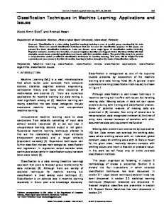
Assumptions of the t-test The Normality or Pseudo-Normality Assumption: The t-test requires that
the samples come from normally distributed population. Alternatively, the sample size of the testing set should be greater than 30. The Randomness of the Samples: The sample should be representative of the underlying population. Therefore, the instances of the testing set should be randomly chosen from their underlying distribution. Equal Variance of the populations: The two sample come from populations with equal variance. Labour Example: Normality: The labour data set contains only 57 instances altogether. At each
fold of the CV process, only 6 or 7 data points are tested. However, since each trial is a run of 10-fold CV, all 57 examples are tested, so we may be able to assume pseudo-normality. Randomness: The labour data was collected in the 1987-1988 period. All the collective agreements for this period were collected. There is no reason to assume that 1987-1988 was a non-representative year, so we assume that the data was randomly collected. 39
Assumptions of the t-test (cont’d) Equal Variance: The variance of C4.5 (1) and NB (1) cannot be considered equal. (See figure)
We were not warranted to use the t-test to compare C4.5 to NB on the Labour data. A better test to use in this case is the nonparametric alternative to the t-test: McNemar’s Test (See Japkowicz & Shah, 2011 for a description) 40
McNemar’s test
41
The Sign Test Since the Sign test is usually used on multiple domains
(though can be used on a single one with several trial (e.g., 10 folds of cross-validation)), we will discuss it in the next section which looks at multiple domains.
42
Two classifiers multiple domains There are no clear parametric way to deal with the problem
of comparing the performance of two classifiers on multiple domains:
The t-test is not a very good alternative because it is not clear that we have commensurability of the performance measures in such a setting. The normality assumption is difficult to establish as the number of domains on which the test is run must exceed 30. The t-test is susceptible to outliers, which is more likely when many different domains are considered.
Therefore we will describe two non-parametric alternatives
The Sign Test Wilcoxon’s signed-Rank Test 43
The Sign test The sign test can be used either to compare two classifiers
on a single domain (using the results at each fold as a trial) or more commonly, to compare two classifiers on multiple domains. We count the number of times that f1 outperforms f2, nf1 and the number of times that f2 outperforms f1, nf2. The null hypothesis (stating that the two classifiers perform equally well) holds if the number of wins follows a binomial distribution. Practically speaking, a classifier should perform better on at least wα datasets to be considered statistically significantly better at the α significance level, where wα is the critical value for the sign test at the α significance level . 44
Illustration of the sign test
• •
Dataset
NB
SVM
Adaboost
Rand Forest
Anneal
96.43
99.44
83.63
99.55
Audiology
73.42
81.34
46.46
79.15
Balance Scale
72.30
91.51
72.31
80.97
Breast Cancer
71.70
66.16
70.28
69.99
Contact Lenses
71.67
71.67
71.67
71.67
Pima Diabetes
74.36
77.08
74.35
74.88
Glass
70.63
62.21
44.91
79.87
Hepatitis
83.21
80.63
82.54
84.58
Hypothyroid
98.22
93.58
93.21
99.39
Tic-Tac-Toe
69.62
99.90
72.54
93.94
NB vs SVM: nf1= 4.5, nf2= 5.5 and w0.05 = 8 we cannot reject the null hypothesis stating that NB and SVM perform similarly on these data sets for level α=0.05 (1-tailed) Ada vs RF: nf1=1 and nf2=8.5 we can reject the null hypothesis at level α=0.05 (1-tailed) and conclude that RF is significantly better than Ada on these data sets at that significance45level.
Wilcoxon’s signed-Rank Test Wilcoxon’s signed-Rank Test, like the sign test, deals with two
classifiers on multiple domains. It is also non-parametric, however, it is more powerful than the sign test. Here is its description:
For each domain, we calculate the difference in performance of the two
classifiers. We rank the absolute values of these differences and graft the signs in front of the ranks. We calculate the sum of positive and negative ranks, respectively (WS1 and WS2) TWilcox = min(WS1 ,WS2) Compare to critical value Vα. If Vα ≥ TWilcox we reject the null hypothesis that the performance of the two classifiers is the same, at the α confidence level. 46
Wilcoxon’s signed-Rank Test: Illustration Data
NB
SVM
NB-SVM
|NB-SVM| Ranks
1
.9643
.9944
-0.0301
0.0301
3
-3
2
.7342
.8134
-0.0792
0.0792
6
-6
3
.7230
.9151
-0.1921
0.1921
8
-8
4
.7170
.6616
+0.0554
0.0554
5
+5
5
.7167
.7167
0
0
Remove
Remove
6
.7436
.7708
-0.0272
0.0272
2
-2
7
.7063
.6221
+0.0842
0.0842
7
+7
8
.8321
.8063
+0.0258
0.0258
1
+1
9
.9822
.9358
+0.0464
0.0464
4
+4
10
.6962
.9990
-0.3028
0.3028
9
-9
WS1 = 17 and WS2 = 28 TWilcox = min(17, 28) = 17 For n= 10-1 degrees of freedom and α = 0.005, V = 8 for the 1-sided test. V must be larger than TWilcox in order to reject the hypothesis. Since 17 > 8, we cannot reject the hypothesis that NB’s 47 performance is equal to that of SVM at the 0.005 level.
Multiple classifiers, Multiple Domains For the case of multiple classifiers and multiple domains, two
alternatives are possible. The parametric alternative is (one-way repeated measure) ANOVA and the non-parametric alternative is Friedman’s Test. These two tests are multiple-hypothesis tests, also called Omnibus tests. Their null hypotheses is that all the classifiers perform equally, and rejection of that null hypothesis means that: there exists at least one pair of classifiers with significantly different performances. In case of rejection of this null hypothesis, the omnibus test is followed by a Post-hoc test whose job is to identify the significantly different pairs of classifiers. In this tutorial, we will discuss Friedman’s Test (omnibus) and the Nemenyi test (post-hoc test).
48
Friedman’s Test
49
Illustration of the Friedman test Domain
Classifier fA
Classifier fB
Classifier fC
Domain
Classifier fA
Classifier fB
Classifier fC
1
85.83
75.86
84.19
1
1
3
2
2
85.91
73.18
85.90
2
1.5
3
1.5
3
86.12
69.08
83.83
3
1
3
2
4
85.82
74.05
85.11
4
1
3
2
5
86.28
74.71
86.38
5
2
3
1
6
86.42
65.90
81.20
6
1
3
2
7
85.91
76.25
86.38
7
2
3
1
8
86.10
75.10
86.75
8
2
3
1
9
85.95
70.50
88.03
9
2
3
1
19
86.12
73.95
87.18
10
2
3
1
R .j
15.5
30
14.5
50
The Nemenyi test
51
Illustration of the Nemenyi Test
52
Effect Size
53
Topic 1: Sampling
54
What is the Purpose of Resampling? Ideally, we would have access to the entire population
or a lot of representative data from it. This is usually not the case, and the limited data available has to be re-used in clever ways in order to be able to estimate the error of our classifiers as reliably as possible, i.e., to be re-used in clever ways in order to obtain sufficiently large numbers of samples. Resampling is divided into two categories: Simple resampling (where each data point is used for testing only once) and Multiple re-sampling (which allows the use of the same data point more than once for testing) 55
What are the dangers of Resampling? Re-sampling is usually followed by Statistical testing.
Yet statistical testing relies on the fundamental assumption that the data used to obtain a sample statistics must be independent. However, if data is re-used, then this important independence assumption is broken and the result of the statistical test risks being invalid. In addition to discussing a few re-sampling approaches, we will underline the issues that may arise when applying them. 56
Overview of Re-Sampling Methods
57
Resampling Approaches Discussed in this Tutorial Simple Resampling: Cross-Validation and its variants Multiple Resampling: The 0.632 Bootstrap The Permutation Test Repeated k-fold Cross-Validation
58
k-fold Cross-Validation Fold 1:
Fold 2:
….. Fold k-1: Fold k:
: training data subset : testing data subset In Cross-Validation, the data set is divided into k folds and at each iteration, a different fold is reserved for testing and all the others, used for training the classifiers. 59
Some variations of Cross-Validation Stratified k-fold Cross-Validation: This variation is useful when the class-distribution of the data is skewed. It ensures that the distribution is respected in the training and testing sets created at every fold. This would not necessarily be the case if a pure random process were use. Leave-One-Out In k-fold Cross-Validation, each fold contains m/k data points where m is the overall size of the data set. In Leave-one-out, k =m and therefore, each fold contains a single data point. 60
Considerations about k-fold CrossValidation and its variants k-fold Cross-Validation is the best known and most
commonly used resampling technique. K-fold Cross-Validation is less computer intensive than Leave-One-Out. The testing sets are independent of one another, as required, by many statistical testing methods, but the training sets are highly overlapping. This can affect the bias of the error estimates. Leave-One-Out produces error estimates with high variance given that the testing set at each fold contains only one example. The classifier is practically unbiased since each fold trains on almost all the data.
61
Boootsrapping Bootstrapping assumes that the available sample is
representative and creates a large number of new samples by drawing from replacement from the available sample. Bootstrapping is useful in practice when the sample is too small for Cross-Validation or Leave-One-Out approaches to yield a good estimate There are two Bootstrap estimates that are useful in the context of classification: the Є0 and the e632 Bootstrap. The Є0 Bootstrap tends to be pessimistic because it is only trained on 63.2% of the data in each run. The e632 attempts to correct for this. 62
The Є0 and e632 Bootstraps
63
Considerations about Bootstrapping
64
The Permutation Test Given the error estimate found on a data set, the question is: Is this error estimate significant, or Could it also have been obtained on ‘bogus’ data?
The ‘bogus’ data is created by taking the genuine samples and
randomly choosing to either leave their label intact or switch them. Once this ‘bogus’ data set is created, the classifier is ran on it and its error estimated. This process is repeated a very large number of times in an attempt to establish whether the error estimate obtained on the true data is truly different from those obtained on large numbers of ‘bogus’ data sets.
Repeated k-Fold Cross-Validation(1) In order to obtain more stable estimates of an
algorithm’s performance, it is useful to perform multiple runs of simple re-sampling schemes. This can also enhance replicability of the results. Two specific schemes have been suggested in the context of Cross-Validation: 5x2 CV and 10x10 CV K-fold CV does not estimate the mean of the difference between 2 learning algorithms properly. The mean at a single fold behaves better. This lead Dietterich (1998) to propose the 5x2 CV fold, in which 2-fold CV is repeated 5 times. 66
Repeated k-Fold Cross-Validation(2) Dietterich found that the paired t-test based on the the
5x2 CV scheme had lower probability of issuing a type-I error but had less power than the k-fold CV paired t-test. Alpaydyn (1999) proposed to substitute the t-test at the end of the 5x2CV scheme by an F-test. That test had an even lower chance of issuing a type-I error and had increased power (though that new test was not compared to k-fold CV in terms of type I error or power) Bouckaert (2003) proposed several variations of a 10x10 CV scheme. Generally speaking these schemes show a higher probability of Type-I error than 10-fold CV, but higher power. 67
Topic 2: Choosing Appropriate Data Sets for Testing Classifiers
68
Considerations to keep in mind while choosing an appropriate test bed Wolpert’s “No Free Lunch” Theorems: if one algorithm
tends to perform better than another on a given class of problems, then the reverse will be true on a different class of problems. LaLoudouana and Tarate (2003) showed that even mediocre learning approaches can be shown to be competitive by selecting the test domains carefully. The purpose of data set selection should not be to demonstrate an algorithm’s superiority to another in all cases, but rather to identify the areas of strengths of various algorithms with respect to domain characteristics or on specific domains of interest. 69
Where can we get our data from? Repository Data: Data Repositories such as the UCI
repository and the UCI KDD Archive have been extremely popular in Machine Learning Research. Artificial Data: The creation of artificial data sets representing the particular characteristic an algorithm was designed to deal with is also a common practice in Machine Learning Web-Based Exchanges: Could we imagine a multidisciplinary effort conducted on the Web where researchers in need of data analysis would “lend” their data to macine learning researchers in exchange for an analysis? 70
Pros and Cons of Repository Data Pros: Very easy to use: the data is available, already processed and the
user does not need any knowledge of the underlying field. The data is not artificial since it was provided by labs and so on. So in some sense, the research is conducted in real-world setting (albeit a limited one) Replication and comparisons are facilitated, since many researchers use the same data set to validate their ideas. Cons: The use of data repositories does not guarantee that the results will generalize to other domains. The data sets in the repository are not representative of the data mining process which involves many steps other than classification. Community experiment/Multiplicity effect: since so many experiments are run on the same data set, by chance, some will yield interesting (though meaningless) results
71
Pros and Cons of Artificial Data Pros: Data sets can be created to mimic the traits that are expected to be
present in real data (which are unfortunately unavailable) The researcher has the freedom to explore various related situations that may not have been readily testable from accessible data. Since new data can be generated at will, the multiplicity effect will not be a problem in this setting. Cons: Real data is unpredictable and does not systematically behave according to a well defined generation model. Classifiers that happen to model the same distribution as the one used in the data generation process have an unfair advantage. 72
Pros and Cons of Web-Based Exchanges Pros: Would be useful for three communities:
Domain experts, who would get interesting analyses of their problem Machine Learning researchers who would be getting their hand on interesting data, and thus encounter new problems Statisticians, who could be studying their techniques in an applied context.
Cons: It has not been organized. Is it truly feasible? How would the quality of the studies be controlled? 73
Topic 3: Available Resources
74
What help is available for conducting proper evaluation? There is no need for researchers to program all the code necessary to
conduct proper evaluation nor to do the computations by hand. Resources are readily available for every steps of the process, including: Evaluation metrics Statistical tests Re-sampling And of course, Data repositories Pointers to these resources and explanations on how to use them are discussed in our book: . 75
Where to look for evaluation metrics? Actually, as most people know, Weka is a great source for, not only, classifiers, but also computation of the results according to a variety of evaluation metrics
76
WEKA even performs ROC Analysis and draws Cost-Curves
Although better graphical analysis packages are available in R, namely the ROCR package, which permits the visualization of many versions of ROC and Cost Curves, and also Lift curves, P-R Curves, and so on 77
Where to look for Statistical Tests? The R Software Package contains implementations of all the statistical tests discussed here and many more. They are very simple to run.
78
Where to look for Re-sampling methods? In our book, we have implemented all the re-sampling schemes
described in this tutorial. The actual code is also available upon request. (e-mail me at ) e0Boot = function(iter, dataSet, setSize, dimension, classifier1, classifier2){ classifier1e0Boot