Machine Learning from linear regression to Neural Networks. Introduce machine-
learning and neural networks (terminology). Start with simple statistical models.
IFT3395/6390
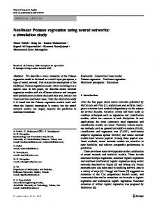
Historical perspective: back to 1957
(Prof. Pascal Vincent)
(Rosenblatt, “Perceptron”)
Machine Learning from linear regression to Neural Networks
Computer Science
Artificial Intelligence Symbolic A.I. ) ks ism or n w io t
x ne neeural n o n
Introduce machine-learning and neural networks (terminology)
C
tifi (ar
Start with simple statistical models
l
cia
Neuroscience
Feed Forward Neural Networks (specifically Multilayer Perceptrons)
Opimization + Control theory
Computer Science
Information theory
Statistics
Artificial Intelligence
rks
Statis
Physics
pu
com
Neuroscience
n
{
test point:
targets:
“horse”
inputs:
x
(1)
“cat” preprocessing, feature extraction
etc...
d
X
targets:
(feature vector)
t
(3.5, -2, ... , 127, 0, ...)
+1
(-9.2, 32, ... , 24, 1, ...)
-1
t(1)
etc... (n)
x2
“horse”
?
x(n)
x= X
{
sics tical Phy
two al ne
e neur ienc & rosc u e n nal tatio
cial artifi
inputs:
Number of examples
Symbolic A.I.
Machine Learning
Training Set
Dimensionality of input
{
Nowadays vision of the founding disciplines
(6.8, 54, ... , 17, -3, ...)
(5.7, -27, ... , 64, 0, ...)
+1
t(n)
?
Machine learning tasks
predicting t from x
Supervised learning = predict target t from input x t represents a category or “class”
• !classification (binary or multiclass)
input x ∈ IRd
n examples
the distribution of x • model !density estimation
x1 0.32 -0.12 0.06 0.91 ...
x2 -0.27 0.42 0.35 -0.72 ...
x3 +1 -1 -1 +1 ...
x4 0 1 1 0 ...
• A form for parameterized function fθ
L(fθ (x(i) ), t(i) ) i.e. overall loss over the training set
i=1
Learning amounts to finding optimal parameters:
θ
!
ˆ θ , Dn ) = arg min R(f θ
fθ x1 -0.12
: parameters
x20.42 x3-1 x14 0.22 x5
input x
t 34 target
Linear Regression
A simple learning algorithm We choose A linear mapping:
fθ (x) = !w, x" + b
Squared error loss:
dot product
with parameters: θ = {w, b}, w ∈ IRd , b ∈ IR weight vector
{
n !
y = fθ (x)
{
We then define the empirical risk as:
output
t 113 34 56 77 ...
{
• A specific loss function L(y, t)
loss function: L(y, t)
{
We need to specify:
x5 0.82 0.22 -0.37 -0.63 ...
Training Set Dn
underlying structure in x • capture ! dimensionality reduction, clustering, etc...
Empirical risk minimization
{
Unsupervised learning: no explicit target t
ˆ θ , Dn ) = R(f
target t
{
a real value • t!isregression
Learning a parameterized function fθ that minimizes a loss.
The task
bias
L(y, t) = (y − t)2 We search the parameters that minimize the overall loss over the training set ˆ θ , Dn ) θ! = arg min R(f θ
Simple linear algebra yields an analytical solution.
Linear Regression Neural network view Inuitive understanding of the dot product: each component of x weighs differently on the response.
y = fθ (x) = w1 x1 + w2 x2 + . . . + wd xd + b
A w rrow ar s r e “ ep syn re ap sen tic t “ we syn igh ap ts” tic
co n
ne c
tio
ns ”
Neural network terminology:
w1 w2
y output
linear output neuron
w5 w3 w4
b
x1 x2 x3 x4 x5
1 layer of input neurons
input x
Regularized empirical risk It may be necessary to induce a preference for some values of the parameters over others to avoid “overfitting”
We can define the regularized empirical risk as: =
#
L(fθ (x(i) ), t(i) )
+ λΩ(θ)
{
ˆ λ (fθ , Dn ) R
! n "
{
i=1
regularization term
empirical risk
Ω penalizes more or less certain parameter values λ ≥ 0 controls the amount of regularization
Ridge Regression = Linear regression + L2 regularization We penalize large weights: Ω(θ) = Ω(w, b) =!w! = 2
d !
wj2
j=1
In neural network terminology: “weight decay” penalty Again, simple linear algebra yields an analytical solution.
´ Reseaux de neurones Logistic Regression
Logistic Regression Neural network view
t ∈ {0, 1}
If we have a binary classification task:
(t = 1|x) reseaux We want to estimate conditional probability: y ! Pdes ´ La puissance expressive de neurones y ∈ [0, 1]
Sigmoid can be viewed as:
We choose
A non-linear mapping:
{
fθ (x) = fw,b (x) = sigmoid( !w, x" + b) non-linearity
logistic
sigmoid(x) =
w5
b
x1 x2 x3 x4 x5
No analytical solution, but optimization is convex
x1
decision boundary (hyperplane) mistakes
y1
y2
layer of input neurons
y3
How to obtain non-linear decision boundaries ?
Limitations of Logistic Regression y1
1
input x
z1
y2
x2
simplified model of “firing rate” response in biological neurons.
w w2 w3 4
Cross-entropy loss:
blue decision region
•
Sigmoid output neuron
x2
z1
The logistic sigmoid is the inverse of the logit “link function” in the terminology of Geleralized Linear Models (GLMs).
x2
“soft” differentiable alternative to the step function of original Perceptron (Rosenblatt 1957).
y
1 1 + e−x
L(y, t) = t ln(y) + (1 − t) ln(1 − y)
•
yAn 3
y4 old technique...
y4
• map x non-linearly to feature space: ˜ = φ(x) x
x1
Only yields “linear” decision boundary: a hyperplane
• find separating hyperplane in new space • hyperplane in new space corresponds to
red decision region
non-linear decision surface in initial x space.
! inappropriate if classes not linearly separable x1
(as on the figure) mistakes
x1
x2
x1 • exemple: y = x2 !x1x2
12
Ex. using fixed mapping
x2
x˜y =
How to obtain non-linear decision boundaries...
˜ x
) (
y3
˜y2 x
x1 x2 x2 1 αx
ˆ1 wR
Three ways to map x to x˜ = φ(x)
ˆH ˆ
R2 x1
˜y1 x
x2
R1
R1
R2
´ Reseaux de neurones
•
Use an explicit fixed mapping !previous example
•
Use an implicit fixed mapping !Kernel Methods (SVMs, Kernel Logistic Regression
•
Learn a parameterized mapping: ! Multilayer feed-forward Neural Networks such as Multilayer Perceptrons (MLP)
6
x1
´ Reseaux de neurones
NeuraldesNetwork: ´ • La puissance expressive reseaux de neurones Multi-Layer Perceptron (MLP) with one hidden layer of size 4 neurons
x2
nodeux hidden layer couches output
˜y2 x
7
Expressive power of Neural Networks with des onereseaux ´ hidden • La puissance expressive de layer neurones
x2
yz1
...)
y
x1
z1
R1
˜y3 x
x1
== Logistic regression limited to representing a separating hyperplane R2
x2
x1
˜y1 x ˜y1 x
˜y2 x
˜y3 x
˜y4 x
x2
˜y4 x
hidden ! layer x ˜ ∈ IRd
one trois hiddencouches layer ...
d
x1
x2
intput layer x ∈ IR
x1
Universal approximation property
R1
x2
R2 R2 R1
Any continuous function can be approximated arbitarily well (with a
growing number of hidden unis)
x1
´ Fonctions discriminantes lineaires Training Neural Networks
Neural Network (MLP)
We need to optimize the network’s parameters:
with one hidden layer of size d’ neurons
θ
Functional form (parametric): ˜ " + b) y = fθ (x) = sigmoid (!w, x {
{
{
d! × d
d! × 1
• •
Either batch gradient descent:
{ #
L(fθ (x ), t ) (i)
(i)
+ λΩ(θ)
regularization term (weight decay)
J(a)
aθ2
REPEAT: Pick i in 1...n
θ ←θ−η
∂ ∂θ
!
L(fθ (x(i) ), t(i) ) +
Or other gradient descent technique
" λ Ω(θ) n
aθ1
(conjugate gradient, Newton, steps natural gradient, ...)
{
i=1
{
! n "
ˆ
Rλ θ ← θ − η ∂∂θ
Or stochastic gradient descent:
ˆ λ (fθ , Dn ) = arg min R θ
ˆλ R
Initialize parameters at random Perform gradient descent REPEAT:
Optimizing parameters on training set (training the network):
θ!
ˆ λ (fθ , Dn ) = arg min R θ
˜ = sigmoid(Whidden x + bhidden ) x
Parameters: θ = {Whidden , bhidden , w, b}
• Descente de Newton
!
empirical risk
Hyper-parameters controlling capacity ! Network has a set of parameters: θ
Hyper-parameter tuning D= (x
(1)
,t
(1)
)
(x(2) , t(2) )
! optimized on the training set using gradient descent.
• • •
number of hidden units d’ regularizaiton control λ (weight decay) early stopping of the optimization
...
! There are also hyper-parameters that control model “capacity”
! tuned by a model selection procedure, not on training set. (x(N ) , t(N ) )
Divide available dataset in three
}
}
}
Training set (size n)
For each considered values of hyper-parameters: 1) Train the model, i.e. find the value of the parameters that optimize the regularized empirical risk on the training set. 2) Evaluate performance on validation set based on criterion we truly care about.
Validation set (size n’)
Test set (Size m)
Keep value of hyper-parameters with best performance on validation set.
(possibly retrain on union of train and validation ).
Evaluate generalization performance on separate test-set never used during training or validation (i.e. unbiased “out-of-sample” evaluation).
If too few examples, use k-fold cross-validation or leave-one-out (“jack-knife”)
Hyper-parameter tuning performance (error) on training set Erreur d’apprentissage performance (error) on validation set Erreur de validation
Summary •
Feed-forward Neural Networks (such as Multilayer Perceptrons MLPs) are parameterized non-linear functions or “Generalized non-linear models”...
• •
...trained using gradient descent techniques
•
Data must be preprocessed into suitable format
10,0
7,5
5,0
2,5
0 1
3
5
7
9
11
hyper-parameter value yielding smallest error on validation set is 5 (whereas it’s 1 on the training set)
13
15
Architectural details and capacity-control hyperparameters must be tuned with proper model selection procedure. standardization for continuous variable: use x−µ σ one-hot encoding for categorical variables ex: [ 0, 0, 1, 0 ]
Value of hyper-parameter
Note: there are many other types of Neural Nets...
Advantages of Neural Networks
Neural Networks
Why they matter for data mining
!The power of learnt non-linearity:
automatically extracting the necessary features
!Flexibility: they can be used for advantages of Neural Networks for data-mining. motivating research on learning deep networks.
• • • • • •
binary classification multiclass classification regression conditional density modeling
(NNet trained to output parameters of distribution of t as a function of x)
dimensionality reduction ... very adaptable framework (some would say too much...)
verview ome methods
orks
er,
Ex: using a Neural Net for dimensionality reduciton
(continued)
The classical auto-encoder framework learning a lower-dimensional representation
!Neural Networks scale well xD
zM
outputs
inputs
x1
xD
z1
Data-mining often deals with huge databases Stochastic gradient descent can handle these Many more modern machine-learning techniques have big scaling issues (e.g. SVMs and other Kernel methods)
!local minima: solution
NOT YET ayers, provides a methodIDIOT PROOF !
• • •
x1
toassociative Why then have they gone (hidden layer out of fashion in machine learning ? essedTricky versions of to train (many hyper- • Non-convex optimization • parameters to tune)
ear
Advantages of Neural Networks
depends on where you start...
Train your Neural Net
But convexity may be too restrictive. Convex problems are mathematically nice and easier, but real-world hard problems may require non-convex models.
Example of a deep architecture made of multiple layers, solving complex problems...
The promises of learning deep architectures • •
Representational power of functional composition. Shallow architectures (NNets with one hidden layer, SVMs, boosting, ...)
can be universal approximators...
•
But may require exponentially more nodes than corresponding deep architectures (see Bengio 2007).
•
! statistically more efficient to learn small deep architectures (fewer parameters) than fat shallow architectures.
The notion of
Level of Representation