Machine recognition of timbre using steady-state tone of acoustic musical instruments Ichiro Fujinaga Peabody Conservatory of Music Johns Hopkins University Baltimore, MD USA 21202
[email protected] Recent experiments indicate that steady-state portion of an acoustic musical instrument may be sufficient for timbre recognition. Here a computer-based classifier was used to recognize very short samples of steady-state tones. Gregory Sandell’s SHARC database consisted of 39 different timbre (23 orchestral instruments, some with different articulations) played at different pitches (total of 1338 spectra) were used as the samples for an exemplar-based learning system that incorporates k-nearest neighbor classifier with genetic algorithm. The latter is used to find the optimal set of weights for the features to improve the classification. The features calculated from the spectral data of the steady-state portion of the instrumental sound included centroid and other moments, such as skewness and kurtosis. As expected the centroid alone was the best single feature with a recognition rate of 20%, which is much better than chance (2.5%). The best results were obtained using seven features: the fundamental, the integral of the spectrum, the centroid, the standard deviation, the skewness, and the first two harmonic partials. What was surprising was that the recognition varied greatly between instruments. While the French horn and the muted trumpet were recognized over 90%, the recognition of other instruments, such as the cello with martele (18%), and the violin pizzicato (14%) were very poor. The average overall was 50.3%.
Introduction A timbre recognition experiment to classify 39 different orchestral instrument timbres was conducted using an exemplar-based learning system. The data consisted of the steady-state spectrum of each of the instruments played at different pitches (Sandell 1994). It has been shown that the attack portion of a musical instrument is important for identification tasks. Yet other studies show that steady-state portion is also significant (Grey 1978; Kendall and Carterette 1986). In addition to the spectral data, the moments of the spectrum, including the centroid, were considered as potential features for the identification process. The implementation of the identification task is based on a combination of a k-nearest neighbor (k-NN) classifier and a genetic algorithm, which is used for feature selection and feature weighting. This paradigm, also known as the exemplar-based learning model (Aha 1997), is attractive because training is not necessary, learning is extremely fast, algorithms are simple and intuitive, rules are not sought, and learning is incremental. The major drawback has been the high memory requirement since all examples must be stored, but the recent decrease in memory cost makes this model quite feasible. Exemplar-based model The exemplar-based learning model, analogous to “learning by examples,” is based on the idea that objects are categorized by their similarity to one or more stored examples. This model differs both from rule-based or prototypebased models of concept formation in that it assumes no abstraction or generalizations of concepts (Nosofsky 1984; 1986). The models have been successfully applied in many pattern recognition and classification tasks recognition (e.g. Fujinaga, Pennycook, and Alphonce 1989; Cost and Salzberg 1993; Fujinaga 1996). Furthermore, cognitive psychologists have found this model evident in human learning (Medin and Schaffer 1978). K-nearest-neighbor classifier The exemplar-based model can be implemented by k-NN classifier (Cover and Hart 1967), which is a classification scheme to determine the class of a given sample by its feature vector. Distances between feature vectors of an unclassified sample and previously classified samples are calculated. The class represented by the majority of knearest neighbors is then assigned to the unclassified sample. Besides its simplicity and intuitive appeal, the classifier can be easily modified, by continually adding new samples that it “encounters” into the database, to become an incremental learning system. In fact, “the nearest neighbor algorithm is one of the simplest learning methods known, and yet no other algorithm has been shown to outperform it consistently” (Cost and Salzberg 1993, 76). The standard leave-one-out procedure was used to measure the performance of the system. Moments and other features The method of moments is a versatile tool for decomposing arbitrary shape into a finite set of character features. In general, moments describe numeric quantities at some distance from a reference point or axis. Moments are
commonly used in statistics to characterize the random variable distribution and in mechanics to characterize bodies by spatial distribution mass. Here, the spectral shape is considered to be a density distribution function. Moments have a very interesting property in that the infinite sets of moments uniquely determine a function and vice versa. What this means is that any shape can be completely described by an infinite series of numbers. In practice, the loworder moments tend to describe more global shape characteristics than higher-order moments which tend to be noisy. The features used in this experiment were: the mass or the integral of the curve (zeroth-order moment), the centroid (first-order moment), the standard deviation (square root of the second-order central moment), the skewness (thirdorder central moment), kurtosis (fourth-order central moment, higher-order central moments (up to tenth), the fundamental frequency, and the amplitudes of the harmonic partials, which resulted in hundreds of features. Feature selection Feature selection involves deciding which subset of features best distinguishes among the various object types. The procedure of selecting “good” features is not formalized. Cover and Van Campenhout (1977) rigorously showed that in determining the best feature subset of size m out of n features, one needs to examine all possible subsets of size m. For practical consideration, some non-exhaustive feature selection methods must be employed. The current system implements genetic algorithms for feature selection to make the process near optimal and efficient. Genetic algorithms (GA) Genetic algorithms (Holland 1975) are often used whenever exhaustive search of the solution space is impossible or prohibitive, and are based on computational models of the evolution of individual structures via processes of selection and reproduction. The algorithm maintains a population of individuals that evolve according to specific rules of selection and other operators, such as crossover and mutation. Each individual in the population receives a measure of its fitness in the environment. Selection focuses attention on high-fitness individuals, thus exploiting the available fitness information. Since the individual’s genetic information (chromosomes) is represented as arrays of binary data, simple bit manipulations allow the implementation of mutation and crossover operations. For the feature selection, the set of features is converted to “genes,” where each feature is represented by a bit in the binary array. Therefore, each gene, having a different sequence of bits represents a subset of features to be used for classification and those having high recognition rates are made to survive in this pseudo-biological environment. Feature weights In addition to selecting a good set of features, the k-NN classifiers can be further enhanced by modifying the feature space, or equivalently, changing the weights in the distance measure (Kelly and Davis 1991). A commonly-used weighted-Euclidean metric between two vectors X and Y in an N-dimensional feature space is defined as:
N d = ∑ i =1
i
( xi − yi )
1/2
2
.
By changing the weights, i , the shape of the feature space can be changed. The feature selection is a trivial case of feature weighting where i is binary. Although feature weighting is a complex problem (Cash and Hatamian 1987), it can markedly improve the recognition rate and can also provide insights into the relative importance of each feature. Thus, the optimal use of features involves not only choosing the correct subset of the features, but also determining how much of each feature should contribute to the final decision. In feature selection, the goal was to find a set of binary weights for the features (0 or 1), but the problem now is to determine the weights that can be any real numbers. Since no known deterministic method for finding the optimal solution exits, GA is again a useful tool for finding the near-optimal set of weights from this infinite possibility (Wettschereck, Aha, and Mohri 1997). Data The data used in this experiment was based on Gregory Sandell’s SHARC database (Sandell 1994) consisted of 39 different timbre from 23 orchestral instruments, some with different articulations (see the left columns of Fig. 1 for the complete list) played at different pitches (total of 1338 spectra). For each analyzed note, Sandell’s objective was to locate a short portion of the tone that was maximally “representative” of the steady portion of the tone. Each analysis consists of a list of amplitudes and phases for all the note’s harmonics up to 10 kHz (maximum of 340 harmonics). The length of each sample was four periods of the fundamental. The source of the musical notes was the orchestral tones from the McGill University Master Samples, which are digital recordings of live musical performers.
1 2 3 4 5 6 7 8 9101112131415161718192021222324252627282930313233343536373839 1 2 3 4 5 6 7 8 9 10 11 12 13 14 15 16 17 18 19 20 21 22 23 24 25 26 27 28 29 30 31 32 33 34 35 36 37 38 39
bassfl altofl flute piccolo cbasson bsn EHorn oboe cbcl bcl Bb cl Eb cl FH FHmute tuba basstmb altotmb tmb tmbmute Bachtp C tp C tpmute CB CB mart CB mute CB pizz vlc mart vlc mute vlc pizz vlc vla mart vla mute vla pizz vla vln mart vln mute vln pizz vln vln ens
Figure 1.
26 30 37 30 32 32 30 32 23 25 37 32 37 37 31 25 13 36 33 32 34 31 38 37 39 41 44 34 39 44 36 39 34 39 34 42 37 42 44
69 0 0 0 0 0 0 0 0 0 0 0 0 0 4 0 0 0 0 0 0 0 0 0 0 0 015 4 0 0 0 4 0 0 4 0 83 10 0 0 0 7 0 0 0 0 0 0 0 0 0 0 0 0 0 0 0 0 0 0 0 0 0 0 0 0 0 0 0 0 0 011 70 5 0 0 0 0 0 0 0 0 0 0 0 0 0 8 3 0 0 0 0 0 0 0 0 0 0 0 3 0 0 0 0 0 0 0 7 50 0 0 3 0 0 0 310 0 0 0 0 0 0 0 3 7 0 0 0 0 0 0 0 0 7 0 0 0 3 0 7 6 6 0 0 59 16 0 0 0 0 0 0 0 0 0 0 0 0 0 0 0 0 3 0 0 0 3 3 0 0 0 0 0 0 0 3 3 0 3 0 9 78 0 0 0 0 0 0 0 0 0 0 0 0 3 0 0 0 0 0 0 0 0 0 0 0 3 0 0 0 0 0 017 3 0 0 0 63 0 0 0 0 0 0 0 0 0 0 0 0 0 0 0 0 3 0 0 3 0 0 3 0 0 0 0 0 3 0 0 0 3 0 016 44 0 0 3 3 0 6 0 0 6 0 0 3 6 0 0 0 0 0 0 0 0 0 0 0 3 0 0 0 0 0 0 0 4 4 0 0 78 9 0 0 0 0 0 0 0 0 0 0 0 0 0 4 0 0 0 0 0 0 0 0 0 0 0 0 0 0 0 0 0 0 0 0 0 88 012 0 0 0 0 0 0 0 0 0 0 0 0 0 0 0 0 0 0 0 0 0 0 0 0 0 0 0 0 0 0 011 0 0 68 5 0 0 0 0 0 0 3 5 3 0 0 3 0 0 0 0 0 0 0 0 0 0 0 0 0 3 0 3 0 0 3 3 0 919 50 0 0 0 0 0 0 0 0 3 0 0 0 0 0 0 0 0 0 0 0 0 0 0 3 0 0 0 0 0 0 0 0 0 0 0 0 92 0 0 3 0 3 0 0 0 0 0 0 0 0 0 0 0 0 0 0 3 0 0 0 0 0 0 0 0 0 0 0 0 0 0 0 0 97 0 3 0 0 0 0 0 0 0 0 0 0 0 0 0 0 0 0 0 0 0 0 0 0 0 0 3 0 0 0 0 0 0 0 0 0 87 0 0 0 0 0 0 0 0 0 0 3 0 0 6 0 0 0 0 0 0 0 0 0 0 0 0 0 0 0 0 0 0 0 4 0 0 72 024 0 0 0 0 0 0 0 0 0 0 0 0 0 0 0 0 0 0 0 0 8 0 0 0 0 8 0 0 0 0 015 0 0 46 0 0 0 8 0 0 0 0 0 0 0 0 0 0 0 0 0 8 0 0 014 0 0 0 0 0 0 0 0 0 3 0 0 8 6 69 0 0 0 0 0 0 0 0 0 0 0 0 0 0 0 0 0 0 3 3 6 0 0 9 0 0 0 0 6 0 0 0 0 0 0 3 64 0 0 0 0 0 0 0 0 0 0 0 3 0 0 0 0 0 0 0 0 6 0 0 0 0 0 0 3 0 0 0 0 0 0 0 0 56 16 0 0 0 0 0 0 0 0 0 0 0 3 3 0 0 0 0 6 3 0 0 0 9 0 012 0 0 0 0 0 3 0 0 9 44 0 0 0 0 0 3 0 0 0 0 0 0 9 0 0 0 0 0 0 0 0 0 0 0 0 0 0 0 0 0 0 0 0 0 0 0 91 0 0 0 0 0 0 0 0 0 6 0 3 0 0 5 0 0 016 0 3 0 5 3 0 0 0 0 0 0 0 0 3 0 0 0 37 316 0 3 8 0 0 0 0 0 0 0 0 5 0 0 0 3 0 0 0 0 0 0 0 0 0 3 0 0 0 0 0 0 0 5 51 816 3 3 0 3 0 0 0 0 0 0 5 3 0 0 8 0 0 0 0 3 0 0 0 0 0 0 0 0 0 0 0 02613 26 3 0 3 0 8 3 3 0 0 0 0 12 0 0 0 0 2 0 0 0 0 0 0 0 0 2 0 0 0 0 0 0 0 212 5 39 0 515 0 0 0 5 0 0 0 2 0 0 2 2 2 2 5 0 2 2 0 0 0 0 0 0 0 2 2 0 0 9 2 7 0 18 5 018 0 0 0 9 0 2 9 0 0 015 3 0 0 0 0 0 6 0 0 0 0 0 0 0 0 0 015 9 3 0 0 29 0 3 0 6 0 0 0 3 3 0 5 0 0 0 0 0 0 0 0 0 0 015 0 3 3 3 0 0 0 0 0 310 0 0 49 3 0 0 0 0 0 0 0 0 0 5 0 2 0 2 0 2 0 5 0 0 0 0 0 0 2 0 7 0 9 7 2 011 0 2 23 2 2 2 5 0 0 011 8 3 0 0 614 0 0 3 3 0 0 0 0 0 0 8 3 3 0 0 0 3 0 3 0 0 0 19 3 0 0 8 0 0 3 0 0 0 0 3 3 0 5 0 3 0 0 0 0 0 0 3 3 0 0 0 3 3 0 5 0 0 5 0 44 010 3 3 6 3 3 0 0 3 0 6 0 0 6 6 0 0 3 0 0 0 3 0 3 0 0 6 0 6 0 0 6 3 0 0 35 0 0 0 0 0 0 3 0 0 0 0 0 3 8 0 0 0 0 0 0 0 0 3 8 0 0 3 0 010 0 010 0 8 0 36 5 0 0 0 0 6 0 0 6 3 0 0 0 0 0 0 0 0 3 0 0 6 9 0 0 0 0 0 3 3 0 0 612 021 15 3 2 2 010 0 0 0 2 0 0 0 2 0 0 0 0 0 0 0 0 0 0 5 0 7 0 2 2 0 0 0 5 2 2 0 50 3 311 3 0 3 3 3 0 0 0 3 3 0 0 0 3 0 8 3 3 0 0 3 0 0 0 0 8 014 011 0 0 3 0 0 010 0 0 0 5 0 2 0 0 0 0 0 0 2 0 0 5 0 0 0 0 0 0 0 0 0 5 014 012 214 2 0 016 0 0 2 5 0 0 2 7 0 0 0 0 0 0 0 5 0 0 0 2 2 0 7 0 0 2 0 2 011 2 0
0 0 0 0 0 0 0 0 0 0 0 0 0 0 0 0 0 0 0 0 3 0 3 3 0 0 0 0 0 0 0 3 0 0 0 3 0 0 0 0 0 0 0 0 0 0 0 0 8 0 0 0 0 0 3 0 0 0 9 3 0 3 0 0 0 0 0 0 0 0 0 0 0 0 0 0 0 0 0 2 2 0 0 0 5 0 0 0 7 2 3 0 0 0 3 3 0 0 3 0 5 0 0 6 0 0 2 2 8 0 5 0 21 7 2 9 20
Recognition rate (%) for each instrumental timbre with 7 features. The first column right of the name indicates the number of pitches in each timbre. Average was 50.3%. wt = {0.25, 0.25, 0.94, 0.62, 0.31, 0.19, 0.25}, k=5
Timbre recognition The initial analysis showed that, as expected, the centroid alone was the best single feature with the recognition rate of 20% (k=57), which is much better than chance (2.5%). When the GA was used for feature selection, i.e. finding the subset of 352 features that results in the best recognition score, the optimal results were obtained using seven features: the fundamental, the integral of the spectrum, the centroid, the standard deviation, the skewness, and the first two harmonics. The further application of GA resulted in the feature weights of {0.25, 0.25, 0.94, 0.62, 0.31, 0.19, 0.25}. The complete result is shown in Figure 1. What was surprising was that the recognition varied greatly between instruments. While the French horn and the muted trumpet were recognized over 90%, the recognition of other instruments, such as the violin with martele (15%) and the violin pizzicato (8%) were very poor. The average overall was 50% (k=5). Using only four features (fundamental, centroid, standard deviation, and skewness) the system scored 42% (k=3). These results are similar to human subject identification performance. In the experiment by Saldanha and Corso (1964), the subjects, who coincidentally had 39 possible instruments to choose from, identified recorded sounds of ten orchestral instruments with the average of 39%. Interestingly, as in this study, the accuracy varied widely, ranging from 9% to 84%. The subjects in the Kendall’s (1986) experiment had three instruments to choose from and the results using the same instruments are shown in Figure 2, which are comparable to Kendall’s results. Conclusions Using exemplar-based learning model, the computer was able to identify orchestral instruments comparable to human performance using a very few features. This was achieved using a spectrum of very short steady-state portions of the instrumental sound recorded at different pitches. To improve the recognition rate, other features may be incorporated, such as attack transients (spectral flux), linear spectral irregularity (Kendall 1996), mel-frequency cepstrum coefficients (De Poli and Prandoni 1997), cortical representation (Ru and Shamma 1997), and polyspectra (Dubnov et al. 1997).
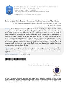
1 2 3
Bb cl C tp vln
37 34 42
1
2
3
84 9 17
14 79 5
3 12 79
1 2 3
Bb cl C tp vln
37 34 42
1
2
3
62 15 7
24 74 24
14 12 69
Figure 2a. Recognition rate (%) for three instrumental Figure 2b. Recognition rate (%) for three instrumental timbre with 7 features. Average was 80.5%. timbres with 4 features. Average was 68.1% wt = {0.50, 0.06, 0.94, 0.50, 0.44, 0.25, wt={0.29, 1.00, 0.48, 0.25}, k=1 0.25}, k=3
Bibliography Aha, D. W. 1997. Lazy learning. Artificial Intelligence Review 11 (1–5): 7–10. Berger, K. W. 1964. Some factors in the recognition of timbre. Journal of the Acoustical Society of America. 36 (10): 1888–91. Cash, G. L., and M. Hatamian. 1987. Optical character recognition by the method of moments. Computer Vision, Graphics, and Image Processing 39 (3): 291–310. Cost, S., and S. Salzberg. 1993. A weighted nearest neighbor algorithm for learning with symbolic features. Machine Learning 10: 57–78. Cover, T., and P. Hart. 1967. Nearest neighbor pattern classification. IEEE Transactions on Information Theory 13 (1): 21–7. Cover, T. M., and J. M. Van Campenhout. 1977. On the possible orderings in the measurement selection problem. Transactions on Systems, Man, and Cybernetics 7 (9): 657–61. De Poli, G., and P. Prandoni. 1997. Sonological models for timbre characterization. Journal of New Music Research. 26 (2): 170–97. Dubnov, S., N. Tishby, and D. Cohen. 1997. Polyspectra as measures of sound texture and timbre. Journal of New Music Research. 26 (4): 277–314. Fujinaga, I. 1996. Exemplar-based learning in adaptive optical music recognition system. Proceedings of the International Computer Music Conference. 55–6. Fujinaga, I., B. Pennycook, and B. Alphonce. 1989. Computer recognition of musical notation. Proceedings to the First International Conference on Music Perception and Cognition. 87–90. Grey, J. M. 1987. Timbre discrimination in musical patterns. Journal of the Acoustical Society of America. 64 (2): 467–72. Holland, J. H. 1975. Adaptation in natural and artificial systems. Ann Arbor: U. of Michigan Press. Kelly, J. D., and L. Davis. 1991. Hybridizing the genetic algorithm and the k nearest neighbors classification algorithm. Fourth International Conference on Genetic Algorithms and their Applications. 377–83. Kendall, R. A. 1986. The role of acoustic signal partitions in listener categorization of musical phrases. Music Perception. 4 (2): 185–214. Kendall, R. A., and E. C. Carterette. 1996. Difference thresholds for timbre related to spectral centroid. Proceedings of the Fourth International Conference on Music Perception and Cognition. 91–5. Medin, D. L., and M. M. Schaffer. 1978. Context theory of classification learning. Psychological Review 85: 207–38. Nosofsky, R. M. 1986. Attention, similarity, and the identification categorization relationship. Journal of Experimental Psychology: General 115 (1): 39–57. Nosofsky, R. M. 1984. Choice, similarity, and the context theory of classification. Journal of Experimental Psychology: Learning, Memory, and Cognition 10 (1): 104–14. Ru, P, and S. A. Shamma. 1997. Representation of musical timbre in the auditory cortex. Journal of New Music Research. 26 (2): 154–69. Saldanha, E. L., and J. F. Corso. 1964. Timbre cues and the identification of musical instruments. Journal of the Acoustical Society of America. 36(11): 2021–6. Sandell, G. J. 1994. SHARC timbre database. http://www.parmly.luc.edu/sharc. Siedlecki, W. S., J. 1989. A note on genetic algorithms for large-scale feature selection. Pattern Recognition Letters 10 (5): 335–47. Wettschereck, D., D. W. Aha, and T. Mohri. 1997. A review and empirical evaluation of feature weighting methods for a class of lazy learning algorithms. Artificial Intelligence Review 11 (1–5): 272–314.