Jul 15, 2010 - Patrick Dular1,2, Ruth V. Sabariego1, Laurent Krähenbühl3, Christophe Geuzaine1. 1 University of Liège, Dept. of Electrical Engineering and ...
Author manuscript, published in "SCEE, Toulouse : France (2010)"
Magnetic model refinement via a coupling of finite element subproblems Patrick Dular1,2, Ruth V. Sabariego1, Laurent Krähenbühl3, Christophe Geuzaine1 1 2 3
University of Liège, Dept. of Electrical Engineering and Computer Science, ACE, B-4000 Liège, Belgium F.R.S.-FNRS, Fonds de la Recherche Scientifique, Belgium Université de Lyon, Ampère (UMR CNRS 5005), École Centrale de Lyon, F-69134 Écully Cedex, France
Summary. Model refinements of magnetic circuits are performed via a subdomain finite element method. A complete problem is split into subproblems with overlapping meshes, to allow a progression from source to reaction fields, ideal to real flux tubes, 1-D to 3-D models, perfect to real materials, statics to dynamics, with any coupling of these changes. Its solution is then the sum of the subproblem solutions. The procedure simplifies both meshing and solving processes, and quantifies the gain given by each refinement on both local fields and global quantities.
hal-00502627, version 1 - 15 Jul 2010
1 Introduction The perturbation of finite element (FE) solutions provides clear advantages in repetitive analyses and helps improving the solution accuracy [1-6]. It allows to benefit from previous computations instead of starting a new complete FE solution for any geometrical, physical or model variation. It also allows different problem-adapted meshes and computational efficiency due to the reduced size of each subproblem. A general framework allowing a wide variety of refinements is herein developed. It is defined as a subproblem FE approach based on canonical magnetostatic and magnetodynamic problems solved in a sequence, with at each step volume sources (VSs) and surface sources (SSs) originated from previous solutions. VSs express changes of material properties. SSs express changes of boundary conditions (BCs) or interface conditions (ICs). Common and useful changes from source to reaction fields, ideal to real flux tubes (with leakage flux), 1-D to 3-D models, perfect to real materials, and statics to dynamics, can all be defined through combinations of VSs and SSs. The developments are performed for the magnetic vector potential FE formulation, paying special attention to the proper discretization of the constraints involved in each subproblem. The method will be illustrated and validated on various problems.
2. Series of Coupled Subproblems Instead of solving a complete problem, with all its details, it is proposed to split it into a sequence of subproblems, some with approximated geometrical or physical data, including model simplifications, and others performing adequate corrections. The complete solution is then the sum of the subproblem solutions. This offers a way to perform model refinements, with a direct access to each correction, usually of useful physical meaning.
Each subproblem is defined in its own domain, generally distinct from the complete one. At the discrete level, this aims to decrease the problem complexity and to allow distinct meshes with suitable refinements. Each subproblem approximates at best its contribution to the complete solution. The domains of the subproblems usually overlap. Each subproblem p is defined in a domain Ωp, with boundary ∂Ωp = Γp. It is governed by magnetostatic or magnetodynamic equations and constrained with VSs and SSs, of which some components originate from previous problems q. The involved fields are the magnetic field hp, the magnetic flux density bp and the electric field ep. Classical VSs fix remnant inductions in magnetic materials and current densities in stranded inductors. Similar VSs can also express changes of permeability µ and conductivity σ from a problem q to a problem p [4, 5]. For changes from µq to µp and from σq to σp, the magnetic and electric material relations for problem p are hp = µp–1 bp + hs,p and jp = σp ep + js,p, with VSs hs,p = (µp–1 – µq–1) bq and js,p = (σp – σq) eq limited to the modified regions. The usually homogeneous SSs, i.e. BCs or ICs for the traces n × hp|γp, n ⋅ bp|γp and n × ep|γp, with n the unit exterior normal and γp ⊂ Γp, can be extended to non-zero constraints. The resulting ICs, i.e. the discontinuities [n × hp]γp = jf,p, [n ⋅ bp]γp = bf,p and [n × ep]γp = ff,p through an interface γp, involve SSs jf,p, bf,p and ff,p obtained from previous problems. Usually, free forced discontinuities in a problem q, allowing some simplifications with idealized thin regions [2-5], can be removed in a problem p via opposed SSs, i.e. jf,p = – [n × hq]γp, bf,p = – [n ⋅ bq]γp and ff,p = – [n × eq]γp (γp and γq only differ at the discrete level by their meshes). For the ICs to be defined in a weak sense, a post-treatment of the FE weak formulation is done to naturally express the SSs via a volume integration limited to a layer of FEs surrounding the interface [2-5]. VSs and SSs involve previous solutions in subdomains of the current problem p. At the discrete level, this means these solutions have to be expressed in portions of the mesh of problem p, while initially given in the mesh of problem q. This is done via an L2-projection [2-6].
3. Various Correction Procedures Various correction schemes, appropriate to practical magnetic system analyses, can benefit from the developed subproblem approach. These are summarized below and will be discussed in details.
hal-00502627, version 1 - 15 Jul 2010
(1) Change of material properties (Fig. 1) – A typical problem is that of a region put in an initially calculated source field b1. The associated subproblem 2 is solved in its proper mesh, with the added core and its surrounding region, and VSs limited to this core, where µ and/or σ are modified. Such changes can occur when adding or suppressing materials or portions of those, in, e.g., shape optimization, non-destructive testing [1, 6], moving systems. (2) Change from ideal to real flux tubes [3-4] (Fig. 2) – A problem q can first consider ideal tubes [7], i.e. surrounded by perfect flux walls through which n ⋅ bq|γq is zero and bq and hq outside are zero. The complementary trace n × hq|γq is unknown and non-zero. Consequently, a change to a permeable flux wall defines a problem p with SSs opposed to this non-zero trace. This change (2) can be done simultaneously with change (1), which is the case in Fig. 3: the leakage flux b3 completes the ideal distribution b1 while knowing the source b2 proper to the inductor; this allows independent overlapping meshes for both source and reaction fields. (3) Change from 1-D to 3-D [5] – Change (2) can be extended to allow a dimension change, e.g. from 2-D to 3-D: a 2-D solution is first considered as limited to a certain thickness in the third dimension, with a zero field outside; on the other side, another independent problem is solved. Changes of ICs on each side of this portion, via SSs, then allow the calculation of 3-D end effects. Series connections of flux tubes use a similar procedure: a violation of ICs when connecting two flux tubes can be corrected via an opposed SS, e.g. which allows changes from 1-D to 2-D (Fig. 3). (4) Change from perfect to real materials [2] (Fig. 4) – A problem q can first consider perfect conducting (resp. magnetic) materials, with σq→∞ (resp. µq→∞), in which case the trace n ⋅ bq|γq (resp. n × hq|γq) on its boundary is zero and bq (resp. hq) inside is zero. The complementary trace n × hq|γq (resp. n ⋅ bq|γq) is unknown and non-zero. Consequently, a change to a finite σp (resp. µp) defines a problem p with SSs opposed to this non-zero trace. (5) Change from statics to dynamics, to accurately render skin and proximity effects.
4.
5. 6.
7.
Method for Magnetic Model Refinement of Air Gaps and Leakage Fluxes. IEEE Trans. Magn., 45-3:1400-1403, 2009. P. Dular, R.V. Sabariego, M.V. Ferreira da Luz, P. KuoPeng, and L. Krähenbühl. Perturbation finite-element method for magnetic circuits. IET Science, Measurement & Technology, vol. 2, no. 6, pp. 440-446, 2008. P. Dular, R.V. Sabariego, and L. Krähenbühl. Magnetic Model Refinement via a Perturbation Finite Element Method – From 1-D to 3-D. COMPEL, 28-4:974-988, 2009. P. Dular and R. V. Sabariego. A perturbation method for computing field distortions due to conductive regions with hconform magnetodynamic finite element formulations. IEEE Trans. Magn., 43-4:1293-1296, 2007. C. Chillet and J.Y. Voyant. Design-oriented analytical study of a linear electromagnetic actuator by means of a reluctance network. IEEE Trans. Magn., 37-4:3004-3011, 2001.
Y Z
Y X
Z
X
Fig. 1. Field lines for an inductor alone (b1, left) and for an added core (b2, µr,core = 100) (right); distinct meshes are used for problems 1 and 2.
Y Z
Y X
Z
Y X
Z
Y X
Z
X
Fig. 2. An electromagnet: field lines in an ideal flux tube (b1, µr,core = 100), for the inductor alone (b2), for the leakage flux (b3) and for the total field (b) (left to right).
Y Z
Y X
Z
Y X
Z
X
Fig. 3. Series connection of two flux tubes: field lines in ideal flux tubes (b1, left), local correction at the junction (b2, middle) and complete solution (b, right).
Acknowledgement. This work was partly supported by the Belgian Science Policy (IAP P5/34) and the Belgian French Community (Research Concerted Action ARC 03/08-298).
X Y
X
Z
Y
Z
X Y
X
Z
Y
Z
References 1.
2.
3.
Z. Badics, Y. Matsumoto, K. Aoki, F. Nakayasu, M. Uesaka, and K. Miya. An effective 3-D finite element scheme for computing electromagnetic field distorsions due to defects in eddy-current nondestructive evaluation. IEEE Trans. Magn., 33-2:1012-1020, 1997. P. Dular, R. V. Sabariego, J. Gyselinck, and L. Krähenbühl. Sub-domain finite element method for efficiently considering strong skin and proximity effects. COMPEL, 26-4:974-985, 2007. P. Dular, R. V. Sabariego, M. V. Ferreira da Luz, P. KuoPeng, and L. Krähenbühl. Perturbation Finite Element
Z
Z Y
X
Y
X
Fig. 4. Transverse flux system (3-turn inductor above a half plate, with perpendicular flux horizontal symmetry axis below); a low (left) and a high (right) electric conductivity are considered for the plate; from top to bottom: magnetic flux lines (phase 0) for the reference solution b1 with a perfectly conductive inductor, the perturbation solution b2 and the perturbed solutions b; bottom: current density distribution (modulus).