NATCAR Magnetic Sensor Modeling by Darren Liccardo, Spring 2002. UC
Berkeley, EE192. Accurate magnetic sensing is key to building a successful
steering ...
†
NATCAR Magnetic Sensor Modeling by Darren Liccardo, Spring 2002 UC Berkeley, EE192 Accurate magnetic sensing is key to building a successful steering controller for NATCAR. This document explores the dynamics of magnetic sensing and modeling in the NATCAR Environment.
Goal We would like to detect the position of our vehicle with respect to a current carrying conductor parallel to the direction of motion. We will explore the orientations of two magnetic sensing inductors and model their response with respect to certain parameters.
System Definition Below is a system overview of our vehicle behavior. Our sensor dynamics will determine some transfer function from x to (s1,s2 ) , where x is the orthogonal distance between our vehicle and the track, and (s1,s2 ) are the output voltages of our two sensors. We must somehow combine these values (sensor fusion) to give us a meaningful error signal for our controller. Ideally, we would simply like to feed our controller x , after all, the true meaning of error is our distance away from the track.
Vehicle and Track Dynamics
x
Sensor Dynamics
s1,s2 d, t
Sensor Fusion
error Actuator Dynamics
Controller PWM ,PWM servo motor
Sensor Modeling To solve the sensor dynamics, we will model an inductor’s response to the track, as depicted below. This is drawn as if you were sitting in the vehicle, looking forward at your sensors. The following variables have been defined: Æ
I the directed current in the track Æ
B r h x a b
the magnetic field induced by the current in the track the distance between the inductor and the track the height of the inductor from the floor the horizontal distance from the inductor to the track the tilt of the inductor from the horizontal the angle to the inductor from the floor
a
Æ
B
r
h
b
x
Æ
I
We would like to solve for S(a, x,h,I) , that is, our sensor output as a function of tilt angle, height, horizontal distance, and track current.
Solving the Model
solve for S(a ,x,h ,I ) . From Electricity and Magnetism:
B=
mo I I = k1 2p r r
for a long straight wire
In reality, the B field is changing with the AC current in the track, however, we can neglect the differential notation of Faraday’s Law without changing the result. Below a proportion is written that accounts for the angle of the inductor with respect to the magnetic flux. We assume that our amplifier circuit has a constant gain k2 .
S µ Bcos(p /2 - [a + b ]) S µ Bsin(a + b) kI S = k 2 Bsin(a + b ) = sin(a + b) r kI S = (sin a cos b + cosa sin b ) r kI x h kI S = ( sin a + cos a) = 2 (x sin a + hcos a) r r r r kI S(a, x,h,I) = 2 (x sina + h cosa) 2 h +x We now have a sensor model that lets us investigate sensor response with respect to tilt angle, horizontal distance from the track, height, and track current.
†
Some Results The following results show three potential sensor responses.
S(0,x,2cm,100mA)
2 A tilt angle of 0 degrees shows a response that tails off as ~ 1/ x .
S( p / 2,x,2cm,100mA)
A tilt angle of 90 degrees has a null directly over the track, and tails off as ~ 1/ x .
S( p / 4,x,2cm,100mA)
A tilt angle of 45 degrees allows differentiation between the two sides of the track.
†
In conclusion, a tilt angle of 90 degrees gives the most dynamic range, yet produces a discontinuity directly over the track. A tilt angle of 0 degrees show a smooth and symmetric response, however, its steep slope limits its range. Finally, a tilt angle of 45 degrees can be used to detect the magnetics on one side of the track only with its highly asymmetric response.
Sensor Fusion Now that the sensor dynamics have been explored, lets look at how a two-sensor system can be fused to create an error signal. Remember, we are trying to create an error signal that is linear with the vehicle’s orthogonal distance from the track because this is the true error that we are interested in controlling. We would like to design a relation error(s1 ,s2 ). Ideally, error(s1 ,s2 ) = x . We would like this relation to be insensitive to changes in track current, and insensitive to differential gains between the two sensors. The following graph shows three potential error functions using two sensors spaced 10cm apart with responses s(0, x - 5cm,2cm,100mA) and s(0, x + 5cm,2cm,100mA).
1 0.8
errorgreen (s1 ,s2 ) =
0.6 0.4
errorred (s1 ,s2 ) =
0.2
1 1 s1 s2
s2 - s1 4.7
0 -0.2 -0.4
errorblue (s1 ,s2 ) =
1.5 1.5 s1 s2
-0.6 -0.8 -1 -15
-10
-5
0 position error (cm)
5
Both errorgreen and errorblue have reasonably linear regions.
10
15
The graph below shows the same error functions under conditions of half the nominal track current (50mA):
errorgreen maintains its gain and maintains its linearity in the presence of half the track current.
Conclusion Accurate sensor modeling and well-designed sensor fusion will help keep your NATCAR controller robust and stable under varying track conditions, and sensor orientations. I have presented a possible solution in this design space, and presented the framework for investigating other potential solutions.