Magnetometer Integrated Navigation System

Hindawi Publishing Corporation Journal of Sensors Volume 2016, Article ID 6105803, 10 pages http://dx.doi.org/10.1155/2016/6105803

Research Article Optical Flow Sensor/INS/Magnetometer Integrated Navigation System for MAV in GPS-Denied Environment Chong Shen,1 Zesen Bai,2 Huiliang Cao,1 Ke Xu,1 Chenguang Wang,1 Huaiyu Zhang,1 Ding Wang,1 Jun Tang,1 and Jun Liu1 1

National Key Laboratory for Electronic Measurement Technology, Key Laboratory of Instrumentation Science & Dynamic Measurement, Ministry of Education, School of Instrument and Electronics, North University of China, Taiyuan 030051, China 2 School of Electronics Engineering and Computer Science, Peking University, Beijing 100871, China Correspondence should be addressed to Jun Liu; [email protected] Received 19 November 2015; Accepted 12 January 2016 Academic Editor: Fadi Dornaika Copyright © 2016 Chong Shen et al. This is an open access article distributed under the Creative Commons Attribution License, which permits unrestricted use, distribution, and reproduction in any medium, provided the original work is properly cited. The drift of inertial navigation system (INS) will lead to large navigation error when a low-cost INS is used in microaerial vehicles (MAV). To overcome the above problem, an INS/optical flow/magnetometer integrated navigation scheme is proposed for GPS-denied environment in this paper. The scheme, which is based on extended Kalman filter, combines INS and optical flow information to estimate the velocity and position of MAV. The gyro, accelerator, and magnetometer information are fused together to estimate the MAV attitude when the MAV is at static state or uniformly moving state; and the gyro only is used to estimate the MAV attitude when the MAV is accelerating or decelerating. The MAV flight data is used to verify the proposed integrated navigation scheme, and the verification results show that the proposed scheme can effectively reduce the errors of navigation parameters and improve navigation precision.

1. Introduction Recently, the autonomous operating unmanned aerial vehicle (MAV) is becoming popular in military and civilian applications [1–3], such as aerial surveillance, cargo delivery, search and rescue, and remote sensing and mapping. A reliable navigation system is very important for safely operating the MAV. Currently, global positioning system (GPS) [4] and inertial navigation system (INS) [5] are the most widely used navigation techniques for the MAV. GPS is based on satellite which can provide relatively consistent accuracy navigation; however, the satellite signals would be lost in city canyon or indoor environments [6, 7]. INS is a self-contained device which can offer a complete set of navigation parameters with high frequency, including attitude, velocity, and position; however, the rapid growth of systematic errors with time is a main drawback of stand-alone INS [8, 9]. Due to the drawbacks of GPS and INS, lots of novel navigation devices have been studied. For example, optical flow sensor has been proved which can provide reliable

velocity and position information when applied for robot localization or navigation [10, 11]. Optical flow techniques are motivated by bird and insect flights which are used to solve the navigation problem. Optical flow can be thought to be the 2D projection of the 3D perceived motion of the objects, which has been widely utilized for motion estimation [12, 13]. When facing the ground, the optical flow sensors can be used for accurate velocity calculation, and the position can be obtained by integration. For example, computer mouse sensor is a successful application of optical flow theory. Benefiting from previous study of optical flow algorithm and hardware design, robotics researchers have employed optical flow sensors for the MAV navigation. Ding et al. [14] added optical flow into the GPS/INS integration for UAV navigation where optical flow rate is used as backup velocity aiding in case of GPS signal outages, and the verification results showed that, by using optical flow, the height estimation was still within a meter range within 20 seconds after GPS dropped out. Mercado et al. [15] proposed a GPS/INS/optical flow data

2

Journal of Sensors

Preceding frame

Current frame j

xc (i + Δi, j + Δj)

Δi Target block in

V Δj

xp (i, j)

current frame i

Target block

d

Optical flow vector

Search area

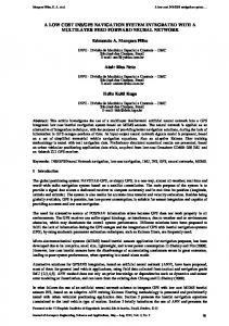
Figure 1: Block matching algorithm based on sum of absolute differences.

fusion method for position and velocity estimation; experiment results showed that a good velocity measurement could be obtained by optical flow under rough GPS conditions. Rhudy et al. [16] aided wide-field optical flow to INS for UAV, where the wide-field optical flow was used to regulate INS drift for the purpose of GPS-denied navigation. Gageik et al. [17] applied an optical flow sensor for 2D positioning of UAV, and position hold result showed that the standard deviation of the position error was just 10 cm and the position error was just about 30 cm after landing. It can be clearly seen that the optical flow is an effective solution for velocity and position measurement. However, traditional optical flow is detected by video camera, which is not suitable for MAV because of the weight, size, and power. In 2013, an optical flow sensor based on a machine vision CMOS image sensor for MAV was proposed and named as PX4FLOW [18], and the indoor verification results showed that the error was just 0.5 m with the overall trajectory being 28.44 m. Compared to traditional optical flow sensors, PX4FLOW is of low power, low latency, small size, and low cost; therefore, it is very suitable for MAV applications. In this paper, an optical flow sensor/INS/magnetometer integrated navigation system is proposed for MAV, where optical flow sensor is used to measure the velocity and position of the MAV, and the magnetometer is used to measure the attitude of the MAV; then, these navigation parameters are applied to calibrate the drift of INS by using an extend Kalman filter. This paper is organized as follows: Section 2 is the theory of velocity and position estimation by optical flow. The data fusion model is given in Section 3. Section 4 is the experiment and verification. Section 5 is the conclusion.

2. Estimation of Velocity and Position by Optical Flow Sensor 2.1. The Calculation of Optical Flow. Optical flow is the projection of 3D relative motion onto a 2D image plane. In order

to calculate the optical flow, the researchers have proposed many solutions, such as Lucas-Kanade algorithm, HornSchunck algorithm, image interpolation algorithm, block matching algorithm, and feature matching algorithm. In our study, considering the complexity of the software calculation and hardware platform, the block matching algorithm (BMA) based on minimum mean absolute error (MMAE) and the sum of absolute differences (SAD) are selected to calculate the optical flow, which is shown in Figure 1. As shown in Figure 1, 𝑥𝑝 (𝑖, 𝑗) is set as the gray value of 𝑛 × 𝑛 target block selected from the previous frame, and 𝑥𝑐 (𝑖 + Δ𝑖, 𝑗 + Δ𝑗) is the gray value of the target block which is to be matched in the searching area of current frame, where 1 ≤ 𝑖, 𝑗 ≤ 𝑛, −𝑑 ≤ Δ𝑖, Δ𝑗 ≤ 𝑑. The principle of BMA based on MMAE and the SAD is to search Δ𝑖 and Δ𝑗 which satisfy (1); then, the optical flow vector V = 𝑟(Δ𝑖, Δ𝑗)𝑇 can be obtained, where the unit of V is pixel/sec; 𝑟 is the sample frequency of the camera and the unit is fram:e/sec; 𝑈 is the minimum mean absolute error: 𝑛 𝑛 󵄨 󵄨 SAD (Δ𝑖, Δ𝑗) = ∑ ∑ 󵄨󵄨󵄨󵄨𝑥𝑐 (𝑖 + Δ𝑖, 𝑗 + Δ𝑗) − 𝑥𝑝 (𝑖, 𝑗)󵄨󵄨󵄨󵄨 , 𝑗=1𝑗=1

𝑈 = min {SAD (Δ𝑖, Δ𝑗)} , (Δ𝑖,Δ𝑗)

𝑇 󵄨󵄨 V = 𝑟 (Δ𝑖, Δ𝑗) 󵄨󵄨󵄨 . 󵄨𝑈

(1) (2) (3)

In the initial state, a target is selected at the original point of the imaging plane; the target block will move when the MAV moves. In the searching area of the current frame, the optical flow vector of the target block can be obtained by calculating the minimum SAD between the current block and the previous block. In the experiment, the images which are perpendicular to the camera are collected. In the whole collecting process, a data block which is 8 × 8 pixel is used as the block matching object, and the searching area contains ±4 pixels. So there

Journal of Sensors

3 where 𝜔 = [𝜔𝑥 , 𝜔𝑦 , 𝜔𝑧 ]𝑇 is angular velocity of MAV; Tc = [𝑇𝑥𝑐 , 𝑇𝑦𝑐 , 𝑇𝑧𝑐 ]𝑇 is average velocity of MAV under camera coordinate system. After derivation calculus to (4), the relationship between the velocity of Pc under the camera coordinate system and the velocity of p under the image plane can be obtained:

O Xc

Yc f

p (x, y, f) Zc

𝑍Vc − 𝑉𝑧 Pc flow , =k=𝑓 Δtime 𝑍𝑐2

where k = [V𝑥 , V𝑦 , V𝑧 ]𝑇 , and (10)–(12) can obtained by expanding (9):

Pc (Xc , Yc , Zc )

Figure 2: The model of pin-hole image plane.

are 64 pixel points and 81 candidate vector directions in each frame image. After obtaining each frame image, the mean absolute errors of each candidate vector are calculated and the minimum value is selected as the optical flow vector. 2.2. The Model of Optical Flow. The motion model of optical flow is projecting the three-dimensional motion onto the two-dimensional image plane of the camera. There are two common optical flow estimation models: one is pin-hole image plane approach which is derived from the principle of insect and vertebrate visual system; the other is spherical imaging surface approach which is derived from insect compound eyes. In our study, the pin-hole image plane approach is used to estimate the motion of MAV under geographic coordinate system. The pin-hole image plane model is shown as in Figure 2. Pc = [𝑋𝑐 , 𝑌𝑐 , 𝑍𝑐 ]𝑇 is set as a point under camera coordinate system; 𝑓 stands for the focal length, so Pc can be expressed as p = [𝑥, 𝑦, 𝑓]𝑇 : p=𝑓

Pc , 𝑍𝑐

(4)

𝑥=𝑓

𝑋𝑐 , 𝑍𝑐

(5)

𝑦=𝑓

𝑌𝑐 . 𝑍𝑐

(6)

Considering any point P on the ground, point P has the following relationship relative to the MAV under the camera coordinate system: Vc = −Tc − 𝜔 × Pc .

(7)

Equation (7) is expanded in three dimensions and (8) can be obtained: 𝑉𝑥𝑐 = −𝑇𝑥𝑐 − (𝜔𝑦 𝑍𝑐 − 𝜔𝑧 𝑌𝑐 ) , 𝑉𝑦𝑐 = −𝑇𝑦𝑐 − (𝜔𝑧 𝑋𝑐 − 𝜔𝑥 𝑍𝑐 ) , 𝑉𝑧𝑐 = −𝑇𝑧𝑐 − (𝜔𝑥 𝑌𝑐 − 𝜔𝑦 𝑋𝑐 ) ,

(9)

(8)

V𝑥 =

𝑓 (𝑉 𝑍 − 𝑉𝑧 𝑍𝑥 ) , 𝑍𝑐2 𝑥𝑐 𝑐

(10)

V𝑦 =

𝑓 (𝑉 𝑍 − 𝑉𝑧 𝑍𝑦 ) , 𝑍𝑐2 𝑦𝑐 𝑐

(11)

V𝑧 = 0.

(12)

Substituting (8) into (10) and (11), (13) can be obtained: V𝑥 = V𝑦 =

𝑇𝑧𝑐 𝑥 − 𝑇𝑥𝑐 𝑓 𝑍𝑐 𝑇𝑧𝑐 𝑦 − 𝑇𝑦𝑐 𝑓 𝑍𝑐

− 𝜔𝑦 𝑓 + 𝜔𝑧 𝑦 + + 𝜔𝑥 𝑓 − 𝜔𝑥 𝑦 +

𝜔𝑥 𝑥𝑦 − 𝜔𝑦 𝑥2 𝑓 𝜔𝑥 𝑦2 − 𝜔𝑦 𝑥𝑦 𝑓

, (13) .

In (13), V𝑥 and V𝑦 are the optical flow components on directions 𝑥 and 𝑦, which can be calculated by SAD and BMA. 𝑍𝑐 can be obtained by ultrasonic which was integrated in the optical flow sensor. Angular velocity 𝜔𝑥 , 𝜔𝑦 , and 𝜔𝑧 can be obtained by gyroscope; 𝑥 and 𝑦 can be substituted by (2) and (3). Therefore, the translational velocity Tc of the MAV under the camera coordinate system can be estimated, and the MAV velocity under geographic coordinate system can be calculated through coordinate transformational matrix Cnc . After integration of velocity, the data for position of MAV can be obtained at last. 2.3. Attitude Estimation Based on Accelerometer/Magnetometer. By measuring the gravitational field, the accelerometer can determine the roll and pitch of the MAV under the condition of no own acceleration; by measuring the geomagnetic field, the magnetometer can determine the heading of MAV based on the vehicle’s attitude information provided by accelerometer. Then, the whole attitude information without accumulated error can be obtained by integrating accelerometer/magnetometer. 2.3.1. The Roll and Pitch Obtained by Accelerometer. The component of gravity vector under the geographic coordi𝑇 nate system is [0 0 −𝑔] . When the vehicle is static (no relative acceleration to the navigation coordinate system), the measured value of accelerometer which is fixed in the 𝑇 carrier coordinate system is a𝑏 = [𝑎𝑥𝑏 𝑎𝑦𝑏 𝑎𝑧𝑏 ] . The heading of the vehicle has no influence on the output of

4

Journal of Sensors

accelerometers of directions 𝑥 and 𝑦 due to the gravitational acceleration perpendicular to horizontal plane. Therefore, it can be concluded that 𝑎𝑥 0 cos 𝛾 sin 𝛾 sin 𝜃 − sin 𝛾 cos 𝜃 [ 𝑏] [ ] [ [𝑎𝑦 ] = [ 0 cos 𝜃 sin 𝜃 ] [ 0 ] ] . (14) [ 𝑏] [𝑎𝑧𝑏 ] [ sin 𝛾 − cos 𝛾 sin 𝜃 cos 𝛾 cos 𝜃 ] [−𝑔] The roll and pitch can be calculated: 𝜃 = arcsin (−

𝑎𝑦𝑏

𝛾 = arctan (−

𝑔

),

𝑎𝑥𝑏 𝑎𝑧𝑏

(15) ).

This method uses the projection information of the earth’s gravitational acceleration in carrier coordinate system to reflect the attitude information of the vehicle, so the above

equations are correct only under the condition that there is no acceleration of the vehicle. Actually, the vehicles are not always of static or uniform motion, and the measured values of accelerometer are not equal to the component of gravitational acceleration under MAV coordinate system anymore once the carrier is under accelerated motion. Therefore, this method only can be used for measurement in static state, and it is necessary to find another attitude measuring method for dynamic conditions. 2.3.2. The Heading Obtained by Magnetometer. The component of earth’s magnetic field intensity under geographic 𝑇 coordinate system is Hn = [𝐻𝑥𝑛 𝐻𝑦𝑛 𝐻𝑧𝑛 ] . The magnetometers are fixed on the carrier and the coordinate of the magnetometers is the same as the carrier coordinate system 𝐹𝑏 , and the component of magnetic field intensity under the 𝑇 carrier coordinate system is Hb = [𝐻𝑥𝑏 𝐻𝑦𝑏 𝐻𝑧𝑏 ] . The projection of magnetic field intensity to the geographic and camera coordinate systems can be presented as

𝐻𝑥 𝐻𝑥 cos 𝛾 cos 𝜑 − sin 𝛾 sin 𝜃 sin 𝜑 − cos 𝜃 sin 𝜑 sin 𝛾 cos 𝜑 + cos 𝛾 sin 𝜃 sin 𝜑 [ 𝑏] [ 𝑛] [ ] [𝐻𝑦 ] = [cos 𝛾 sin 𝜑 + sin 𝛾 sin 𝜃 cos 𝜑 cos 𝜃 cos 𝜑 sin 𝛾 sin 𝜑 − cos 𝛾 sin 𝜃 cos 𝜑] [𝐻𝑦 ] , [ 𝑏] [ 𝑛] 𝐻 − sin 𝛾 cos 𝜃 sin 𝜃 cos 𝛾 cos 𝜃 ] [ 𝑧 [𝐻𝑧𝑏 ] [ 𝑛] 𝑇

where [𝐻𝑥𝑛 𝐻𝑦𝑛 𝐻𝑧𝑛 ] can be referred to by [19]. In Taiyuan area (northern latitude 37.8∘ , east longitude 𝑇 112.5∘ ), [𝐻𝑥𝑛 𝐻𝑦𝑛 𝐻𝑧𝑛 ] is shown as (17), and the data of 𝑇 [𝐻𝑥𝑏 𝐻𝑦𝑏 𝐻𝑧𝑏 ] can be obtained from the magnetometer:

𝐻𝑦𝑛 = 0.309 × 10−4 𝑇,

Considering the nonlinear system state equation and observed equation,

X𝑘+1 = 𝑓 [X𝑘 , 𝑘] + B𝑘 U𝑘 + Γ𝑘 W𝑘 , Z𝑘+1 = ℎ [X𝑘+1 , 𝑘 + 1] + V𝑘+1 ,

𝐻𝑥𝑛 = −0.216 × 10−5 𝑇,

(16)

(18)

(17)

−4

𝐻𝑧𝑛 = −0.43 × 10 𝑇. Supposing that the magnetic field intensity keeps on being constant during the flight of MAV, the heading of MAV under geographic coordinate system can be calculated by (16) and (17) based on the roll and pitch provided by accelerometer.

3. Data Fusion Based on EKF 3.1. Optical Flow Sensor/Accelerometer Integrated System for Velocity and Position Measurements. In our study, the EKF filter is employed to fuse the accelerometer and optical flow sensor. The velocity and position calculated by accelerometer under navigation coordinates are selected as the state value, and the velocity and position calculated by optical flow sensor are selected as the observer value. The estimation process is shown in Figure 3.

𝑇

where X𝑘 = [𝑋𝑛 𝑌𝑛 𝑍𝑛 𝑉𝑥𝑛 𝑉𝑦𝑛 𝑉𝑧𝑛 ] is state vector which includes the velocity information and position infor𝑇 mation of MAV; Z𝑘 = [𝑥 𝑦 𝑍𝑐 ] is observer vector which includes the optical flow data of directions 𝑥 and 𝑦 from optical flow sensor and the data 𝑍𝑐 obtained from ultrasonic 𝑇 sensors. U𝑘 = [0 0 0 𝑎𝑥𝑛 𝑎𝑦𝑛 𝑎𝑧𝑛 ] is the control vector of system that can be obtained by the accelerometer data after coordinate matrix transformation; B𝑘 is matrix of control allocation; Γ𝑘 is matrix of noise allocation; W𝑘 is matrix of process noise; V𝑘 is observer noise; 𝑓 represents the system state function; ℎ represents the observation function. Substituting the state and observed equation into EKF, the time renewal equation is

̂𝑘+1/𝑘 = 𝑓 [X𝑘 , 𝑘] + B𝑘 U𝑘 , X P𝑘+1/𝑘 = Φ𝑘+1,𝑘 P𝑘 Φ𝑇𝑘+1,𝑘 + Γ𝑘 Q𝑘 Γ𝑇𝑘 .

(19)

Journal of Sensors

Acc

5

(ax , ay , az )

Position Gyro (𝜔x , 𝜔y , 𝜔z )

Sonar Optical flow

(Xn , Yn , Zn )

EKF

Velocity (Vx , Vy , Vz )

Zc

(x, y)

Figure 3: Optical flow sensor/accelerometer integrated system.

Acc

a

Magnetometer H

Gyro

𝜔

Gauss-Newton method q(m)

4th-order RungeKutta

Extended Kalman filter

The system observation vector can be expressed as Z𝑘 = 𝑇 [𝑞0 𝑞1 𝑞2 𝑞3 ] , which can be calculated by Gauss-Newton method based on the data of accelerometer and magnetometer.

Altitude (𝜙, 𝜃, 𝛾)

q

3.3. Optical Flow Sensor/INS/Magnetometer Integrated Navigation Scheme. The effective estimation of MAV velocity and position can be obtained by using optical flow sensor/INS integrated navigation system based on EKF no matter under stationary status or motion status. According to the characteristics of attitude measurements by using gyroscope and accelerometer/magnetometer, accelerometer and magnetometer are integrated to calibrate the gyroscope during stationary or uniform motion state; when the motion state is detected as accelerating or decelerating, the standalone gyroscopes are used to obtain the attitude by strap-down calculating. The motion state is detected by optic flow sensor. The overall navigation scheme is shown in Figure 5.

4. Experiments and Verification q(i)

Figure 4: Gyroscope/accelerometer/magnetometer integrated system.

Measurement renewal equation is −1

K𝑘+1 = P𝑘+1/𝑘 H𝑘+1 (H𝑘+1 P𝑘+1/𝑘 H𝑇𝑘+1 + R𝑘+1 ) , ̂𝑘+1/𝑘 + K𝑘+1 {Z𝑘+1 − ℎ [X ̂𝑘+1/𝑘 , 𝑘 + 1]} , ̂𝑘+1 = X X −1

(20)

P𝑘+1 = (I − K𝑘+1 H𝑘+1 ) P𝑘+1/𝑘 (I − K𝑘+1 H𝑘+1 ) + K𝑘+1 R𝑘+1 K𝑇𝑘+1 ,

where Φ𝑘+1,𝑘 = (𝜕𝑓[X𝑘 , 𝑘]/𝜕X𝑘𝑇 )|X𝑘 =X̂𝑘 and H𝑘+1,𝑘 = 𝑇 )|X𝑘+1 =X̂𝑘+1/𝑘 . (𝜕ℎ[X𝑘+1 , 𝑘 + 1]/𝜕X𝑘+1 From the process of EKF mentioned above, the data for position and velocity of MAV can be obtained in geographic coordinate system. 3.2. Gyroscope/Accelerometer/Magnetometer Integrated System Based on EKF. The attitude of MAV can be obtained through the integration of the angular rate from gyroscope output signal, however, the performance of MEMS gyroscope would be influenced by drift. The integrated accelerometer/magnetometer system can provide attitude information without drift; therefore, it is necessary to fuse the data of multisensors by using EKF. The filtering process is shown as Figure 4; the system state vector can be expressed as 𝑇 𝑇 X𝑘 = [𝑞0 𝑞1 𝑞2 𝑞3 𝜔𝑥 𝜔𝑦 𝜔𝑧 ] , where [𝑞0 𝑞1 𝑞2 𝑞3 ] is quaternion of the system state; it can be calculated by fourth𝑇 order Runge-Kutta method. [𝜔𝑥 𝜔𝑦 𝜔𝑧 ] is the output of gyroscope.

In order to verify the proposed optical flow sensor/INS/ magnetometer integrated navigation system, a MAV flight experiment was carried out. The experiment location was in the stadium of North University of China, Taiyuan. As shown in Figure 6, we can see that, during the flight procedure, the MAV kept flying to the north. The flying distance was 50 meters, and the flight height is 1.5 meters. 4.1. Experiments Platform. As shown in Figures 7 and 8, the autonomous MAV is used as flight platform (Figure 7(a)); STM32F103Z is selected as the flight control processor (Figure 7(b)); the optical flow sensor is produced by 3D Robtics Corporation which is named as PX4FLOW (Figure 7(c)); the IMU is MPU6050 (Figure 7(d)); the magnetometer is HMC3883L which is produced by Honeywell Limited (Figure 7(d)); DJ1 2312 which is produced by DJI is selected as the MAV motor (Figure 7(e)); and HC-12 wireless serial interface module (Figure 7(f)) is used to transmit the sensor’s data from MAV to PC. 4.2. Verification Results. Figures 9–11 are the velocity estimation results, position estimation results, and attitude estimation results, respectively. Table 1 is the end position comparison results between INS only and OFS/INS/magnetometer. It can be concluded that (1) in the process of velocity estimation and position estimation, the OFS/INS/magnetometer based on EKF can decrease the drift of INS effectively. For example, from Figure 9 we can see that the position drift is about 8 meters after 50 meters trajectory without the correction of OFS and magnetometer, and the position drift is decreased to less than 1 meter after using the integrated algorithm and (2) in the process of attitude estimation, the roll angle, pitch angle, and the yaw angle can be effectively tracked by OFS/INS/magnetometer based on EKF during static and uniform velocity status. And after nonuniform velocity motion, the attitude can be corrected immediately.

6

Journal of Sensors

Table 1: Comparison results between INS only and OFS/INS/magnetometer at the end position. Ground truth position at the end Ground truth value Directions 0 𝑋 50 𝑌 0 𝑍

INS only Measurements

Error

−1.87 57.8 0.78

— 15.6% —

OFS/INS/magnetometer Estimation Error 0.25 50.9 0.14

Start

Read the output of optical ﬂow sensor

Stationary state or uniform motion

Attitude determination by stand-alone gyro

Attitude determination by gyro/acc/magnetometer

Output the attitude and update the transfer matrix

Velocity and position determination by optical ﬂow sensor/INS

Figure 5: The flow chart of optical flow sensor/INS/magnetometer integrated navigation system.

End

N

Start

E

Figure 6: The experiment trajectory.

— 1.8% —

Journal of Sensors

7 (b)

(c) (a) (f)

(e)

(d)

Figure 7: The hardware experiment platform. MPU6050

HC12

PX4FLOW

Figure 8: The INS/OFS/magnetometer integrated navigation system.

Figure 12 is the trajectory comparison results between ground truth, INS only, and EKF. It can be concluded that the proposed optical flow sensor/INS/magnetometer integrated navigation system can provide a higher accurate navigation result compared to INS only navigation system.

5. Conclusion In this paper, an optical flow sensor/INS/magnetometer integrated navigation system is proposed for MAV. The

proposed method, which is based on EKF, combines optical flow sensor, INS, and magnetometer information to estimate the attitude, velocity, and position of MAV. Specifically, the gyro, accelerator, and magnetometer information are fused together to estimate the MAV attitude when the MAV is static or uniformly moving; and the gyro only is used to estimate the MAV attitude when the MAV is accelerating or decelerating. Experiment results show that the proposed method which can significantly reduce the errors for navigation position, velocity, and attitude, compared with the INS only navigation

8

Journal of Sensors Use EKF to estimate the Vx

Use EKF to estimate the Vy

4

1

Use EKF to estimate the Vz

1

3.5

0.8

3

0.6

2.5

0.4

Velocity (m/s)

Velocity (m/s)

0.6

0.4

Velocity (m/s)

0.8

2 1.5

0.2

0.2 0

1

−0.2

0.5

−0.4

0

−0.6

0

−0.2

0

5

10 15 Time (s)

20

−0.5

25

0

5

10 15 Time (s)

20

−0.8

25

0

5

INS only EKF

INS only EKF

10 15 Time (s)

20

25

INS only EKF

Figure 9: The velocity estimation results. Use EKF to estimate the X

1

Use EKF to estimate the Y

60

Use EKF to estimate the Z

2.5

50

0.5

2 40

−0.5

Distance (m)

Distance (m)

Distance (m)

0 30

20

1.5

1

−1

10 0.5

−1.5

−2

0

0

5

10 15 Time (s)

INS only EKF

20

25

−10

0

5

10 15 Time (s)

20

25

0

0

INS only EKF

5

10 15 Time (s)

20

25

INS only EKF

Figure 10: The position estimation results.

system, can effectively improve the navigation performance of MAV with a significant value of engineering application.

Conflict of Interests The authors declare that there is no conflict of interests regarding the publication of this paper.

Acknowledgments This work was supported in part by the China National Funds for Distinguished Young Scientists (51225504), the National 973 Program (2012CB723404), the National Natural Science Foundation of China (91123016, 61171056), the Research Project Supported by Shanxi Scholarship Council of China

Journal of Sensors

9

Use EKF to estimate the roll angle

Use EKF to estimate the pitch angle 6

1

Use EKF to estimate the yaw angle 12

0

8

−2 −3 −4 −5

Yaw angle (deg.)

4 Pitch angle (deg.)

Roll angle (deg.)

10

5

−1

3

6

4

2

−6

2

−7

1

0

−8 −9

0 0

5

10 15 Time (s)

20

25

0

5

10

15

20

25

Time (s)

INS only EKF

−2

0

5

10

15

20

25

Time (s) INS only EKF

INS only EKF

Figure 11: The attitude estimation results.

Trajectory

Distance Z (m)

2.5 2 1.5 1 0.5 0 60 40 Dis 20 tan ce Y (m )

INS only EKF

0 −20

−2

0 −0.5 −1 (m) −1.5 ce X n a t s Di

0.5

Ground truth

Figure 12: Trajectory comparison results between ground truth, INS only, and EKF.

(2015-082), and the College Funding of North University of China (110246).

References [1] C. Friedman, I. Chopra, and O. Rand, “Indoor/outdoor scanmatching based mapping technique with a helicopter MAV in GPS-denied environment,” International Journal of Micro Air Vehicles, vol. 7, no. 1, pp. 55–70, 2015.

[2] Y. Hu, H. L. Zhang, and C. Tan, “The effect of the aerofoil thickness on the performance of the MAV scale cycloidal rotor,” Aeronautical Journal, vol. 119, pp. 343–364, 2015. [3] M. Samani, M. Tafreshi, I. Shafieenejad, and A. A. Nikkhah, “Minimum-time open-loop and closed-loop optimal guidance with GA-PSO and neural fuzzy for Samarai MAV flight,” IEEE Aerospace and Electronic System Magazine, vol. 30, pp. 28–37, 2015. [4] G. Flores, S. T. Zhou, R. Lozano, and P. Castillo, “A vision and GPS-based real-time trajectory planning for a MAV in unknown and low-sunlight environments,” Journal of Intelligent & Robotic Systems, vol. 74, no. 1-2, pp. 59–67, 2014. [5] A. Ali and N. El-Sheimy, “Low-cost MEMS-based pedestrian navigation technique for GPS-denied areas,” Journal of Sensors, vol. 2013, Article ID 197090, 10 pages, 2013. [6] X. Chen, C. Shen, W.-B. Zhang, M. Tomizuka, Y. Xu, and K. Chiu, “Novel hybrid of strong tracking Kalman filter and wavelet neural network for GPS/INS during GPS outages,” Measurement, vol. 46, no. 10, pp. 3847–3854, 2013. [7] T. Zhang and X. S. Xu, “A new method of seamless land navigation for GPS/INS integrated system,” Measurement, vol. 45, no. 4, pp. 691–701, 2012. [8] R. Song, X. Y. Chen, C. Shen, and H. Zhang, “Modeling FOG drift using back-propagation neural network optimized by artificial fish swarm algorithm,” Journal of Sensors, vol. 2014, Article ID 273043, 6 pages, 2014. [9] H. Q. Huang, X. Y. Chen, Z. K. Zhou, Y. Xu, and C. P. Lv, “Study of the algorithm of backtracking decoupling and adaptive extended kalman filter based on the quaternion expanded to the state variable for underwater glider navigation,” Sensors, vol. 14, no. 12, pp. 23041–23066, 2014. [10] D. H. Yi, T. H. Lee, and D. I. Cho, “Afocal optical flow sensor for reducing vertical height sensitivity in indoor robot localization and navigation,” Sensors, vol. 15, no. 5, pp. 11208–11221, 2015.

10 [11] H. Chao, Y. Gu, and M. Napolitano, “A survey of optical flow techniques for UAV navigation applications,” in Proceedings of the International Conference on Unmanned Aircraft Systems (ICUAS ’13), pp. 710–716, IEEE, Atlanta, Ga, USA, May 2013. [12] F. Mart´ınez, A. Manzanera, and E. Romero, “Automatic analysis and characterization of the hummingbird wings motion using dense optical flow features,” Bioinspiration & Biomimetics, vol. 10, no. 1, Article ID 016006, 2015. [13] M. P. Rodriguez and A. Nygren, “Motion estimation in cardiac fluorescence imaging with scale-space landmarks and optical flow: a comparative study,” IEEE Transactions on Biomedical Engineering, vol. 62, no. 2, pp. 774–782, 2015. [14] W. D. Ding, J. L. Wang, S. L. Han et al., “Adding optical flow into the GPS/INS integration for UAV navigation,” in Proceedings of the International Global Navigation Satellite Systems Society, pp. 1–13, Surfers Paradise, Australia, 2009. [15] D. A. Mercado, G. Flores, P. Castillo, J. Escareno, and R. Lozano, “GPS/INS/Optic flow data fusion for position and velocity estimation,” in Proceedings of the International Conference on Unmanned Aircraft Systems (ICUAS ’13), pp. 486–491, Atlanta, Ga, USA, May 2013. [16] M. B. Rhudy, H. Y. Chao, and Y. Gu, “Wide-field optical flow aided inertial navigation for unmanned aerial vehicles,” in Proceedings of the IEEE/RSJ International Conference on Intelligent Robots and Systems (IROS ’14), pp. 674–679, IEEE, Chicago, Ill, USA, September 2014. [17] K. Gageik, M. Strohmeier, and S. Montenegro, “An autonomous UAV with an optical flow sensor for positioning and navigation,” International Journal of Advanced Robotic Systems, vol. 10, pp. 1–9, 2013. [18] D. Honegger, L. Meier, P. Tanskanen, and M. Pollefeys, “An open source and open hardware embedded metric optical flow CMOS camera for indoor and outdoor applications,” in Proceedings of the IEEE International Conference on Robotics and Automation (ICRA ’13), pp. 1736–1741, Karlsruhe, Germany, May 2013. [19] H.-D. Zhao, H.-S. Cao, J.-Z. Zhu, and H.-S. Zhang, “Method of attitude measurement with magnetometer and gyroscope,” Journal of North University of China, vol. 31, no. 6, pp. 631–635, 2010 (Chinese).

Journal of Sensors

International Journal of

Rotating Machinery

Engineering Journal of

Hindawi Publishing Corporation http://www.hindawi.com

Volume 2014

The Scientific World Journal Hindawi Publishing Corporation http://www.hindawi.com

Volume 2014


Distributed Sensor Networks

Journal of

Sensors Hindawi Publishing Corporation http://www.hindawi.com

Volume 2014


Volume 2014


Volume 2014

Journal of

Control Science and Engineering

Advances in

Civil Engineering Hindawi Publishing Corporation http://www.hindawi.com


Volume 2014

Volume 2014

Submit your manuscripts at http://www.hindawi.com Journal of

Journal of

Electrical and Computer Engineering

Robotics Hindawi Publishing Corporation http://www.hindawi.com


Volume 2014

Volume 2014

VLSI Design Advances in OptoElectronics


Navigation and Observation Hindawi Publishing Corporation http://www.hindawi.com

Volume 2014



Chemical Engineering Hindawi Publishing Corporation http://www.hindawi.com

Volume 2014

Volume 2014

Active and Passive Electronic Components

Antennas and Propagation Hindawi Publishing Corporation http://www.hindawi.com

Aerospace Engineering


Volume 2014


Volume 2014

Volume 2014




Modelling & Simulation in Engineering

Volume 2014


Volume 2014

Shock and Vibration Hindawi Publishing Corporation http://www.hindawi.com

Volume 2014

Advances in

Acoustics and Vibration Hindawi Publishing Corporation http://www.hindawi.com

Volume 2014