Malay Isolated Speech Recognition Using Neural

The International Arab Journal of Information Technology, Vol. 8, No. 4, October 2011

Malay Isolated Speech Recognition Using Neural Network: A Work in Finding Number of Hidden Nodes and Learning Parameters Md Salam1, Dzulkifli Mohamad1, and Sheikh Salleh2 1 Faculty of Computer Science and Information System, Universiti Teknologi Malaysia, Malaysia 2 Faculty of Biomedical Engineering and Health Science, Universiti Teknologi Malaysia, Malaysia Abstract: This paper explains works in speech recognition using neural network. The main objective of the experiment is to choose suitable number of nodes in hidden layer and learning parameters for malay iIsolated digit speech problem through trial and error method. The network used in the experiment is feed forward multilayer perceptron trained with back propagation scheme. Speech data for the study are analyzed using linear predictive coding and log area ratio to represent speech signal for every 20ms through a fixed overlapped windows. The neural network learning operation are greatly influenced by the parameters ie. momentum, learning rate and number of hidden nodes chosen. The result shows that choosing unsuitable parameters lead to unlearned network while some good parameters set from previous work perform badly in this application. Best recognition rate achieved was 95% using network topology of input nodes, hidden nodes and output nodes of size 320:45:4 respectively while the best momentum rate and learning rate in the experiment were 0.5 and 0.75. Keywords: Speech recognition, neural network, learning parameters, and trial and error method. Received January 12, 2009; accepted August 3, 2009

1. Introduction

2. Speech Recognition Model

Speech recognition is an important field of study. Mastering the technology gives huge impact towards humans’ ways of life. Today, human interaction with machines use devices like mouse and keyboards which depend much on hand movements, the speech technology can change the norms by allowing interaction via speech which is faster, easy and comfort. Works on speech technology has been started since 1950’s [9]. However, a speech recognition system that able to recognize speech like human’s ability is yet to be achieved. Nevertheless, the technology has reached a level which it can be applied to specific industrial purpose applications like flight information query, car making industries, post package delivery request [13] and some software for simple application like word dictation are also available commercially. According to Pierce, speech recognition by machine is a difficult task because it requires machine to have depth knowledge about human’s everyday speaking and conversation experience and linguistic knowledge [8]. A popular approach in speech technology is Artificial Intelligent (AI). The approach combines study of pattern recognition with machine ability to see, analyzed, learn and make decision imitating human’s ability. This study used neural network for Malay isolated digit recognition. This paper reports works in finding suitable learning parameters and number of hidden nodes for the recognition system.

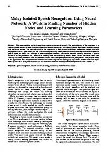
Human speech perception starts with receiving speech waveform through the ears. The speech will enter membrane basilar situated in the inner middle ear at which the signal waveform will be analysed and produced spectrum signal. The spectrum signal will enter neural transducer which converts the signal to neural activities at the ear’s nerve. The neural signal activities are translated into language code and the message will be sent to the brain for perception. Figure 1 shows the schematic diagram of the process.

Figure 1. Human perception model.

The speech recognition system model built in this paper imitates the human perception model. Three levels of processes are required for recognition by machine that are the acoustic processing, features extraction and recognition. The analogue speech will be sampled, digitised and filtered. These processes convert the signal into discrete form. The signal is then decided for the start and end points so that only the signal with information will be analysed. The next


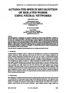
process is to extract features from the signal within the start and end points. This experiment used Linear Predictive Coding (LPC) for spectral analysis and speech features representation. The number of frames from the resulted features differs from one utterance to other. Therefore, frame normalization need to be applied to become equal to the number of input nodes in neural network used in this experiment. The data for testing and training will go through the same processes. The training data will be fed into neural network to optimise learning process which lies in updating iteratively the weights between networks layers. Upon having optimised weight, it will be used to test the training patterns. Figure 2 shows the processes involved in speech recognition using neural network.

coefficient representing features of the frame or known as features vectors. Speech is highly varies in term of its duration, acoustic information and resulted pattern even for a similar word utterance by same speaker at different time. Therefore, the number of frames per speech pattern will be most likely different from each other. Since number of input to the neural network is fixed, the number of speech pattern frame need to be normalized prior to feed into the network for training or testing. There are three possibilities of the number of frames after features extraction which are: a. Number of frame is equal to the number of input node. b. Number of frame is less than the number of input node. c. Number of frame is greater than the number of input node. Based on the possibilities the normalized algorithm is developed as in pseudo-code at Figure 4.

Speech Signal Pre-Emphasis s(n) = s(n) - 0.95s(n-1)

Figure 2. Speech recognition model using neural network.

3. Experimental Data This experiment uses digit utterances from four speakers consist of two males and two females in their 20’s. Each speaker uttered digit “0” up to “9” for 20 times. The utterances were recorded at different time to get utterance variation from speakers that is speakers may utter a same word differently at different time. They were told to speak clearly without any dialect or slang. The utterances were recorded using high quality microphone and sound editor software called GoldWave at a silence lab environment. Human speech puts much of its sound energy in the 200 Hz to 3.2 kHz frequency band [3]. Therefore, sampling size chosen for recording is 8 KHz which is twice the frequency of the original signal and follows the Nyquist rule of sampling. Human speaks continuous speech. However, the speech is considered static during short period of within10-50ms [7, 14]. Therefore, in this experiment every 20 ms, the speech will be analysed using spectrum analysis algorithm to extract the information representing the speech. As mentioned earlier, the work used LPC for spectral analysis as the speech parameters extracted using fix window of size 20ms and overlapped windows of size 10ms with number of order equal to 12. The LPC process can be described as in Figure 3. Each analysed frame will produce 12 LPC

Frame Blocking x(n)=s(Li+N)

Hamming Window W(n)=0.54-0.46cos(2πn/N)

Auto Correlation Analysis

R(m)=

N −1− m

∑ s(n)s(n + m)

m =0

LPC Computation s(n)≅ a1s(n-1)+a2s(n-2)+ ......aps(n-p)

Figure 3. Flow diagram of LPC processing.

Basically, the normalization scheme works by squeezing and expanding the features linearly. If the frame number is equal to the number of FIXFRAME that is the number of input node, then it will just copy as the features pattern for neural network training or testing. The second case is if the number of pattern frames is greater than FIXFRAME, then the pattern will be squeezed based on the ratio of the different. Similarly, if the number of pattern frames less than FIXFRAME, then the pattern will be expanded based on the ratio of the FIXFRAME and the pattern frames. This normalization is known as linear normalization.

Malay Isolated Speech Recognition Using Neural Network: A Work in Finding Number of Hidden…

1.

Read Signal X (0 … N) 2. If N == FIXSIZE, % case 1: equal size Xnew(n) = X(n); % copy 3. If N > FIXSIZE % case 2: bigger than Ratio = N/FIXSIZE; % calculate ratio Xnew(0 …FIXSIZE) = X(n* Ratio); 4. If N < FIXSIZE % case 3: smaller than Ratio = FIXSIZE /N % calculate ratio Xnew((0..FIXSIZE) = X(n*Ratio); FillEmpty (Xnew (i) = X(i+1));

5. Amplitude Normalization of signal X to 0 and 1

Figure 4. Normalization pseudo code.

The resulted pattern after normalization is as shown in Figure 5(a) and 5(b) for both cases of pattern size is greater and less than the fix features size respectively. Each pattern will pass through the processes described before fed into neural network for training and testing. All together, there are 800 patterns used in the experiment from which halves are for training and the remaining are for testing.

have one input layer, one hidden layer and one output layer. The features vectors representing speech pattern after the normalization is fed into neural network at input layer. These values are passed to the hidden layers and output layers through the connected weight between each layer. The output from each relation connection is calculated by summing the weight and the values between the connected layer and feed into non linear function like sigmoid and hyperbolic tangent functions. The calculation can be shown as follows. O u ti =

f ( n e ti ) =

 f  

∑

W ij O u t

j

j

 +θi  

(1)

Outi is the ith output value from the layer we want to calculate. Outj is the node jth output value from the preceding layer. Wij is the weight value connected between the calculated outputs layers ie. Outi and Outj. θ i is bias value at the calculated layer. The bias plays role in enhancing the learning process [11].

4.1. Training and Learning of the Network The neural network in this work is MLP supervised learning. The scheme for training is back propagation with sum square error. The sum square error calculated as follow N

E =

1 2

∑

j=1

a) Original size greater than fix features (2360:820).

(2)

(e j)2

where ej=(tj-oj) and N is the number of input, t is the desire target output and o is the output gotten from the network based on the square error. For example the desired output of the pattern representing a word “sembilan” is t[4] = {0.1, 0.0, 0.0, 0.1} while the output from the network is o[4] = {0.09, 0.05, 0.05, 0.09}. The sum square error for the first input pattern, j =1 can be calculated as below. e1 = [ ( t[0] - o[0] )2 + ( t[1] - o[1] )2 + ( t[2] - o[2] )2 + ( t[3] - o[3] )2 ] = 0.0001 + 0.0025 + 0.0025 + 0.0001 = 0.0052

b) Original size less than fix features (360:820).

Figure 5. Original size.

4. The Neural Network The neural network model used in the experiment is Feed Forward Multi Layer Perceptron (FFMLP). Reviews show that three layers MLP with one hidden layer can be a universal classifier [6]. An experimental result showed that the use of two hidden layers does not give better result compare to one hidden layer [12]. Therefore, this experiment use three layer MLP that

Each error of ej like the above example influences the total sum error from network the learning process. Therefore, if the error is big then the sum error is big implying the bad learning. The learning process in back propagation is done through minimizing the sum error through updating the weights using methods known as steepest descend which can be simplify as in the equation below. ∆w

ji

= ηδ

pj

O

pi

(3)


where η is the learning rate, δpj is the signal error at nod j from L layer and Opi is the output for node i from L-1 layer. The value of δpj is calculated as (4) δ p j = ( t p j − O p j ) O p j (1 − O p j )

output nodes value approaching 0.1 is consider “on” and the value near to 0.0 is consider “off”. The problem occurs is how do we determine the suitable threshold value as to which the value need to be grouped as “on” or “off”.

if it is the output node and δ

pj

= O

pj

(1 − O

pj

)∑ δ

pk

w

(5)

kj

k

if it is a hidden node. Based on equation 3, the value of learning rate, η determines the slope size of the equation that is how long the learning process take. The right choice of η is needed for a faster convergence. However, large value of η may lead to unstable learning. To help enhancing learning process, momentum rate, α is added to the equation 3 to become the following equation. ∆w

ji

( n + 1) = η (δ p j O

pi

) + α∆w

ji

(6)

(n )

The value of the momentum rate, α take into consideration the changes of the previous weight. The network training process can be illustrated as in Figures 6 and 7 show the flow diagram of back propagation scheme. Figure 7. Back propagation training scheme. Input features vectors of the pattern

Table 1. Target output nodes digit representation. Input Node

Update weight to minimize error

Digit 0 1 2 3 4 5 6 7 8 9

Hidden node

Output node

Error does not satisfy?

Figure 6. Training process.

4.2. Output Node Pattern Representation The network is a supervised network where target output is used to supervise learning process by error reduction. Therefore, the output nodes for the training pattern need to be well represented. The network model in this experiment use four nodes to represent speech pattern consist of digit “kosong” up to “sembilan”. These nodes will be classified as the speech by giving logic value “on” and “off” on each nodes in form of binary. Table 1 shows the target output representation for digit “0” to “9”. The value 0.0 indicates the node is “off” while 0.1 indicates the node is “on”. The values 0.0 and 0.1 are selected through trial and error. After training process, the values of output nodes will change depend on the network learning progress. An example for the output nodes after training can be shown as in Table 2. It can be observed in Table 2 that the outputs do not have exact value of 0.0 and 0.1 as in the target. However, after the training process the

O[0] 0.0 0.1 0.0 0.1 0.0 0.1 0.0 0.1 0.0 0.1

Output Nodes O[1] O[2] 0.0 0.0 0.0 0.0 0.1 0.0 0.1 0.0 0.0 0.1 0.0 0.1 0.1 0.1 0.1 0.1 0.0 0.0 0.0 0.0

O[3] 0.0 0.0 0.0 0.0 0.0 0.0 0.0 0.0 0.1 0.1

Table 2. An example of output nodes after training. Digit 0 1 2 3 4 5 6 7 8 9

O[0] 0.00012 0.10219 0.00023 0.12182 0.00012 0.08226 0.00010 0.08221 0.00003 0.07862

Output Nodes O[1] O[2] 0.00027 0.00006 0.00010 0.00020 0.04808 0.00091 0.06562 0.00022 0.00021 0.04763 0.00011 0.09762 0.09722 0.10021 0.05672 0.07562 0.00032 0.00031 0.00011 0.00043

O[3] 0.00008 0.00007 0.00061 0.00010 0.00071 0.00081 0.00022 0.00021 0.10110 0.67123

4.3. Speech Pattern Classification The classification was done by having two phases threshold comparison to decide whether a node is


grouped as “on’ or “off”. The two threshold values are 0.04 for the first phase and 0.006 for the second phase. The values are chosen by trial any error. The classification is done as in Figure 8. Each node will be compared with first threshold value 0.04. If the value is bigger than the threshold value then it will be labelled as “on”. The nodes that fail the first threshold are compared with the second threshold as not to miss selected. If the node is greater than the threshold, then it will also be labelled as “on”. The next step is to map the answer through binary representation

Figure 8. Classification method.

5. A Quest for Neural Network Learning Parameters and Number of Hidden Nodes There are factors that influence the network learning process. Some of them are the choice of learning parameters and network topology. As mentioned in section 4.1, the learning and momentum rate play important roles in enhancing network learning process. While suitable number of hidden node gives better mapping of the network input to output connection [11]. There are several experiments done to find the suitable learning and momentum rate. The best value however is not the same for all cases. This experiment used pairs of learning and momentum rate that have been used for speech recognition study using neural network [10]. In this experiment, five pairs of learning and momentum rate are chosen for the experimentation from which four pairs have been used previously on speech recognition by neural network experimentation. The pair {0.9, 1.0} is chosen randomly. The experimental learning and momentum rate pairs are shown below. Momentum Learning Rate

0.5 0.25

0.5 0.75

1.0 0.9

0.9 1.0

0.1 0.9

In finding suitable number of hidden nodes, some suggestions are given by previous researchers. Among the suggestions are, h = n, h = 2n, h = n, m [11] dan h = 3n [4] where n is the number of input nodes and m is the number of output nodes. Nevertheless, these suggestions are not suitable if the input node is large like in this experiment. Because it will lead to

biggest number of hidden nodes and thus lead to complexities and time consuming. Therefore, based on trial and error approach, this experiment chose number of hidden nodes start at 30 up to 70 with increment of 5 that is as in the set {30, 35, 40, .., 60, 65, 70}.

5.1. Experimental Set Up The purpose of this experimental is to find the suitable pairs of learning and momentum rate and number of hidden nodes for recognition of Malay isolated digit using neural network. This experiment is therefore divided into two phases that are to find the suitable pairs of learning rate and momentum rate and to find suitable number of hidden nodes. In the first phase that is to find the suitable pairs of learning and momentum rate, the controlled parameters which are the topology of neural network, number of epoch, error termination criterion, and initial weight are chosen as in Table 3. While in second phase experiment to find the suitable number of hidden nodes, the controlled parameters are set as in Table 4. Each parameter will go through training process. The training process will terminate either the error termination satisfied or the number of epoch satisfied. Table 3. Controlled parameters for finding pairs of learning and momentum rate. Error Termination Number of Epoch Network Topology Initial Weight Range

0.0001 6000 360:30:4 [-3:+3]

Table 4. Controlled parameters for finding the number of hidden nodes. Error Termination Number of Epoch Network Topology Initial Weight Range Learning Rate Momentum Rate

0.0001 6000 360: ? :4 [-3:+3] Result from previous Experiment

The training or the learning process is done with 320 input data from the speakers from which each digit is introduced 32 times to the neural network. These input data that is the order of digit “0” to “9” are fed into the neural network randomly as shown at Figure 9. The reason in randomly feed into the neural network is to help the neural network make better generalization of the pattern. The connection weights from each training session is saved and used in the testing.


pair has better error convergence from start error to end error. Table 5. experimental result on pairs of learning and momentum rate. Learning Rate (Eta)

Figure 9. Input digit pattern feed into neural network for training.

5.2. Testing Testing is done on different set of 320 speech patterns where each digit is tested 32 times. The testing set is a new set never introduced to the neural network. The test patterns were fed into neural network randomly just to make sure the neural network do not memorize the pattern but able to make generalization in recognition. The recognition rate is calculated by comparing number of true recognized pattern to the total number of tested patterns. Assuming X is the set of test pattern, n is the total number of test patterns and R(x) is the recognition function where 1 if true recognized R(Xi) = 0 if false recognized

0.25 0.5 1.0 0.9 0.1

Momentum Rate (Alpha) 0.5 0.7 0.9 1.0 0.9

Recognition Rate

Start Error

End Error

90% 92% 20% 92%

1.38584 0.96896 2.26425 2.405 1.3676

0.0003 0.0002 1.76007 2.405 0.0002

6.2. Number of Hidden Nodes The experimental result in finding the suitable number of hidden nodes is shown at Table 6. Figure 10 illustrate the result in graph recognition versus number of hidden nodes from 30 to 70. Table 6 shows that for all number of hidden nodes using the chosen learning parameters from the first experiment gives recognition rate of above 90%. At number of hidden nodes equal to 30, the recognition rate is 92%and increase to 93% at number of hidden nodes equal to 40. The maximum recognition rate of 95% was at number of hidden nodes equal to 45 and 50. The recognition starts to decrease to 93% again at number of hidden nodes equal to 55 up to 70.

Therefore, the recognition rate is calculated as n

recognition

rate

∑ =

R(X i)

i=1

n

x 100

Other than recognition rate, the neural network learning convergence is also taken into consideration to evaluate the best parameters. The learning can be shown in error graph versus iteration time for each training set.

6. Experimental Result 6.1. Learning Rate and Momentum The results of all set of test parameters are shown in Table 5. Table 5 shows that the pairs of learning and momentum rate {0.25, 0.5}, {0.5, 0.75} and {0.1, 0.9} achieved recognition rate above 90%. While the pairs of {1.0, 0.9) only get 20% recognition rate with very slow error convergence activity. The pair {0.9, 0.1} did not have any learning activities based on the learning graphic of no error reduction. The computer ‘hang’ when testing was made. All the testing parameter set terminate based on number of iteration criterion of 6000 epoch and do not reach error termination of 0.0001. It can be noticed that training set of pair {0.5, 0.75} and {0.1, 0.9} has the lowest end error of 0.00021. Nevertheless, for next experiment of finding the suitable number of hidden nodes, pair {0.5, 0.75} is used as the constant as the

Figure 10. Graph of recognition rate versus number of hidden nodes. Table 6. Experimental result on number of hidden nodes. Number of Hidden Nodes 30 35 40 45 50 55 60 65 70

Recognition Rate

Starting Error

Ending Error

92 % 92 % 93 % 95 % 95 % 93 % 93 % 93 % 93 %

0.96896 0.77195 0.84084 0.84922 0.81826 0.84016 1.27723 0.75126 1.07863

0.00021 0.00026 0.00093 0.00010 0.00029 0.00053 0.00547 0.00475 0.00086

7. Conclusions It can be concluded from the experiment that the learning parameter and number of hidden nodes


influence the ability of neural network classification. In finding the suitable learning and momentum rate, it is found that although the pair of learning and momentum rate that was used successfully by others on the same field may not give good result on different data. This can be observed through the learning and momentum rate pair of {1.0, 0.9} where the recognition rate was only 20% and the error convergence shows a very slow error decrement. The experiment also indicates that if the pairs of learning and momentum rate were chosen badly and wrong then the network can not learn at all. This can be shown at the pair {0.9, 1.0} where the error does not decrease at all and stay at constant value of 2.4050. The effect of number of hidden nodes can be seen at Figure 10 where the maximum recognition rate was only achieved at hidden nodes 45 and 50. Number of hidden nodes that is smaller than 45 would give lower recognition rate and if the number is greater than that 50 will also lead to lower recognition rate. In this experiment the best hidden nodes for this application is 45 due to it’s converge satisfy the error termination criterion of 0.0001 while the others did not.

[2]

[3]

[4]

[5]

[6]

8. Discussion and Enhancement

[7]

The parameters in this experiment are gotten from trial and error method. The result indicated that the method is reliable and could give good choices in finding the learning parameters and neural network topology. Nevertheless, the method does not try all possible solutions set of parameters. In our case, we selected only 5 pairs of momentum and learning rate and 9 choices of number of hidden nodes, whereas there maybe better solutions not selected for testing. The method also takes lengthy time prior to get result. For example, if one set of experimental solution takes 8 hours then 80 hours is needed to try 10 possible solution parameters sets. Whereas, the solution may not be within that choices and thus require more time to take. Therefore, for future enhancement, we suggest the use of automatic, robust and faster way in finding neural network learning parameters and topology through a method known as Genetic Algorithm (GA). Review shows that GA was able to find good neural network parameter set on other optimisation problem and pattern recognition faster [1, 2, and 5]. The works on automatic search for neural network parameters for speech problem by GA is an ongoing research and heading a good direction.

[8]

[9]

[10]

[11]

[12]

[13]

[14]

References [1]

Behzadian K., Kapelan Z., Savic D., and Ardeshir A., “Stochastic Sampling Design Using A MultiObjective Genetic Algorithm and Adaptive Neural Networks,” Computer Journal of

Environmental Modelling & Software, vol. 24, no. 4, pp. 530-541, 2009. Hyun K. and Kyung S., “A Hybrid Approach Based on Neural Networks and Genetic Algorithms for Detecting Temporal Patterns in Stock Markets,” Computer Journal of Applied Soft Computing, vol. 7, no. 2, pp. 569-576, 2007. Khalifa O., Khan S., Islam M., Mukhtar M., and Yaacob Z., “Speech Coding for Bluetooth with CVSD Algorithm,” in Proceedings of RF and Microwave Conference, Malaysia, pp. 227-229, 2004. Lippmann P., “An Introduction to Computing with Neural Network,” Computer Journal of IEEE ASSP Magazines, vol. 2, no. 3, pp. 4-22, 1988. Mohsen S., Morteza A., and Ali Y., “Design of Neural Networks Using Genetic Algorithm for the Permeability Estimation of the Reservoir,” Computer Journal of Petroleum Science and Engineering, vol. 59, no. 1, pp. 97-105, 2007. Pandya S. and Macy B., Pattern Recognition with Neural Network in C++, CRC Press, Florida, 1996. Parsons W., Voice and Speech Processing, McGraw-Hill, New York, 1987. Pierce R., “Whither Speech Recognition?,” Computer Journal of JASA, vol. 46, no. 4, pp. 1029 -1051, 1969. Rabiner L. and Juang H., Fundamental of Speech Recognition, Englewood Cliffs, Prentice Hall, 1993. Salam M., Muhammad D., and Salleh H., “Improved Statistical Speech Segmentation Using Connectionist Approach,” International Journal of Computer Science, Science Publication, vol. 5, no. 4, pp. 275-282, 2009. Sallehuddin R., Ngadimin M., Shamsuddin M., “Penentuan Saiz dan Bilangan Nod Tersembunyi Rangkaian Neural Bagi Peramalan,” Computer Journal of Teknologi Maklumat, FSKSM,UTM, vol. 5, no. 4, pp. 67-78, 1999. Salleh S., Mcinnesst R., and Jack A., “Enhanced Automatic Speaker Verification Based on Combination of Hidden Markov Models and Multi Layer Perceptron,” in Proceedings of MICC, Langkawi Malaysia, pp. 20-23, 1995. Turban E., Expert System and Artificial Intelligent, Republic of Singapore: Max Millan Publishing Company, 1999. Young S., “A Review of Large Vocabulary Continuous Speech,” Computer Journal of IEEE Signal Processing Magazine, vol. 13, no. 5, pp. 45-57, 1996.


Md Salam is a lecturer in the Faculty of Computer Science and Information System at Universiti Teknologi Malaysia (UTM). He holds Master degree from UTM and Bachelor degree from University of Pittsburgh USA in computer science. Currently, he is doing PhD in the field of speech recognition and artificial intelligent at UTM. Dzulkifli Mohamad is a senior lecturer and a professor in the Faculty of Computer Science and Information System at Universiti Teknologi Malaysia (UTM). He holds PhD and Master degree from UTM, post grad, Diploma from University of Glasgow, UK and Bachelor degree from Universiti Malaya, Malaysia. He has supervised many post graduate students in the fields of computer vision, image processing and artificial intelligent. His research interest include pattern recognition, digital image processing and artificial intelligent.

Sheikh Salleh is a senior lecturer and a professor in the Faculty of Biomedical Engineering and Health Science Universiti Teknologi Malaysia (UTM). He holds PhD degree from Edinburgh University, UK, Master degree from UTM and Bachelor degree from University of Bridgeport, USA. He has supervised many post graduate students in the field of biomedical engineering and speech processing. His research interest includes heart sound, infant hearing screening and speech processing.